Statistical Methods, Analyses and Applications for Next-Generation Sequencing Studies.

for Next-Generation Sequencing Studies

by Yan Yancy Lo

A dissertation submitted in partial fulfillment of the requirements for the degree of

Doctor of Philosophy (Biostatistics)

in the University of Michigan 2015

Doctoral Committee:

Associate Professor Sebastian K. Z¨ollner, Chair Professor Gon¸calo Abecasis

Professor Betsy Foxman Professor Timothy D. Johnson Assistant Professor Hyun Min Kang

To my husband, Henry, who is my source of support.

To my sister, Wai, who is my source of joy.

And to God,

who is the source of all wisdom.

The pursuit of my doctorate degree has been a rewarding yet extremely humbling experience. This dissertation would not have been possible without the support and guidance from my committee, colleagues, friends and family.

First, I would like to express my deepest gratitude to my committee chair, Dr. Sebastian Z¨ollner, who introduced me to statistical and population genetics when I was in transition between graduate programs. Since then, he has provided me invaluable research opportunities and guidance to build a solid foundation in genetics and biostatistics. He has been extremely patient, accommodating and encouraging. His excellent mentorship has helped me mature as an independent scientist and as an individual alike.

I would like to extend the gratitude to Dr. Gon¸calo Abecasis, who is always able to offer insightful advice for my research projects. I am also extremely grateful for the financial support Dr. Abecasis has provided for my graduate studies. I would also like to express my heartfelt thanks to Dr. Betsy Foxman, who has provided me valuable advice on the biological motivations of statistical methods, which has expanded my understanding of genetics and epidemiology. I truly look up to Dr. Foxman as my role model of a successful woman scientist. I would also like to thank Dr. Hyun Kang and Dr. Timothy Johnson for their patient instructions both inside the classrooms and specific to my research projects.

has offered tremendous help on my scientific writing. I have benefited greatly from her instruction on becoming a better writer. I would also like to thank the past and current members of the Z¨ollner lab, in particular Matthew Zawistowski, Ziqian Geng, Mark Reppell and Keng-han Lin, for their generous exchange of scientific ideas. The same gratitude goes to my colleagues at the Center for Statistical Genetics and the Department of Biostatistics, whom I have spent a lot of time learning, working and having fun with. I truly treasure our scholastic discussions and friendships.

Next, I would like to thank my friends from the Ann Arbor Chinese Christian Church who are more than friends - they are my family away from home. They have never ceased to express their support and care for me. My graduate studies in Ann Arbor have been genuinely blessed with many fond memories and lifelong companionships with these wonderful people.

Last but not least, I would like to thank my husband, Henry Fan, my parents, Norman Lo and Man-Yee Chan, and my sister, Wai Lo, for their continuous en-couragement and support. My family has shown me that love surpasses all physical distances and intellectual understanding; it is their unconditional love that has kept me motivated throughout the ten years of higher education in the United States.

DEDICATION . . . ii

ACKNOWLEDGEMENTS . . . iii

LIST OF FIGURES . . . vii

LIST OF TABLES . . . viii

ABSTRACT . . . ix

CHAPTER I. Introduction . . . 1

II. Comparing Variant Calling Algorithms for Target-Exon Sequencing in a Large Sample. . . 10

2.1 Introduction . . . 10

2.2 Methods . . . 13

2.2.1 Data description . . . 13

2.2.2 Variant calling . . . 14

2.2.3 Variant quality control . . . 16

2.3 Results . . . 19

2.3.1 Summary of variant call sets . . . 19

2.3.2 Overall quality of variant call sets . . . 20

2.3.3 Evaluating singleton variants . . . 21

2.3.4 Evaluating non-singleton variants . . . 24

2.3.5 Alternative implementations of variant callers . . . 26

2.3.6 Multi-allelic variants . . . 26

2.3.7 Computational burden . . . 27

2.4 Discussion . . . 28

2.5 Conclusions . . . 31

2.6 Appendix . . . 33

2.6.1 Pre-variant calling data processing . . . 33

2.6.2 Variant quality control . . . 33

2.6.3 Validation experiment . . . 37

2.6.4 Evaluation of singletons on additional dataset . . . 38

2.6.5 Supplementary figures and tables . . . 40

III. Markov Chain Monte Carlo Estimation of Sequencing Errors Using Over-lapping Reads . . . 45

3.1 Introduction . . . 45

3.2.2 Markov chain Monte Carlo algorithm for machine errors . . . 50

3.2.3 Model for estimating fragment errors . . . 51

3.2.4 Simulation . . . 52

3.2.5 Sequencing data analysis . . . 54

3.3 Results . . . 56

3.3.1 Simulation results . . . 56

3.3.2 Sequencing data results . . . 57

3.4 Discussion . . . 61

3.5 Appendix . . . 65

IV. RESCORE: Resolving Overlapping Reads Dependence in Next-Generation Sequencing Data . . . 68

4.1 Introduction . . . 68

4.2 Methods . . . 71

4.2.1 The RESCORE algorithm . . . 71

4.2.2 Evaluating RESCORE . . . 74

4.3 Results . . . 76

4.3.1 Recalibrated scores comparison . . . 76

4.3.2 Effect of bin size in RESCORE . . . 78

4.3.3 Variant calling comparison . . . 80

4.4 Discussion . . . 82

V. Whole-genome sequencing of uropathogenicEscherichia coli reveals long evolutionary history of diversity and virulence . . . 88

5.1 Introduction . . . 88 5.2 Methods . . . 90 5.2.1 Study design . . . 90 5.2.2 Variant calling . . . 91 5.2.3 Phylogenetic analyses . . . 93 5.3 Results . . . 95 5.3.1 Whole-genome phylogeny . . . 95

5.3.2 Phylogeny of virulence factors . . . 100

5.4 Discussion . . . 103

VI. Discussion. . . 109

BIBLIOGRAPHY. . . 115

Figure

2.1 Distribution of coverage at the individual carrying the singleton alternative allele . 22 2.2 Distribution of average coverage of sequence read data from 7,842 unrelated

Euro-pean individuals . . . 40 2.3 Average coverage at the 57 targeted genes in the AMD sequencing study . . . 41 2.4 Distribution of AMD singleton site coverage . . . 41 2.5 Proportion and average quality score of IBC singletons identified by PBC at

differ-ent sample sizes . . . 42 3.1 Two sets of machine error rates used in simulations, represented in PHRED scale . 54 3.2 Posterior mean error estimates from error sets 1 and 2 . . . 57 3.3 Marginal distribution of estimated machine errors by read cycle and quality score . 58 3.4 Read cycle and quality score components of machine errors estimated from the

MCMC algorithm . . . 59 3.5 Machine error (eM) estimates averaged across 10 samples . . . 60

3.6 Fragment error (eF) with respect to quality scores of pairs of overlapping bases,

averaged across 10 samples . . . 61 3.7 Likelihood convergence plot for simulated error rate set 1 . . . 65 3.8 Trace plots of representative parameters over the range of parameter space . . . 66 3.9 Potential scale reduction factor (PSRF) averaged across all parameters per sample 66 3.10 Marginal machine errors by (a) read cycle and (b) quality score . . . 67 4.1 Cartoon description of the RESCORE algorithm . . . 72 4.2 Insert size distribution of 40 samples from the BRIDGES Consortium . . . 75 4.3 Recalibrated quality scores from overlapping read pairs processed by RESCORE

versus soft-clipping methods . . . 78 4.4 Recalibrated quality scores against original base quality scores of the overlapping

bases, when the two original scores were equal . . . 79 4.5 Recalibrated quality scores of RESCORE for different bin sizes . . . 80 4.6 Venn diagram showing the number and Ts/Tv of >Q20 novel variants from each

dataset . . . 81 5.1 Phylogeny constructed from whole-genome assembly-based variants . . . 97 5.2 Unrooted trees derived from three selected virulence factors for uropathogenic and

commensal E. coli . . . 102 5.3 Classifications based on presence and absence of several virulence factors, described

in Marrs et al. [74], Tarchouna et al. [111] and Yun et al. [135], and multilocus sequence typing (MLST) . . . 107

Table

2.1 Summary statistics of 27,500 top-ranked SNPs per call set and quality assessed by

transition-to-transversion ratio (Ts/Tv) . . . 20

2.2 Heterozygous mismatch (a) between sequence calls and GWAS genotypes at 378 on-target GWAS markers, (b) between 80 sequence replicate pairs and (c) between pairs of algorithms . . . 24

2.3 Heterozygous mismatch (a) between each call set and GWAS genotypes at 378 on-target markers, and (b) between additional heterozygous genotypes in more complex algorithms and the GWAS markers . . . 26

2.4 Quality of call sets assessed by transition-to-transversion ratio (Ts/Tv), broken down by variant class and frequency . . . 43

2.5 Validation experiment results . . . 44

3.1 Samples analyzed by the proposed error rates model . . . 55

5.1 Summary table of pathotype classification scheme, adapted from Marrs et al. [74] . 91 5.2 Samples description of the pilot study . . . 92

5.3 Pairwise sequence differences of strains belonging to the same ST . . . 99

5.4 Summary of virulence gene trees . . . 101

5.5 List of virulence factors in each sampled strain . . . 108

Statistical Methods, Analyses and Applications for Next-Generation Sequencing Studies

by Yan Yancy Lo

Chair: Sebastian Z¨ollner

Current genetics studies rely heavily on next-generation sequencing (NGS) tech-niques. This dissertation addresses methodological developments and statistical strategies to efficiently and accurately analyze the large amounts of NGS data, thereby to understand the genetic contributions to diseases.

In chapter 2, we evaluated the benefits of different variant calling strategies by per-forming a comparative analysis of calling methods on large-scale exonic sequencing datasets. We found that individual-based analyses identified the most high quality singletons, but had lower genotype accuracy at common variants than population-based and LD-aware analyses. Therefore, we recommend population-population-based anal-yses for high quality variant calls with few missing genotypes, complemented by individual-based analyses to obtain the most singleton variants.

In chapters 3 and 4, we addressed the issue of overlapping read pairs in NGS studies arising from short fragments. In chapter 3, we proposed novel models to sep-arately estimate machine and fragment errors of a NGS experiment from overlapping

machine and fragment errors were largely predicted by the reported quality scores of the overlapping bases and were uniform across individual samples from the same experiment. In chapter 4, we proposed an algorithm, RESCORE, to resolve the fragment dependence while retaining machine error estimates in overlapping reads. When compared to soft-clipping the overlapping regions, RESCORE increased the recalibrated base quality scores for the majority of overlapping bases, leading to a decrease in estimated false positive rate of novel variant discovery.

In chapter 5, we presented an application of whole-genome sequencing for un-derstanding the evolutionary history of uropathogenicEscherichia coli (UPEC). We sequenced 14 UPEC and 5 commensals at >190x, and found a deep split between UPEC and commensal E. coli. We observed high between-strain diversity, which suggests multiple origins of pathogenicity. We detected no selective advantage of vir-ulence genes over other genomic regions. These results suggest that UPEC acquired uropathogenicity a long time ago and used it opportunistically to cause extraintesti-nal infections. In summary, this dissertation presented practical strategies for NGS studies that will contribute to further genetic advances.

Introduction

Since the publication of the first finished-grade human genome sequence in 2004 [36], scientific resources and efforts have been heavily allocated to develop genome analysis technologies [106]. In the past decade, particularly the past few years, genome analysis has shifted from using first-generation capillary sequencing to next-generation sequencing [5, 71]. Next-next-generation sequencing (NGS) is the massively parallel, high-throughput technology that allows the generation of large amounts of genetic data [72, 77]. In contrast to capillary sequencing technologies, which typically produces 500-800 bases per reaction and required over three years and three million dollars to sequence one human genome [36, 92], NGS platforms are able to generate in a much shorter time and lower cost large numbers of short reads that can be reconstructed into the full genome [7, 107]. The recent Illumina HiSeq X Ten is the first platform to deliver full coverage human genomes for close to a thousand dollars, with the yield of up to 6 terabases per day, which is approximately 2000 times of the number of bases in a full human genome [34, 119].

Rapid advancement in sequencing technologies has prompted the success of nu-merous genetics studies, with a common goal of cataloging variations among human populations or populations of other species [41, 44, 93, 102, 113, 116]. An

rate and detailed database of genetic variations has extensive biological and medical applications. For example, the 1000 Genomes Project sequenced the genomes of

>2,500 individuals from populations around the world and created a detailed cata-log of human genetic variations, including variants with population allele frequency as low as 1% [116, 117]. This catalog of variation complemented many sequencing and genome-wide association studies in improving data quality and expanding sam-ple sizes, thereby increasing the power to detect associations between genetic loci and complex diseases [51, 110, 121].

As large-scale sequencing studies become more widespread, the analyses of indi-vidual genomes have led to discoveries of novel rare polymorphisms (allele frequency

<1%), which were difficult to detect from small samples or from genotyping chips which identify alleles from predetermined genomic positions [120]. Rare polymor-phisms are of particular interest and importance, because they are more likely to be functional [12, 69, 95]. In the recent study published by Nelson et al. [82] that sequenced over 14,000 individuals at 202 drug targeted genes, they discovered rare variants as frequent as one every 17 base pairs; over half are expected to be delete-rious. Moreover, rare polymorphisms have shown to have larger effects on disease phenotype than common polymorphisms [1, 15, 21]. Therefore, identifying such rare variants can explain significant proportions of the missing heritability [48, 139]. From the population genetics perspective, variants are rare because they arise from the re-cent past. NGS analysis of over 6,500 exomes suggested that most protein-coding variants are rare and have recent origin of 5000-10000 years [24]. The excess of rare variants present in the current population indicate that the human population has expanded faster than exponentially in the recent past [43, 99].

statistical methods are required to further the understanding of the contributions of genetic variation to complex traits. Indeed, the studies mentioned above were successful due to the development of a large range of statistical methods and analysis pipelines designed for NGS studies [17, 40, 54, 61]. However, to date there is no single pipeline that works uniformly the best in all NGS studies; the quality and quantity of variant discovery depends heavily on the statistical methods and bioinformatics tools used [90, 133]. While the curation of variants is very important to minimize false discoveries, the optimal variant discovery strategy should also minimize false negatives in order to make the best use of the data. Moreover, errors generated along the multiple steps of a sequencing experiment can accumulate and be misinterpreted as rare variants. In fact, NGS techniques are believed to have relatively higher error rates than chip genotyping or capillary sequencing techniques [94, 98, 107]; therefore the older technologies are still frequently used to validate selected variants from NGS studies [65, 82, 136].

In this dissertation, we proposed novel statistical methods and analysis plans to address the challenges in NGS data. We considered different variant calling al-gorithms for obtaining the most complete set of variants in large-scale sequencing datasets. We devised a strategy for estimating separate sources of sequencing errors in an NGS experiment. We proposed and implemented a method to correct for the dependence in overlapping pairs of sequence reads. Finally, we designed and carried out a whole-genome deep-sequencing study to understand the evolutionary trajecto-ries of virulence genes in pathogens. The dissertation concludes with a discussion of the implications and significance of our methods for the development of NGS studies. In the sections below, we provide a more detailed overview of each chapter.

Variant calling in large-scale NGS studies

Variant discovery, or variant calling, plays a central role between raw NGS data and applications. Capillary sequencing directly reads the alleles at each position, and genotyping chips start with a set of known variant sites and type each individual sample’s alleles at these sites; in contrast, NGS determines the alleles at each genomic position statistically based on the combined evidence from the short reads spanning the position [58, 59, 76, 86]. Therefore, variant calling typically improves with high coverage, because of the increased information at each position.

Sequencing experiments targeted at exonic regions or specific genes are popular because these regions potentially harbor most functional variants or variants of inter-est [6]. At a fixed cost, sequencing only these genomic regions allows the expansion of sample size. By examining a lot of individuals, these sequencing studies of exonic regions aim to identify rare variants contributing to complex traits [6, 67, 115]. With high coverage and large sample size, these studies tend to apply simple variant call-ing algorithms, which typically call genotypes from the reads covercall-ing each position per individual (individual-based caller) [58, 59]. However, coverage is often hetero-geneous due to the uneven capturing of the targeting technology [68, 77]. Therefore, sites with insufficient coverage may benefit from sophisticated calling algorithms used in low-coverage sequencing studies, which call genotypes based on population allele frequency (population-based caller) [17, 40, 49] or based on genotypes in linkage disequilibrium (LD) in the sample (LD-aware caller) [61, 70].

In chapter 2, we evaluated the potential benefits of different calling strategies by performing a comparative analysis of variant calling methods on exonic data from multiple large-scale sequencing datasets [82, 136]. We call variants using

individual-based, population-based and LD-aware methods with stringent quality control. We measure genotype accuracy by the concordance with on-target GWAS genotypes and between 80 pairs of sequencing replicates. We validate selected singleton variants using capillary sequencing.

Using these strategies, we found that individual-based analyses identified the most high quality singletons. However, individual-based analyses generated more missing genotypes than population-based and LD-aware analyses. Individual-based genotypes were the least concordant with array-based genotypes and replicates. Population-based genotypes were less concordant than genotypes from LD-aware analyses with extended haplotypes. Therefore, we recommend population-based analyses for high quality variant calls with few missing genotypes. With extended haplotypes, LD-aware methods generate the most accurate and complete genotypes. Finally, individual-based analyses should complement the above methods to obtain the most singleton variants.

Segregating sources of sequencing error in NGS reads

Variant calling in NGS studies are often complicated by sequencing artefacts and errors; such artefacts and errors typically lead to low-quality variant calls [86, 91]. Rare variant discovery requires particular care because sequencing errors are often mistaken as rare variants [12, 52, 55]. Methods have been developed to detect and filter variant calls that are likely false positives [20, 40]. An additional set of methods have been developed to remove the effect of sequencing artefacts from the reads [40, 76, 91] and to adjust for known errors [53] prior to variant calling. Despite these efforts, not all error sources in a sequencing experiment are known and accounted for [100]. In particular, variant calling relies on the base quality score of each sequenced

base, but the score reported by the sequencing machine typically reflects multiple sources of errors, and requires recalibration to reflect the empirical error rates [76]. To properly adjust for these errors, we need to understand and disentangle error sources in an NGS experiment.

In chapter 3, we proposed a statistical model for estimating two common sources of error in an NGS experiment, namely machine error which arises from the sequencing machine and fragment error which occurs in the DNA fragment prior to base-calling. These two errors can be separately estimated from overlapping read pairs, arising from short fragments. Overlapping read pairs replicate any errors in the underly-ing fragment sequenced. However each read in the pair is an independently read by the sequencing machine, hence generating two estimates of the machine errors. We proposed models for machine errors and fragment errors based on concordance and discordance of overlapping bases, using base quality scores and read cycles as predictors. We designed a Markov chain Monte Carlo algorithm to sample from the posterior distribution of the errors, and analyzed 10 samples with over half of the reads overlapping.

We found that machine errors were mainly predicted by reported base quality scores, while they were mostly constant across read cycles, with only a slight increase in error rates at the last few cycles. These error rates were uniform across samples from different plates and lanes, suggesting that machine errors are consistent within a sequencing experiment. As for fragment errors, they were also uniform across samples. However, we found that fragment errors were predicted by the base quality scores of concordant overlapping bases, as opposed to the previous assumption that fragment error rates are uniform across the genome [20]. Therefore, our models demonstrated the utility of overlapping reads for better understanding the error

sources in sequencing experiments.

Resolving overlapping reads in NGS data

Overlapping read pairs are common sequencing artefacts in many NGS studies. Since these read pairs replicate fragment error at the overlapping regions, overlapping reads need to be treated before variant calling; falsely assuming independence would lead to overestimation of genotype calling accuracy, inflating the number of singleton variants. To address this problem, some studies have soft-clipped (discarded) one of the overlapping reads in each pair. This solves the dependence problem, but is an overcorrection because each read still contain independent machine errors. In chapter 4, we proposed an algorithm, RESCORE, to retain the combined machine information from both reads while removing the fragment dependence. We repre-sented the combined machine error estimate from a pair of overlapping bases as a temporary quality score, and utilized base quality score recalibration to map the temporary scores to reflect the empirical mismatch rate at each position.

We then applied RESCORE to analyze 40 samples from a whole-genome sequenc-ing study with 8x coverage, where each sample had over half of its reads overlappsequenc-ing. RESCORE increased the recalibrated base quality scores for the majority of overlap-ping bases when compared to soft-clipoverlap-ping the overlapoverlap-ping regions. This increment led to an almost 20-fold decrease in the estimated false positive rate of novel variants, which would result in the discovery of 0.027% additional variants that were likely to be genuine. Therefore we recommend incorporating RESCORE as a standard data processing step in NGS analysis pipelines.

Whole-genome sequencing of uropathogens

Genetic variation among pathogenic bacterial strains can be informative of the evolution and diversity of infectious disease phenotypes [8, 66, 102]. In Chapter 5, we presented an application of whole-genome sequencing for understanding the evo-lutionary history of uropathogenic Escherichia coli (E. coli). Uropathogenic E. coli (UPEC) are phenotypically and genotypically very diverse. This diversity makes it challenging to understand the evolution of UPEC adaptations responsible for causing urinary tract infections (UTI). To gain insight into the relationship between evolu-tionary divergence and adaptive paths to uropathogenicity, we sequenced at deep coverage (190x) the genomes of 19 E. coli strains from urinary tract infection pa-tients from the same geographic area. Our sample consisted of 14 UPEC isolates and 5 non-UTI-causing (commensal) rectal E. coli isolates.

We developed a novel pipeline for the phylogenetic analysis of the E. coli strains. We identified strain variants usingde novo assembly-based methods. Based on pair-wise sequence differences across the whole genome, we clustered the strains using a neighbor-joining algorithm. We examined evolutionary signals on the whole-genome phylogeny and contrasted these signals with those found on gene trees constructed based on specific uropathogenic virulence factors.

The whole-genome phylogeny showed the divergence between UPEC and com-mensal E. coli strains without known UPEC virulence factors happened over 32 million generations ago, which is equivalent to 107,000- 320,000 years [88]. Pairwise diversity between any two strains was also high, suggesting multiple genetic origins of uropathogenic strains in a small geographic region. Contrasting the whole-genome phylogeny with three gene trees constructed from common uropathogenic virulence

factors, we detected no selective advantage of these virulence genes over other ge-nomic regions. These results suggest that UPEC acquired uropathogenicity a long time ago and used it opportunistically to cause extraintestinal infections.

Conclusion

Next-generation sequencing technologies are rapidly advancing, as are statistical analysis and methodology developments, in order to efficiently and accurately pro-cess the high-throughput data. This dissertation develops methods in the upstream processing of NGS data and provides an application of NGS analysis for under-standing the evolution of bacterial virulence. These studies together provide novel directions and promising perspectives for analyzing NGS datasets, thereby improving the confidence in the interpretation of NGS data.

Comparing Variant Calling Algorithms for Target-Exon

Sequencing in a Large Sample

2.1 Introduction

With rapid advances in sequencing technology, large-scale sequencing studies en-able discovery of rare polymorphisms. Exome and targeted sequencing studies are especially popular in the studies of complex traits. These designs focus on small genome regions likely to be enriched for functional variants [6, 67, 115], achieving higher coverage of an important subset of the genome and facilitating larger sample sizes [41, 68]. While variant calling typically improves with increasing read coverage [7], exome and targeted experiments tend to generate uneven coverage. For studies averaging 40x to 120x, empirical coverage per targeted position per sample can range from less than 5x to over 150x [11, 75, 84, 136]. At high coverage, genotypes can be called with high precision using basic calling strategies [6]. However, at regions with local low coverage, calling genotypes accurately is challenging, leading to more errors and missing data [17]. In studies with low mean coverage, advanced variant calling algorithms compensate by combining read information with linkage disequilibrium (LD) information across large samples [61, 125]. However, it is unclear if such al-gorithms substantially improve genotypes in datasets with heterogeneous coverage.

This chapter is published as Lo, Y. et al. 2015. BMC Bioinformatics, 16(1), 75.

To address this question, we evaluated the performance of advanced variant calling algorithms in targeted sequencing experiments. Our goal was to provide specific guidelines for applying variant calling algorithms to these studies.

Variant calling algorithms fall into three major categories depending on how infor-mation from shotgun sequencing data is aggregated across individuals and genomic positions [86]. The first category involves individual-based single marker callers (IBC), which assign genotypes based on aligned reads from a single individual at a single position [28, 58, 59, 60, 76]. These callers are typically applied to high-depth exome sequencing data [11, 84]. The second category of algorithms is population-based single marker callers (PBC), where reads per position from all samples jointly determine polymorphism and allele frequencies. Based on estimated allele frequen-cies, these methods then call genotypes using per individual read data [17, 49]. PBC is typically used in low-pass sequencing studies [61, 116, 117]. The third category of calling algorithms utilizes linkage disequilibrium (LD) information across several hundred kilobases flanking each variant base identified by an IBC or PBC [61, 70]. Similar to widely used imputation algorithms [9], these LD-aware calling methods (LDC) phase existing variant calls into haplotypes, then update genotypes accord-ing to the joint evidence across similar haplotypes. LDC, though computationally demanding, have been used in combination with PBC to successfully interpret low-coverage, genome-wide data such as that in the 1000 Genomes Project [116, 117].

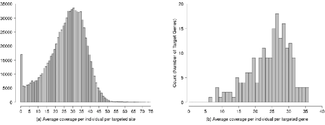
To compare the performance of the three types of algorithms in large-scale se-quencing datasets with high coverage, we analyzed 7,842 European individuals, each sequenced at 202 targeted genes [82]. The average per targeted site per individual coverage was 24x, but with a wide range from 0 to > 75x (Figure 2.2). Genotype data from previous genome-wide association studies (GWAS) provided long

haplo-types for LD-aware genotype calling. We generated four sets of variant calls from this dataset, using (1) IBC, (2) PBC, (3) LDC based on only the sequencing data and (4) LDC after combining the sequencing data with flanking GWAS data. We focused on a fixed number of variants per call set after ranking the variants by quality control metrics, and assessed the quality of each filtered call set by transition to transversion ratio and the percentage of called variants confirmed in SNP databases. Moreover, we evaluated genotype accuracy by collating 80 pairs of experimental replicates and by comparing sequencing calls with on-target genotypes from previous GWASs. We further validated a subset of caller-specific singletons at the heterozygous individuals with an independent capillary sequencing experiment. Finally, to ensure applicabil-ity of our comparison findings to other studies, we investigated our dataset using alternative approaches of IBC and PBC. We also generated IBC variant calls from an additional dataset with average coverage of 127.5x, sequenced at 57 genes from 3,142 individuals [136], and compared these calls with their existing PBC call set.

We found that at a fixed number of variant sites, IBC identified a larger propor-tion of extremely rare variants of high quality, particularly singletons, while capturing most of the common polymorphic sites that were identified by the other callers. We replicated the result in the additional high-coverage dataset and by using different variant caller implementations. However, IBC genotypes at common variants were of the lowest quality by all measures. They were the least concordant with GWAS genotypes and within sequencing replicate pairs. Moreover, the IBC call set con-tained 4.72% missing genotypes, due to low coverage or low quality calls. In the PBC set, the percentage of missing genotypes dropped to 0.47% by using a popu-lation allele frequency prior. PBC also showed improved heterozygous concordance with on-target GWAS genotypes as well as between replicates. Without flanking

markers, LDC achieved similar genotype accuracy with PBC, while further reducing the missing genotypes to 0.17%. With extended haplotypes from flanking GWAS markers, LDC achieved the same level of missing genotypes (0.17%) and the highest genotype concordance among all callers.

2.2 Methods

2.2.1 Data description

To understand the strengths and limitations of individual-based, population-based and LD-aware variant calling methods, we analyzed sequence read data from 7,842 unrelated European individuals. The next-generation sequencing data was part of a large-scale targeted sequencing experiment generated for the purpose of identifying variants associated with 12 common diseases and cardiovascular and metabolic phe-notypes, previously described in Nelson et al. [82]. This experiment targeted 2,218 exons of 202 genes of potential drug interest, covering 864kb (≈ 1%) of the coding genome. Each exon was captured to include the coding sequence plus UTR and 50 bp flanking sequence on each end. Each sample had on average 0.6 million 100 bp paired-end Illumina reads, with overall average depth of 24x, but depth averaged per individual per targeted site ranged from 0x to over 75x (Figure 2.2a). In particular, six genes had low mean coverage (<10x) across all exons; the mean coverage across gene regions and across individuals spanned a range of 7x to 35x (Figure 2.2b).

Among the 7,842 individuals considered, 80 were independently sequenced twice. All 7,842 individuals had been previously typed on one of Illumina (300k, 550k, 610k) or Affymetrix (500k, 6.0) chips for genome-wide association studies (GWASs). Prior to variant calling, we aligned reads using BWA 0.5.9 (http://bio-bwa.sourceforge. net) [56] with human genome build 36 as reference. We removed duplicate reads using Picard (http://picard.sourceforge.net/). We recalibrated base quality

scores using Genome Analysis Toolkit (1.0.5974) from the Broad Institute [76]. We combined the GWAS genotype data from various chips using PLINK [97] (See Section 2.6).

2.2.2 Variant calling

We used likelihood-based models for genotype and SNP calling, as outlined in Li et al. [61]. For each of the 10 possible genotypes (AA, AC, AT, AG, CC, CT, CG, TT, TG, GG) at each locus, the model computes genotype likelihoodP r(reads|genotype). These likelihoods are calculated per genomic position with aligned reads. Base qual-ity scores of the reads are refined using the base alignment qualqual-ity (BAQ) adjustment to account for base calling error rates and mapping uncertainty [53]. Using Bayes’ rule, these likelihoods are combined with a model-specific prior on the genotype

π(genotype) to generate posterior probabilities P r(genotype|reads). We considered 3 categories of calling algorithms that reflect how information is aggregated across individuals and positions.

Individual-based single marker caller (IBC)

IBC applies an individual based prior which assumes each allele has a probabil-ity θ = 0.001 of being different from the reference. For variant sites, we assigned uniform prior probabilities for transitions and transversions to avoid bias in the evaluation based on transition to transversion ratio (Ts/Tv). By computing the genotype likelihoods using aligned reads per individual, the model assigns the most likely genotype when the posterior probability reaches a threshold of 99%; geno-types with lower posterior probability are marked as missing. We used glfSingle (http://genome.sph.umich.edu/wiki/GlfSingle) to call genotypes. By calling also the reference homozygous genotypes, we obtained the union set of all variant

sites and genotypes across all individuals.

Population-based single marker caller (PBC)

PBC uses a two-step procedure to call variants [61]. First, upon observing at least one read carrying a non-reference allele, the model applies a population genetic prior that estimates the probability of the site being polymorphic as a function of sample size, with per base pair heterozygosity of θ = 0.001 under the stationary neutral model [126]. As with IBC, the model assumes a prior with uniform Ts/Tv. Second, per polymorphic site, PBC estimates the population allele frequency f us-ing aligned reads from all individuals, assumus-ing a biallelic site in Hardy-Weinberg equilibrium. These allele frequency priors combine with the likelihoods calculated per individual to generate posterior genotype probabilities. We used the PBC im-plemented as glfMultiples (http://genome.sph.umich.edu/wiki/GlfMultiples), which also generated variant calls for NHLBI GO Exome Sequencing Project (ESP) and contributed to 1000 Genomes Project analyses [114, 116, 117].

In this study, we used a posterior probability threshold of 99% for the most likely genotype, which was the same threshold as for the ESP [114]. To maintain indepen-dence between experimental replicates, we generated two call sets, each including 7,762 unique samples plus 80 samples, one from each sequence replicate pair.

LD-aware caller (LDC)

Starting from a set of variant calls, LDC updates the genotype of each individual at each marker using a Hidden Markov Model derived from the haplotype-based model used in the imputation software MACH [62]. The LDC algorithm starts with randomly phased haplotypes for each individual. Per iteration, the algorithm compares one sequenced sample with a randomly picked subset of haplotypes. It

updates each genotype or imputes missing genotypes, based on the similarity of the sample haplotype to the reference haplotypes. In addition to identifying the most likely genotype, LDC calculates the expected number of reference alleles carried by each individual (dosage). Per variant site, LDC also estimates the correlation coefficient R2 between true allele counts and estimated allele counts, as a measure of imputation quality. This caller, previously used in low-pass sequencing studies [61, 116], has been implemented as ThunderVCF (http://genome.sph.umich.edu/ wiki/ThunderVCF).

We used LDC to refine each of the two PBC call sets described above. We applied the standard setting of 30 iterations and 200 reference haplotypes per iteration. We considered two scenarios with different haplotype information: First, we applied LDC on short haplotypes, which consisted only of the PBC variant calls at the sequences captured in the sequencing experiment. Second, we created long haplotypes by combining PBC variant calls with GWAS-genotypes from flanking markers within 500 kb from both ends of each target gene. In both scenarios, we masked GWAS genotypes within the target regions and used these markers as measures of genotype quality.

2.2.3 Variant quality control

To remove potentially false variant calls caused by technical artifacts, we followed the filtering and support vector machine (SVM) approach used in the ESP [114] and Zhan et al. [136]. Initial filtering included quality metrics based on read alignments, nearby indels and excess heterozygosity (See Section 2.6.2). For LD-aware calls, we imposed an additionalR2 _{quality control criterion, which filters sites withR}2 _<0.7.

SVM generates a summary score for each site based on the initial quality metrics, classifying good and bad calls with respect to training call sets (See Section 2.6.2).

We ranked these scores and selected the 27,500 top-ranked variants per call set for comparison. We set the cutoff to compare only variants with positive SVM scores.

After selecting 27,500 top-ranked variants per call set from SVM classification, we filtered individual genotypes to discard those with more than 1% estimated error. From IBC genotypes, we removed and marked as missing the genotypes with PHRED quality score less than 20 or with genotype depth less than 7x. As the quality of PBC genotypes is less affected by individual genotype depth, we only filtered with PHRED quality<20. Analogously, we filtered LD-aware genotypes with a posterior probability ratio < 99 : 1 between the genotypes with the highest and the second highest posterior probability. Comparing call sets

We compared 4 sets of 27,500 variants, generated using IBC, PBC, LDC with-out flanking haplotypes and LDC with flanking haplotypes. First, we evaluated the overall quality of each call set by calculating transition to transversion ratios (Ts/Tv), stratified by variant type as annotated by ANNOVAR (hg19, gencodeV7,

http://www.openbioinformatics.org/annovar/) [123] and by minor allele count. Second, we compared our call sets to the Single Nucleotide Polymorphism database (dbSNP, release 135,http://www.ncbi.nlm.nih.gov/SNP/), a recent public archive of confirmed variants.

We then characterized IBC-specific variants and PBC-specific variants by their Ts/Tv and read coverage. Most of the IBC- and PBC-specific variants were sin-gletons. We performed an independent capillary sequencing experiment on 32 IBC-specific and 41 PBC-IBC-specific singleton variants, sampled from individuals from the CoLaus study [82] carrying the singleton heterozygous genotypes (See Section 2.6.3). Error rates from this validation provided estimates of false discovery rates of caller-specific singletons. Finally, we extended the validation to 51 caller-caller-specific singletons

with SVM scores below the cutoff, to assess the quality of discarded sites from each set.

We assessed genotype quality of each call set by four summary statistics: (1) The percentage of missing genotypes from no calls and filtered genotypes (2) The pairwise heterozygote mismatch rates (he) between our genotype calls from sequencing and the genotypes from GWAS chips at the on-target markers. he is defined as the number of genotypes called as heterozygous in one set but homozygous in the other, divided by the total number of heterozygous genotypes in both sets. (3) he for the 80 sequence replicate pairs, at variant sites where at least one individual per pair is heterozygous. (4) The shared variants between each pair of call sets and calculated the he between every pair of callers.

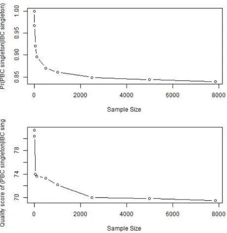
To investigate the effect of sample size on the difference in performance between IBC and PBC, we performed down-sampling analyses on our original dataset, eval-uating the ability of the PBC caller to identify variants called as singletons by IBC. For simplicity, we focused on variants that were called as singletons in the full dataset of 7,842 individuals (IBC singletons). We generated random samples of 50, 100, 500, 1,000, 2,500 and 5,000 individuals from the original dataset by sequentially adding individuals and used PBC to call variants in each of the samples. For each down-sampled dataset, we calculated the proportion of IBC singletons identified by PBC and recorded the genotype quality of these PBC singletons. We repeated the full random sampling experiment 10 times and averaged the results.

To assess if our results were driven by the specific choice of calling algorithms, we applied the individual- and population-based settings of GATK UnifiedGenotyper (version 3.1.1-g07a4bf8) [17] to our original dataset. The UnifiedGenotyper follows the same genotype likelihood framework described above for variant calling. In

par-ticular, it uses the same model for individual- and population-based calling, where it estimates simultaneously the population allele frequency and most likely geno-types. To generate individual-based calls, population size is set to 1. We generated individual- and population-based variants for our targeted exon data with 7,842 sam-ples. We compared the two resulting call sets, focusing on the singletons specific to each analysis.

To replicate our results in a second dataset with higher sequencing coverage, we considered an additional dataset obtained from the AMD Consortium, which se-quenced 3,142 individuals at 57 genes from 10 age-related macular degeneration loci [136]. The average coverage was 127.5x, but 10% of the genes suffered from low aver-age coveraver-age of around 10x (See Section 2.6.4, Figure 2.3). We generated IBC variant calls and compared them with existing PBC variant calls of this dataset, obtained from the project investigators. We evaluated the IBC-specific singletons, particularly those at sites with local low coverage, and contrasted them with singletons identified by IBC and PBC.

2.3 Results

2.3.1 Summary of variant call sets

In the complete call sets of 7,842 individuals, the individual-based single marker caller (IBC) generated 31,970 variants while the population-based single marker caller (PBC) generated 29,147 variants. The LD-aware caller (LDC) modified genotypes from PBC, hence it generated the same number of variants. We filtered each call set separately and ranked the variants using a support vector machine (SVM). We observed 30,297 IBC, 27,690 PBC variants and 27,535 LDC variants with positive SVM scores. To compare call sets for a fixed call rate, we focused on the top 27,500 variant sites from each set. In the IBC set, 59.4% of the calls were singletons (MAF

All SNPs Singletons

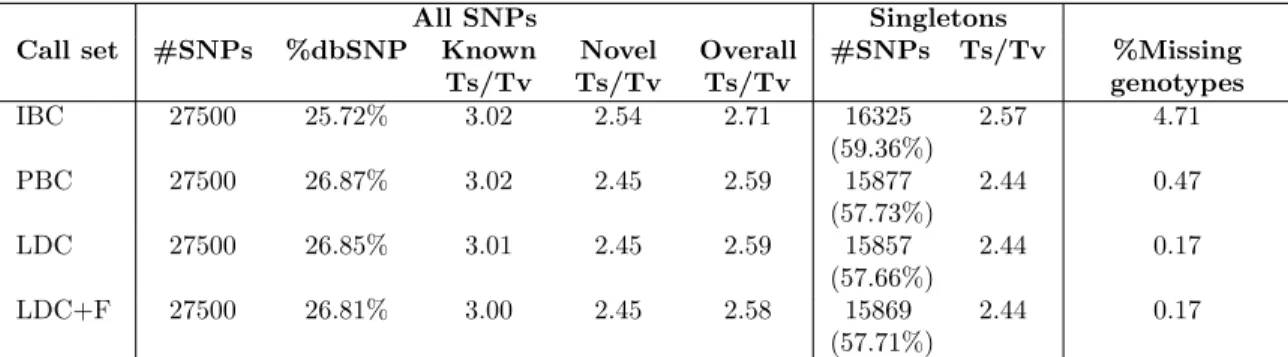
Call set #SNPs %dbSNP Known

Ts/Tv Novel Ts/Tv Overall Ts/Tv #SNPs Ts/Tv %Missing genotypes IBC 27500 25.72% 3.02 2.54 2.71 16325 (59.36%) 2.57 4.71 PBC 27500 26.87% 3.02 2.45 2.59 15877 (57.73%) 2.44 0.47 LDC 27500 26.85% 3.01 2.45 2.59 15857 (57.66%) 2.44 0.17 LDC+F 27500 26.81% 3.00 2.45 2.58 15869 (57.71%) 2.44 0.17

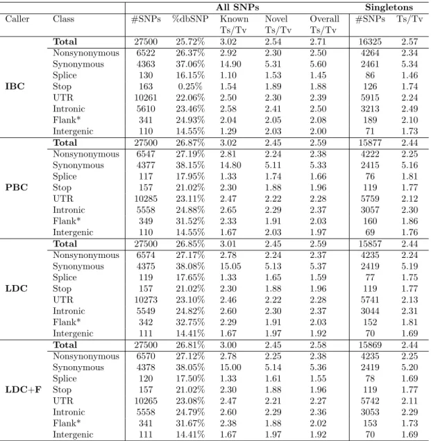
Table 2.1: Summary statistics of 27,500 top-ranked SNPs per call set and quality assessed by transition-to-transversion ratio (Ts/Tv). Abbreviations: IBC = individual-based single marker caller, PBC = population-based single marker caller, LDC = LD-aware caller without flanking haplotypes, LDC + F = LD-aware caller with flanking haplotypes. Expanded table showing quality of call sets broken down by variant class is included in Section 2.6 Table 2.4.

= 0.06%), while 57.7% of the PBC and LDC calls were singletons (Table 2.1). Over 81% of variants in each call set had minor allele counts ≤ 5. Most of these rare variants were novel; only 26-27% of variants from each call set were recorded in the dbSNP database (Table 2.1).

Combining our four filtered call sets each of 27,500 SNPs, our analyses generated a total of 29,652 autosomal SNPs. We identified 1,035 variants not previously found in the Nelson et al. analyses of the same dataset [82]. Among these, 509 (48.16%) were IBC-specific, while 445 (42.10%) were in all call sets. The IBC call set had the highest percentage of missing genotypes (4.72%), while the PBC call set had a substantially lower percentage (0.47%) (Table 2.1). The LDC call set had the lowest percentage of missing genotypes (0.17%). Typically LDC genotypes have no missing data; in our analysis, missing genotypes in LDC were a result of filtering genotypes with more than 1% uncertainty.

2.3.2 Overall quality of variant call sets

We assessed the quality of the variants included in the four call sets by calculating the transition-to-transversion ratio (Ts/Tv). A Ts/Tv>2 is expected for intergenic sites; Ts/Tv is typically much higher in coding regions due to purifying selection

[114]. In our data, Ts/Tv of the unfiltered IBC call set was 2.27, and Ts/Tv of the unfiltered PBC and LDC call sets were both 2.46. Ts/Tv of all call sets increased after SVM classification at the 27,500 variant cutoff (Table 2.1), indicating reasonable quality control. We then focused on the quality of these SVM top-ranked call sets. As Table 1 shows, the IBC call set attained the highest Ts/Tv of 2.71, while PBC and LDC without flanking haplotypes had a Ts/Tv of 2.59. LDC with flanking haplotypes had a Ts/Tv of 2.58.

Comparing Ts/Tv between known variants and novel variants, we observed that known variants (in dbSNP) generally had higher Ts/Tv than novel variants (Table 2.1). Singletons had slightly lower Ts/Tv compared to the corresponding overall call set, as singletons represent recent mutations that are less affected by purifying selec-tion [105]. Analogously, known variants had a higher Ts/Tv because such variants are typically older and have been subjected to purifying selection for longer.

At exonic variants, all call sets attained Ts/Tv greater than 3, with nonsyn-onymous variants having lower Ts/Tv than synnonsyn-onymous variants (Table 2.4). The coding variants had higher Ts/Tv than non-coding variants in all call sets, because coding sequences contains higher proportion of CpG sites enriched for transitions compared to non-coding regions, and because transitions are enriched at degenerate sites within coding regions. Intergenic and flanking variants had Ts/Tv around 2 in all call sets, consistent with expectations (Table 2.4).

2.3.3 Evaluating singleton variants

Most caller-specific variants were singletons. We found 4,203 caller-specific vari-ants out of 29,652 in the union call set. Of these, 1,850 (44.02%) were IBC-specific, 1,787 (96.59%) being singletons with Ts/Tv 1.97. On the other hand, 1,731 (41.18%) variants were shared between PBC and LDC sets, but not found by IBC. We

consid-Coverage=7x 0 10 20 30 40 50 60 70 80 90 100 110 120 130 140 150 0 100 200 300 400 500 600 Singleton Coverage Count

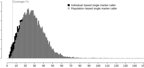
Individual−based single marker caller Population−based single marker caller

Figure 2.1: Distribution of coverage at the individual carrying the singleton alternative allele. We compare the distribution of coverage at called singleton variants between individual-based caller (black) and population-based caller (light gray). The overlap of the two distributions is in dark gray. Here we show all singleton variants after SNP filtering and genotype filtering on quality<20. We keep individual-based single marker calls at low genotype coverage for this comparison, with the vertical dash line indicating genotype coverage filter at 7x.

ered sites in this category as PBC-specific since LDC did not introduce new sites, but only modified genotypes at sites called by PBC. Of these PBC-specific sites, 1,260 (72.79%) were singletons with Ts/Tv 1.08.

IBC identified more singletons at low coverage than PBC, even after an additional filtering of all genotypes with less than 7x coverage (Figure 2.1). Independent capil-lary sequencing experiment validated 30 out of 30 (100%) IBC-specific singletons, and 38 out of 41 (92.68%) PBC-specific singletons (Table 2.5). This difference in valida-tion rates was not statistically significant (Fishers exact p-value = 0.258). Relaxing the SVM threshold to 29,000 SNPs per call set, IBC-specific and PBC-specific sin-gletons still had comparable validation rates, at 91.30% (42/46) and 92.45% (49/53) respectively.

Notably, 99.13% of PBC-specific sites were in the IBC unfiltered (complete) call set of 31,970, including all 471 sites with minor allele count>1. On the other hand,

only 177 (9.57%) IBC-specific sites were in the PBC complete call set of 29,147; the majority was undiscoverable using PBC. Therefore, we extended the validation experiment to IBC-specific singleton calls ranked below 29,000, where no singletons from PBC could be sampled from the CoLaus subset. Capillary sequencing showed that these IBC-specific singletons at the lowest ranks had a validation rate of 81.82% (18/22; Table 2.5).

To compare the performance of singleton calling between IBC and PBC in a differ-ent dataset with higher average coverage, we repeated these analyses on a targeted sequencing dataset of 3,142 individuals sequenced at a mean coverage of 127.5x [136]. We generated an IBC call set which contained 33,615 variants with Ts/Tv 2.12, while the existing PBC call set contained 31,527 variants with Ts/Tv 2.10. Comparing these two call sets, IBC called 1,913 more singletons than PBC. These additional singletons had Ts/Tv 1.63. Interestingly, the additional singletons with high quality were located in regions with low coverage. At depth <10x and with an extra genotype quality filter of > 10, IBC identified 864 additional singletons with Ts/Tv 2.18. At the same genotype depth and quality thresholds, IBC and PBC shared 911 singleton variant calls with Ts/Tv 2.13 (Figure 2.4). When we relaxed the genotype depth threshold to < 20x, IBC identified 1,360 additional singletons with Ts/Tv 1.90, while IBC and PBC shared 2,745 singletons with Ts/Tv 2.07.

We evaluated the impact of sample size on the difference in performance between IBC and PBC by down-sampling the data to sample sizes of 1, 50, 100, 500, 1,000, 2,500 and 5,000 and calling variants in these smaller datasets using PBC. We com-pared the PBC singletons from each down-sampled set to high-quality IBC singletons from the original dataset of sample size 7,842. We observed that for sample sizes>1, PBC failed to identify all IBC singletons. The proportion of IBC singletons called by

Heterozygous mismatch rate

IBC PBC LDC LDC+F

(a) All samples at 378 GWAS markers 0.82% 0.38% 0.39% 0.32% (b) 80 sequence replicate pairs at all called variants 1.01% 0.34% 0.36% 0.20% (c) Pairwise comparison of callers

vs PBC 0.42% – – –

vs LDC 0.93% 0.35% – –

vs LDC+F 1.01% 0.41% 0.30% –

Table 2.2: Heterozygous mismatch (a) between sequence calls and GWAS genotypes at 378 on-target GWAS markers, (b) between 80 sequence replicate pairs and (c) between pairs of algorithms.

PBC decreased as sample size increased. The quality score of the singletons called by PBC also decreased with sample size. At sample size = 100, PBC called 89.6% of the IBC singletons with average quality score of 73.7; at sample size = 5,000, the percentage dropped to 84.0% with average singleton quality score 69.5 (Figure 2.5).

2.3.4 Evaluating non-singleton variants

We assessed genotype quality of common variants by comparing genotypes at 378 on-target variants shared between all call sets and the GWAS data from the same individuals (Table 2.2a). The IBC call set had the highest discordance with GWAS genotypes, with heterozygous mismatch he = 0.82% discordant genotypes. While heterozygous mismatch rates were comparable between PBC and LDC with no flanking haplotypes, at he= 0.38% and 0.39% respectively, the rate was lower for LDC with flanking haplotypes, at 0.32% (Table 2.2a).

Genotype concordance between sequencing replicate pairs provided a second met-ric of robustness of each calling algorithm (Table 2.2b). he at replicate pairs followed the same qualitative trend as the GWAS comparison (Table 2.2a), where IBC had the highest he = 1.01% at replicate pairs. The heterozygous mismatch rates were 0.34% for PBC and 0.36% for LDC without flanking haplotypes. With flanking haplotypes, he = 0.20% between experimental replicates of LDC. This mismatch rate was lower than the he with GWAS genotypes, suggesting that the error rate of

chip-based genotyping was higher than the error rate for LDC genotypes.

The non-missing genotypes between each pair of call sets had less than 1% het-erozygote discordance (Table 2.2c). IBC and PBC call sets had low discordance, with he = 0.42%. The PBC and LDC call sets also had similar discordance, with

he = 0.35% and 0.41% respectively. The two LDC call sets were the least discordant, with he= 0.30%. IBC and LDC call sets had higher heterozygous discordance, with

he = 0.93% between IBC and LDC without flanking haplotypes, andhe = 1.01% be-tween IBC and LDC with flanking haplotypes. These mismatch rates were consistent with the above comparisons with GWAS genotypes and between sequence replicates (Table 2.2).

Complex calling algorithms called additional genotypes at sites that had missing calls at less complex calling algorithms (Table 2.3a). To evaluate specifically the quality of these additional sites, we calculated the heterozygous mismatch rates with GWAS genotypes (Table 2.3b). Comparing each algorithm with progressively more complex alternatives at the 378 on-target variant sites with GWAS information, we observe that the PBC call set contained 15,727 (5.68%) more heterozygous genotypes than the IBC call set, withhe= 0.85%. Thus PBC generates high-quality genotypes at most sites that cannot be called with IBC. LDC without flanking haplotypes generated 3,113 (1.06%) while LDC with flanking markers generated 3,664 (1.25%) more heterozygous genotypes than PBC. Mismatch rates in these extra genotypes varied widely between the two settings; calls from LDC without flanking markers had a mismatch rate of 2.41% while calls from LDC with flanking markers had an error rate of 0.71% (Table 2.3b).

All samples at 378 GWAS markers IBC PBC LDC LDC+F

(a) Number of heterozygous

genotypes (hets)

276,761 293,730 298,220 298,531

Heterozygous mismatch 0.82% 0.38% 0.39% 0.32%

(b) Number of additional

hets and heterozygous

mismatch

not in IBC 15,727 (0.85%) 17,937 (1.23%) 18,308 (0.47%)

not in PBC 3,113 (2.41%) 3,664 (0.71%)

not in LDC 1,145 (0.87%)

Table 2.3: Heterozygous mismatch (a) between each call set and GWAS genotypes at 378 on-target markers, and (b) between additional heterozygous genotypes in more complex algorithms and the GWAS markers.

2.3.5 Alternative implementations of variant callers

To evaluate the consistency of these observations across other implementations of variant callers, we analyzed the same dataset using GATK UnifiedGenotyper. We generated individual-based (G-IBC) and population-based (G-PBC) call sets. The G-IBC call set contained 34,704 variants with Ts/Tv 2.21, while the G-PBC call set contained 33,696 variants with Ts/Tv 2.23. Each call set contained about 32% singletons: the G-IBC call set contained 11,001 singletons with Ts/Tv 2.13, and the G-PBC call set contained 10,678 singletons with Ts/Tv 1.77. The proportion of singletons was substantially higher in our IBC call set (59.36%) generated using glfSingle and PBC call set (57.73%) generated using glfMultiples, as well as in pre-vious analyses of the same dataset (60.32%) [82] using the SOAP caller [59]. Since a high proportion of singletons identified by glfSingle and glfMultiples have been experimentally replicated or validated (see above), GATK UnifiedGenotyper is con-servative when calling singletons. Nevertheless, G-IBC identified about 3% more singletons than G-PBC and these had significantly higher Ts/Tv, replicating the pattern observed in our analyses using glfSingle and glfMultiples.

2.3.6 Multi-allelic variants

IBC identified 523 on-target SNPs with more than one non-reference allele. Of these, 513 SNPs (1.87% of 27,500 IBC SNPs) had two non-reference alleles (triallelic)

and 10 had three non-reference alleles. Following the population genetics calculations used in Nelson et al. [82], we predicted that∼0.9% of variants would be triallelic and that a third allele would be called at 0.5% of biallelic sites due to sequencing error. Under a model of homogeneous mutation rate, we would thus expect a proportion of ∼1.4% observed triallelic SNPs. Similar to others [30, 82], we observed an excess of triallelic SNPs.

Most of the triallelic variants were rare: 205 (38.53%) had two singleton non-reference alleles, and 253 (47.56%) had one singleton non-non-reference allele and one more common non-reference allele. For the 10 SNPs showing all four alleles, 8 had at least one singleton non-reference allele. Nelson et al. [82] validated 10 out of 10 singleton triallelic variants from the same dataset. Among the 523 multi-allelic variants called by IBC, PBC called 509 biallelic, identifying the non-reference allele with more information (higher allele frequency or higher read depth). PBC identified the remaining 14 multi-allelic SNPs as monomorphic.

2.3.7 Computational burden

The computational burden of variant calling increases when the algorithm ag-gregates more information across individuals and sites. Hence IBC is the fastest algorithm and LDC is the slowest. IBC used about 250 CPU-hours to generate all variants for all 7,842 individuals, while PBC used 400 CPU-hours. For IBC, each individual at a specific genomic region can be analyzed in parallel. For PBC, all individuals have to be considered jointly, but genomic positions are independent and can be analyzed in parallel. In terms of memory usage, IBC consumed negligible memory since it only needed to read in the genotype likelihoods for one position per individual. For PBC, memory consumption increased roughly linearly with sample size. To analyze our dataset with 7,842 individuals, the maximum memory usage was

7.9 Gb. In our down-sampling analyzes, sample sizes of 1,000 and 5,000 consumed 1.1 Gb and 5.3 Gb memory respectively.

The LDC model considers all haplotypes jointly, with run time increasing in quadratic scale with the number of haplotypes included in the reference panel, which is the state space of the underlying Hidden Markov Model. Other factors affecting run time included length of each haplotype, number of iterations, and total sample size. We performed LD-aware calling per gene for 15,684 haplotypes at 202 genes, using a reference panel size of 200 for 30 iterations. After running PBC, LDC with flanking haplotypes took about 3000 CPU-hours. Without flanking haplotypes, LDC took about 2000 CPU-hours. To speed up the process while retaining sufficient LD information, LDC can be run in parallel on larger genomic regions, such as a 1Mb re-gion or a chromosome. Memory usage increased linearly with the number of variants in the gene: each gene contained 300 to 2,000 variant sites after adding GWAS flank-ing genotypes, with the memory required for runnflank-ing LD-aware algorithm rangflank-ing from 45 Mb to 300 Mb.

We performed all analyses on a Dell C6100 blade server with four discrete dual 6-core Intel Xeon X5660 CPUs at 2.80 GHz. 128 GB RAM and 1 TB of local SATA disk were available on this system.

2.4 Discussion

We performed an extensive comparison between calling algorithms of various com-plexity on a large sequencing dataset capturing exons of 202 drug-targeted genes with mean coverage of 24x. As a result of the capturing process necessary for targeted sequencing, we observed a wide range of coverage per targeted position, echoing the outcomes of other exome sequencing studies aiming at high coverage [83, 136]. Thus,

our work provides general guidelines for using variant calling algorithms on exome and targeted sequencing datasets.

Existing calling algorithms aggregate different levels of information from sequence reads. We considered three major groups of likelihood-based models: (1) Individual-based single marker caller (IBC) uses aligned reads at each marker per individual, (2) population-based single marker caller (PBC) uses aligned reads at each marker for all samples to estimate population allele frequency, (3) LD-aware genotype re-finement caller (LDC) uses linkage disequilibrium information from loci surrounding each called variant. Many different approaches exist for each model; each uses a variation of individual-based, population-based or haplotype-based priors. Previous studies have shown comparable performance between glfSingle/glfMultiples and ear-lier versions of the GATK UnifiedGenotyper [64]. By comparing sets of IBC and PBC from the same developer, we observed excess high-quality singletons in individual-over population-based algorithms.

Comparing filtered call sets of identical size (27,500) for each caller, IBC discov-ered more rare variants than PBC. In particular, at lower coverage, IBC was able to identify more high-quality singletons than PBC. We replicated this result twice, in a second dataset with higher coverage and in the original dataset using a different approach of the callers. We observed that the ability of PBC to detect singletons depended on sample size: With increasing sample size, PBC identified fewer single-tons, and the quality of the identified singletons decreased. This advantage of IBC over PBC can be partly explained by the fact that in larger samples, singletons have an allele frequency <0.001. Hence the prior for a site being a singleton is stronger in the individual-based caller and less evidence is required to call a singleton.

call sets had>99% concordance at the high-quality, non-missing heterozygous geno-types. Our validation experiment confirmed all selected IBC-specific singletons, with very few unconfirmed singletons in the PBC call set. Moreover, most PBC-specific singletons were in the IBC unfiltered (complete) call set. We observed the same trend of IBC generating an augmented set of singletons in high coverage sequencing data (>120x), where IBC almost doubled the number of high-quality singletons at sites with local low coverage (<10x).

Furthermore, only IBC was capable of identifying polymorphisms with more than one non-reference allele, which led to discovery of an additional 1.9% of rare alleles in the sample. The excess of triallelic sites over the theoretical prediction of 1.4% is likely the result of heterogeneity of mutation rate due to sequence context and genomic environment. Existing associations between multiallelic variants and disease phenotypes [16, 31] suggest that properly accounting for such variants can increase the power of a sequencing study.

While IBC had strengths in identifying singletons, PBC generated better overall genotype quality. At common variants, PBC genotypes overcame low coverage at specific samples, achieving fewer missing genotypes and higher accuracy than IBC calls. The discordance between IBC and GWAS genotypes was low (0.82%), but more than two times higher than the GWAS discordant rates of the other call sets.

LDC achieves even higher genotype accuracy than IBC and PBC by using hap-lotype information to impute missing genotypes from an existing single-marker call set. Imputation is typically more effective with longer haplotypes. In our study, we created long haplotypes by combining sequencing data with SNPs from previous GWAS genotyping chips. LDC with such flanking haplotypes achieved the highest accuracy and the least missing genotypes. As targeted sequencing studies might not

have chip data to generate long haplotypes, we studied if LDC would still improve genotype accuracy with haplotypes based only on the sequencing data. Without flanking haplotypes, LDC had fewer missing data at the common variants over PBC, yet with a slightly higher mismatch rate. In particular, the additional heterozygote genotypes at common GWAS markers had a high mismatch rate of 2.43%, despite an overall mismatch rate of 0.39%. This suggested that using LDC on short haplotypes to impute missing genotypes created a relatively large number of imputation errors. Comparison between sequence replicates further demonstrated that LDC without flanking haplotypes had minimal benefit over PBC. As LDC imposes a considerable computational burden, it seems questionable whether this caller should be used when flanking haplotypes are not available.

2.5 Conclusions

In summary, while IBC generated high quality unique singletons, as well as mul-tiallelic variants, its resulting call set contained more missing genotypes and geno-typing errors at common variants. PBC calls showed a substantial decrease in the number of missing genotypes and errors over IBC calls at these variants. Only when flanking haplotypes were available, LDC calls showed noticeable refinement of PBC genotypes, resulting in a call set with the highest concordance with GWAS geno-types and between experimental replicates. Therefore, IBC had strengths in calling extremely rare variants, while PBC combined with LDC had strengths in calling the more common variants.

Based on these results, we recommend a two-fold calling strategy for targeted sequencing studies with medium to high coverage in a large sample. We recommend first to use a population-based single marker caller to generate accurate common

variants and most of the rare variants. Second, we recommend using individual-based single marker caller to enrich the call sets with additional singletons. If flanking markers around targeted regions are available, despite the computation burden, we recommend using LD-aware caller to refine and impute population-based calls at high accuracy, resulting in a complete call set.

2.6 Appendix

2.6.1 Pre-variant calling data processing Sequence read data

We aligned reads using BWA 0.5.9 (http://bio-bwa.sourceforge.net) with human genome build 36 as reference. Average mapping rate was 99.7%; 98.5% of reads were properly paired. Using Picard (http://picard.sourceforge.net/) we identified and removed 21% duplicate reads. We recalibrated the base quality scores using GenomeAnalysisTK-1.0.5974 (http://www.broadinstitute.org/gsa/wiki/ index.php/Base_quality_score_recalibration)[17].

Genotype data

We combined genotype data from previous GWASs typed on Illumina 300k, 550k, 610k and Affymetrix 500k and 6.0 using PLINK [97]. We identified 378 GWAS variants on the targeted regions. At these variants, we confirmed reference allele for A/T and G/C variants using sequencing calls and respective allele frequencies, and there were no strand flip issues. We discarded a small number of genotypes at the flanking regions based on ambiguous strand information.

2.6.2 Variant quality control Initial filtering

We applied to each call set initial filters, which were based on read alignments at variant sites and summary statistics of each site. In particular, at each polymor-phic site, we computed several Z-score test statistics of read alignments, including strand bias, allele balance and alternative allele inflation, with the detailed statistical tests described below. A SNP with extremeZ-scores indicate bias from mapping or sequencing artefacts which likely lead to false positive calls. Cutoffs for each filter

followed from the ones used in the NHLBI GO Exome Sequencing Project [114]. We further imposed an indel filter, which filtered SNPs located within 5 base pairs of known insertions or deletions from 1000 Genomes low-coverage CEU data (July 2010 release). We detected sites with excess heterozygosity than expected under Hardy-Weinberg equilibrium, calculated using inbreeding coefficient, described below. For LD-aware calls, we imposed an additionalR2 quality control criterion by filtering the sites with estimated squared correlation less than 0.7 between true allele counts and estimated allele counts. Here we describe in detail the filters used:

1. Strand bias: Conditioned on the site being biallelic, strand bias refers to higher than expected frequency of observing the alternate allele on the forward or the reverse strand. Specifically, the strand bias filter counts the number of reference and alternate alleles on each strand as a 2-by-2 contingency table. Under the null hypothesis, a genuine polymorphism should have the alternate allele observed equally often from forward and reverse strands. Therefore, the strand bias filter discards sites with normalized Z-score greater than 10 or absolute correlation greater than 0.15, which suggest strong association between strand and the allele observed.

2. Allele balance: Allele balance measures the ratio between allele counts from genotype calls and estimated allele counts calculated from individual sequence depth and likelihoods (http://genome.sph.umich.edu/wiki/Genotype_Likel ihood_Based_Allele_Balance). A small ratio indicates bias towards certain alleles at a called polymorphic site, which is likely to be false positives. We im-posed a lower bound of 67% on the allele balance ratio for good quality SNPs.