Multivariate Functional Regression and Selection

(1)

Multivariate Functional Regression and Selection

by Joseph Naiman

A dissertation submitted in partial fulfillment of the requirements for the degree of

Doctor of Philosophy (Biostatistics)

in The University of Michigan 2020

Doctoral Committee:

Professor Peter Song, Chair

Assistant Professor Walter Dempsey Assistant Professor Peisong Han Professor Kerby Shedden

(2)

Joseph Naiman [email protected] ORCID id: 0000-0002-9027-7569

c

(3)

This thesis is dedicated to my wife, Jessica, who has stood by me throughout the PhD program with love and support, and to my children, Dovi, Shira, Sari, Talya

(4)

ACKNOWLEDGEMENTS

First and foremost I would like to thank God for providing me with the insight, strength and guidance to complete this dissertation.

I am grateful to the Department of Biostatistics for providing me with the essential tools to complete this dissertation. The outstanding faculty and diversity in research helped guide me throughout my PhD studies.

My deepest gratitude goes out to my advisor, Professor Peter Song, who patiently guided me through my thesis work. Professor Song always made himself available despite his busy schedule and the multiple PhD students he is currently mentoring. Many thanks to the members of Song Lab who provided me with the data used in this dissertation. I am grateful for the insightful weekly discussions presented at Song Lab, and feel fortunate to have been part of the innovation and growth that happens there on a regular basis.

Thank you to my other committee members- Professor Walter Dempsey, Professor Peisong Han, and Professor Kerby Shedden- for their many contributions. Their feedback of my proposal helped shape the direction of my thesis, and for that I am grateful.

Thank you Professor Shedden and Professor Brenda Gillespie for allowing me to work at the Consulting for Statistics and Analytics Research (CSCAR) through-out the duration of my PhD program. At CSCAR I learned invaluable skills abthrough-out applying statistics to real life studies being conducted both within and outside the University. At weekly CSCAR meetings we tackled difficult statistical problems and

(5)

became better statisticians through the collaborative efforts of the staff and graduate students.

My endless gratitude to the many family members who helped make this disser-tation possible. I thank my parents, Mr. Amiel and Dr. Channah Naiman for their support. My mother has provided me with the motivation to pursue a PhD by serv-ing as a role model of teachserv-ing excellence, and her invaluable advice and guidance has helped me throughout the program. My in-laws, Dr. Ephraim and Mrs. Rose Zinberg, I thank for their ongoing support and availability to help with the kids. My father-in-law Mr. Jared Cohen, I thank for providing me with a job that allowed our family to manage financially as I pursued this PhD over many years and for being a role model of professional success.

As a father of four when I started this program, I was able to complete it only with the support of my wife and children. To my wife, Jessica, I thank for lovingly and patiently standing by me throughout the program. I am extremely grateful for the help of my wife and my mother in editing this dissertation.

(6)

LIST OF FIGURES

Figure

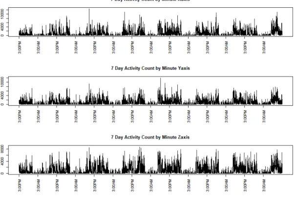
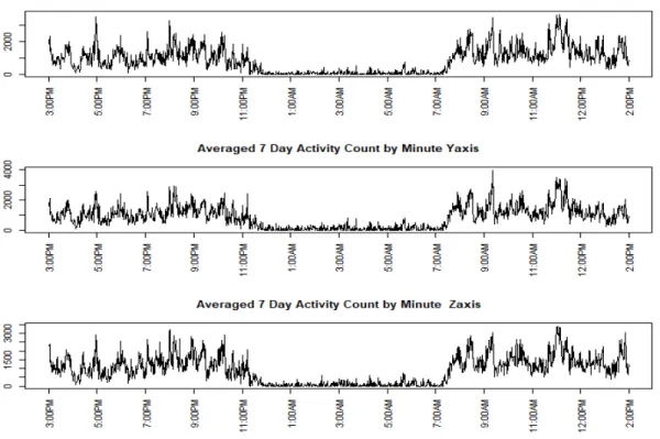
2.1 Estimated marginal functions with 95 percent shaded confidence bands of the function h evaluated at 100 grid points for each component while holding all other components equal to 0.5 in Scenario 2 . . . . 35 3.1 TriAxis Activity Count for the 7 Days of accelerometer wear . . . . 40 3.2 VM Activity Count for the 7 Days of accelerometer wear . . . 41 3.3 TriAxis Activity Count averaged minute-by-minute for the 7 Days of

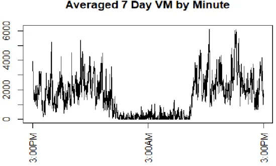
accelerometer wear . . . 41 3.4 VM Activity Count averaged minute-by-minute for the 7 Days of

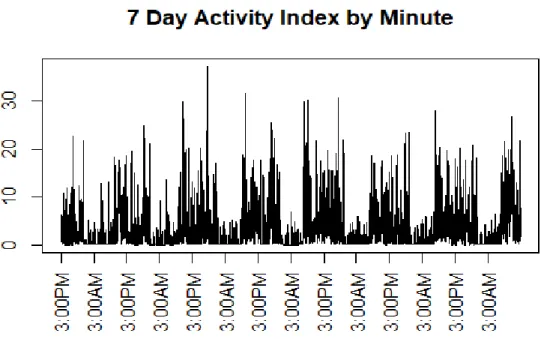
accelerometer wear . . . 42 3.5 AI for the 7 Days of accelerometer wear . . . 43 3.6 AI averaged minute-by-minute for the 7 Days of accelerometer wear 44 3.7 . . . 60 B.1 Leading Eigenfunction extracted for Tri-axis 7-day functional data . 106 B.2 Leading Eigenfunction extracted for VM 7-day functional data . . . 107 B.3 Leading Eigenfunction extracted for Tri-axis 1-day averaged

func-tional data . . . 107 B.4 Leading Eigenfunction extracted for VM 1-day averaged functional

data . . . 108 C.1 Leading Eigenfunction extracted from X(t) process for Tri-axis data 109

(10)

C.2 Leading Eigenfunction extracted from U(t) process for Tri-axis data 110 C.3 Leading Eigenfunction extracted from X(t) and U(t) process for VM 110 C.4 Leading Eigenfunction extracted from X(t) and U(t) process for AI 111

(11)

LIST OF TABLES

Table

2.1 Goodness of Fit for Scenario 1 . . . 29 2.2 Model Size for Scenario 1 . . . 30 2.3 FPC Selection for Scenario 1 . . . 30 2.4 Goodness of Fit via the concordance regression for Scenario 2 . . . . 33 2.5 Sensitivity and Specificity of Functional Selection for Scenario 2 . . 33 2.6 FPC Selection for Scenario 2 Functional Z1 _{. . . .} ₃₄ 2.7 FPC Selection for Scenario 2 Functional Z2 _{. . . .} ₃₄ 3.1 #FPC Scores that explain ≥50% . . . 55 3.2 FPCA Functional selection of 3-D Activity Count for X,Y and Z axis

for the 7 day functional . . . 55 3.3 FPCA Functional selection of 3-D Activity Count for X,Y and Z axis

for the 1 day averaged functional . . . 55 3.4 R2

AQ using the 7-day functional of 3-D Activity Count . . . 56

3.5 R_AQ2 using the 7-day functional of VM Activity Count . . . 56 3.6 R_AQ2 using the 7-day functional of AI . . . 56 3.7 R2

AQ using 1-day averaged functional of 3-D Activity Count . . . . 56

3.8 R2

(12)

3.9 R_AQ2 using 1-day averaged functional of AI . . . 57

3.10 R2 AQ for Simulated acceleromter data Scenarios 1 and 2 . . . 62

3.11 Sensitivity and Specificity of Functional Selection . . . 62

3.12 Feature Selection for Scenario 1 . . . 63

3.13 FPC Selection for Scenario 2 . . . 63

4.1 SFPCA R2_AQ using the 7-day functional of 3-D Activity Count . . . 72

4.2 SFPCA R2_AQ using the 7-day functional of VM Activity Count . . . 73

4.3 SFPCA R2 AQ using the 7-day functional of AI . . . 73

4.4 #FPC Scores that explain ≥50% . . . 73

4.5 % of variance explained from the decomposition Z(t) =X(t) +U(t) 73 4.6 SFPCA Functional selection of 3-D Activity Count for X,Y and Z axis 74 4.7 SFPCA R2_AQ using the 7-day functional of 3-D Activity Count using X(t) and U(t) process. . . 75

4.8 SFPCA R2 AQ using the 7-day functional of VM Activity Count. . . . 75

4.9 SFPCA R2 AQ using the 7-day functional of AI using U(t) and X(t), 76 4.10 SFPCA Functional selection of 3-D Activity Count for X,Y and Z axis for U(t) process. . . 76

(13)

LIST OF APPENDICES

Appendix

A. Proofs and additional Tables from Chapters 2 . . . 95 B. Additional Graphs for Chapters 3 . . . 106 C. Additional Graphs for Chapters 4 . . . 109

(14)

ABSTRACT

With the pervasiveness of sensor data, real-time physiological signals and behav-ioral data are often collected in many biomedical studies. This thesis is motivated by data collected from a tri-axis accelerometer ActiGraph GT3X, a device that measures acceleration in the 3-D directions with a sampling frequency of 30-100 Hz. The cen-tral task is to relate this multivariate functional quantity with various scalar health outcomes of interest in the presence of other scalar covariates.

In the first project, we propose a new methodological framework of semi-parametric regression models that allow the study of a non-linear relationship between a scalar response and multiple functional predictors in the presence of scalar covariates. The proposed methodology is termed as MFRS (Multivariate Functional Regression and Selection). Utilizing functional principal components analysis (FPCA) and least-squares kernel machine methods (LSKM), we substantially extend the classical semi-parametric regression model of scalar responses on scalar predictors, in which multiple functional predictors are included in the non-linear model. Regularization is estab-lished for feature selection in the setting of reproducing kernel Hilbert spaces. The proposed method enables us to perform simultaneous model fitting and variable selec-tion on funcselec-tional features. For implementaselec-tion, we propose an effective algorithm to solve related optimization problems, in that iterations take place between both linear mixed models and a variable selection procedure (e.g. sparse group lasso). We show algorithmic convergence results and theoretical guarantees for the proposed method-ology. We illustrate its performance through extensive simulation experiments.

In the second project we apply our MFRS framework developed in project I to perform a comprehensive mobile health application. This is a study conducted in

(15)

Mexico City where participants wore an ActiGraph (a tri-axis accelerometer) for seven days with no interruption. We investigated various ways of preprocessing the raw accelerometer data and focused on an important comparative analysis. This comparison concerns methods that treat either the full accelerometer data of seven days as one functional or average the seven days of data into a one day functional. We extend the LSKM framework developed in project I to handle an additive model for multiple functional covariates and compare the extension with our MFRS method given in project I.

In the third project we adopt structural principal component analysis (SFPCA) for an alternative analysis of the accelerometer data to that done in project II. SF-PCA allows us to treat the functional data of seven days into seven repeats of one day functional. Utilizing the MFRS framework, we demonstrate the benefits of allowing a non-linear and non-additive relationship between health outcomes and repeated func-tional predictors. Taken together, the second and third projects collectively provide some useful approaches to preprocessing functional data from a mobile device and performing non-linear and non-additive regression with functional covariates.

In the fourth project we briefly describe how to extend the MFRS framework to the case where the outcome of interest is binary. In addition, we present a method on how to select import points in the context of kernel logistic regression (KLR) by extending the elastic net via Tikhonov regularization. This project should demonstrate the general approach on how to extend the MFRS framework to other outcomes in the GLM family as well.

(16)

CHAPTER I

Introduction

1.0.1 Motivation

With the pervasiveness of sensor data, real-time physiological signals and be-havioral data are often collected in many biomedical studies [49]. Data are often collected at a high frequency through these mobile devices. Trying to relate these high frequency data with health outcomes poses a challenge and standard regression techniques is often inadequate to handle such a relationship. With the advent of new technologies that create devices that can bring critical care levels of monitoring to the population at large [24], the need to extract useful information and avoid data over-load is crucial. The high frequency data must be summarized in a way that does not throw out important signals, while at the same time avoids the “noise” that is sure to come about through this type of data. While the motivation for this dissertation is using data collected from a tri-axis accelerometer, the framework that is presented in this dissertation can apply to any type of sensor data sampled at high frequency.

1.0.2 Accelerometer Data

There are several different devices of accelerometers available such as the Acti-Graph GT3X+ (ActiActi-Graph, Pensacola, FL) and Actical (Phillips Respironics, Bend, OR), among others. Raw accelerometer data is often collected in high-resolution via

(17)

high-frequency signals sampling over the range of 30-100 Hz. Placing the accelerom-eter on the hip or wrist as a means of monitoring physical activity is becoming in-creasingly common; see for example, [10, 11, 2, 27]. The existing commercial software on these devices provides activity counts (AC), or steps, which are calculated from the raw tri-axis accelerometer measurements using proprietary algorithms. A known caveat with such data is that the exact meaning of the AC is not always clear. Dif-ferent devices provide various types of AC measures making it difficult to compare across devices [2, 11]. There are general approaches to calculating the AC. One way is with a counter that is used to add up the number of times a signal crosses a preset threshold. Since the range of the raw accelerometer data is between -2g to 2g, the value of 0 could be used (which is known as the zero-crossing method). See below Figure1; ActiGraph, LLCc)

Bai et al. (2016) [2] provides a measure called the Activity Index (AI), which is calculated based on user-defined epochs from the raw tri-axis accelerometer data. The AI is calculated with the focus on the variability of raw acceleration signals that is then converted to a single time-domain functional. Let σ_im2 (t;H) denote the variability of the raw accelerometer signal for individual i at time t for the epoch of length H along axis m. Typically, H will be a minute in length. The Activity

(18)

Index for a specified epoch, H for individual i at time t is denoted by AIi(t : H) =

q

max(1₃{P3_m₌₁σ2

im(t;H)−σ¯2i},0) where ¯σ2i is the systematic noise variance when

the device is at rest. This is calculated by taking the sums of the variances of three axis during the time points that the device is at rest. This new functional measure has been shown to correctly classify certain physical activity levels better than the AC and to allow a comparison of the AI across different devices [2, 1]. A tri-axis accelerometer generates AC on three axes. When the device is worn at the hip, often just the vertical axis/ axis 1, which is the dominant plane of movement, is used [10]. Another common summary done with tri-axis AC data is the calculation of vector magnitude (VM). VM is calculated as the Euclidean norm involving the three axes of AC [10, 12]. As there is no dominant plane of movement when the device is worn at the wrist a single axis alone would not provide sufficient information of physical activity [10].

Typical goals of using accelerometer data is to categorize the physical activity into various categories such as heavy or light physical activity [2, 10], or to measure metabolic equivalents (METS) which is typically calculated by converting VO2 by dividing the oxygen intake by 3.5 ml / (kg.min). These studies focus on identifying specific cut-points for the physical activities and using classification methods such as receiver operating characteristic curve, (ROC) curves to identify the sensitivity and specificity of specific cut-points. Often, only a summary of the total daily AC count is used for the above analysis instead of using the entire functional curve [37]. These summaries include extracted time-domain features or frequency domain features [13, 46] from the AC. Those features are used for prediction in a regression equation or to classify physical activity types [41].

More recently, to relax the excessive data compression researchers consider using the entire functional AC curve through functional data analysis techniques [18, 3, 29, 46]. The accelerometer data can be viewed as a functional data analysis (FDA)

(19)

problem treating a person’s captured acceleration (or AC) over time as a function of physical activities. Further details on current methods being used to retrieve and interpret accelerometer data can be found in [56]. One of the main questions of interest that we have is whether various health outcomes such as blood pressure and obesity are related to a person’s movement throughout the day which we will explore in detail in Chapters (III) and (IV).

1.0.3 Functional Regression

There has been much attention in recent years to functional data analysis (FDA) where either predictors or covariates, response, or both, are functional as opposed to scalar in nature [39, 9, 8, 57, 16, 34]. In this dissertation, we focus on the methodology that allows us to relate multiple functional covariates to a scalar outcome in a non-linear way in the presence of other scalar covariates.

To proceed, let us introduce some notation. Let L2_(T_{) be the class of} square-integrable functions on a compact setT. This is a separable Hilbert space with inner product < f , g >:=R_T f g for f, g ∈L2(T). Consider a probability space (Ω,F, P), where Z denotes a functional random variable that maps into L2(T), namely Z : Ω7→L2_(T_{). Define} _L2_{(Ω) :=} _{_Z _{: (}R

ΩkZk 2

dP)12 <∞}, the L2-norm kZk2 = < Z ,

Z > and assume Z ∈L2_{(Ω) in the rest of this paper.}

For convenience, we also assume that Z is mean centered, namelyE(Z) = 0. His-torically, Functional Linear Models (FLM) (e.g. [8, 9, 57]) are proposed to relate a functional covariate Z with a mean-centered scalar outcome y, in which the optimal solution of the unknown functional parameter b ∈ L2_(T_{) is typically obtained by} minimizing the following goodness-of-fit criterion: infb∈L2₍_T₎E(y−< b, Z >)2.

Con-sequently, such solution satisfies functional model y =< b, Z >+ . Here the error term is a mean zero random variable uncorrelated with Z.

(20)

y. As suggested in the literature, we may solve the above least-squared optimization by expanding Z in terms of certain basis functions. In this paper, we focus on the utility of functional principal component analysis (FPCA) to perform decomposition of the functionalZ. By the Karhunen-Lo`eve expansion (e.g. [5, 22, 21]) we can write

Z(t) =P∞

k=1 √

ςkξkφk(t), whereςk >0 are the eigenvalues, and loadings ξk := √1_ς_k <

Z, φk>satisfy (i) mean zero, E(ξk) = 0; (ii) variance one, E(ξkξj) = 1 for k=j; and

(ii) uncorrelated, E(ξkξj) = 0 for k 6=j. Then, the mean model may be rewritten as

follows, E(y|Z) = ∞ X k=1 βkξk, (1.0.1) where coefficients βk =< b, √

ςkφk >, k = 1,· · ·, which are unknown due to the

unknown b. Equation (1.0.1) presents a linear dynamic system between the stan-dardized principal components (PCs)ξk of functional predictorZ and scalar outcome

y. On these lines of research, M¨uller and Yao (2008) proposed the seminal Functional Additive Model (FAM) that extends (1.0.1) by allowing a nonparametric form of the conditional mean model with respect to FPCA coefficients (or features), which takes the following form:

E(y|Z) =

∞

X

k=1

fk(ξk), (1.0.2)

where fk is a fully unspecified non-linear function. It is obvious that in M¨uller and

Yao’s FAM (1.0.2), the relationship betweenZ and y is assured to be additive in the individual coefficient (or feature) componentsξk’s. Regularization is often needed for

both (1.0.1) and (1.0.2) in order to deal with these infinite-dimensional unknowns. One of the challenges concerning regularization for (1.0.2) lies in the technical treat-ment on the function space. M¨uller and Yao (2008) [36] proposed truncation (or hard-threshold) of the eigenspace to retain only the leading components that explain

(21)

the majority of the total variation in Z. Zhu, Yao and Zhang (2012) [57] proposed a regularization of the functions fk using the powerful COSSO method [32]. One

advantage for this kind of regularization method is that sums of higher order func-tional principal components are allowed to be potentially included in the fitted model, if they make stronger contributions to the functional relationship than the leading functional principal components. Zhu et al.’s method [57] begins with an additive model E(y|Z) = Ps

k=1fk(ξk), where s represents some initial degrees of truncation to specify the total number of additive components to be considered. Then the use of COSSO helps simultaneously regularize and select important functional components among the sfunctions fk. Although the above discussion was based on a single

func-tional predictor Z in mind, it is appealing to extend such framework with multiple functional predictors. However, when multiple functional predictors are considered, it is not clear if the above additive model specification remains suitable to handle the complexity, especially a non-additive relationship may be of interest to understand the association between a scalar outcome and multiple functional predictors. In ef-fect, from both perspectives of theoretical advances and application needs, relaxing the additive relationship is an important task in the functional data analysis.

Alternatively, there are some methods (e.g. [34, 16]) in the literature that do not use the strategy of decomposing Z into its functional components. Ferraty, Mas and Vieu [16] took a different approach. Instead they modeled y = r(Z) + where the model only assumed smoothness of the operatorr. They called this a doubly infinite dimensional problem [15] where the functional data and unknown functionrare both infinitely dimensional. Instead of using a basis expansion on Z, they used kernel methods and estimated r with the classical Nadaray-Watson estimate where

ˆ r(Z) = Pn k=1ykK(h−1||Zk−Z||) Pn k=1K(h−1||Zk−Z||) . (1.0.3)

(22)

posi-tive semi-definite Kernel. The advantage to this approach is that there is no need to decompose the functional Z into its functional principal components. All of the above models were made for a single functional predictor. However, there is not much literature on functional regression in the presence of multiple functional pre-dictors. Fan, James and Radchenko (2015) [14] proposed functional additive regres-sion for multiple functional predictors using a model E(y|Z1,· · · , Zp) = Pp

j=1fj(Zj)

for p functional predictors Zj’s with p unknown functions fj’s. In addition,

spar-sity is allowed in the functional predictors by minimizing the penalized L2-norm: 1 2 Y− Pp j=1fj 2 2 +Pp j=1ρλn( 1 √

nkfjk2) whereY is the n×1 vector of outcomes, fj is the n×1 vector with entry’s consisting of thejth functional covariate evaluated at

fj for each subject, ρλn(·) is a penalty function and λn>0 being a regularization

tun-ing parameter. In [23], they proposed a Karhunen-Lo`eve for multivariate functional data. Letting the p multivariate functional data, Z(t) = (Z1(t1),· · · , Zp(tp)) ∈ Rp,

they proposed decomposing Z(t) as Z(t) = P∞

k=1ρkφk(t) where the mean zero

ran-dom variable ρk is the projection or inner product ofZ onto the functionφk using a

specially defined inner product (see [23] for details).

This dissertation extends the methodologies presented above under a more useful yet challenging modeling framework with non-additive relationships between multiple functional predictors and the scalar outcome.

(23)

CHAPTER II

Multivariate Functional Regression and Selection

(MFRS) Framework

2.1 Introduction

2.1.1 Least Squares Kernel Machine (LSKM)

Liu, Lin and Ghosh (2007) [33] proposed a semi-parametric regression model

yi =x>i β+h(zi) +i, in that we use least-squares kernel machine to analyze

multi-dimensional genetic pathways denoted by zi. In their model, parameter β needs to

be estimated for x, some vector of clinical covariates, with z being a vector of gene expressions within a pathway that is potentially related to the outcome via a non-parametric function h. Functionh is assumed to lie in a reproducing kernel Hilbert space (RKHS), HK, generated by a positive definite kernel function K(·,·). For ease

of exposition, we suppress the bandwidth for the kernelKin the following discussion. One can estimate β and h by maximizing the scaled penalized likelihood function:

J(h,β) =−1 2 n X i=1 {yi−x>i β−h(zi)}2 − 1 2λ1khk 2 HK, (2.1.1) where λ1 >0 is the tuning parameter and k·kHK is the norm of the RKHS.

(24)

equations [53, 33] from the following linear mixed-effects model (LMM):

Y =Xβ+h+, (2.1.2)

where h is an n × 1 vector of random effects with distribution N(0, τK), and n -dimensional vector error term∼N(0, σ2_I_{), with}_τ ₌_λ−1

1 σ2 >0, andKbeing ann×

n matrix whose (i, j)th element is K(zi,zj). Although there is a closed form solution

for a fixed λ1 in maximizing (2.1.1), one remarkable advantage of solving (2.1.1) through the numerical procedure of LMM is most advocated in the literature [30] where we can estimate λ1 easily as part of the estimation of the variance components of the LMM. So, instead of using cross-validation or other information-based tuning methods, we can solve simultaneously for all the parameters in (2.1.1) as pointed out in [33]. This kernel machine regression model allows us to consider a non-linear relationship for multiple covariates in a non-additive way in a similar fashion. We will extend this framework by incorporating FPCA to handle multiple functional covariates. Assuming that function h belongs to an RKHS, we can use existing software packages for solving LMMs to estimate h and β and λ1 simultaneously.

In addition, Liu, Lin and Ghosh [33] develops variable selection procedures on the feature vector zby defining kernel machine types of AIC and BIC. Furthermore, testing the variance component τ = 0 is useful to test the global effect of the feature vector z. It is worth noticing that for high dimensional features associated with Z, feature selection based on AIC and BIC (i.e. L0 penalty approach) can be time consuming or even computationally prohibited. Thus, a computationally effective feature selection procedure is appealing in real-world application. We adopt the sparse regularization approach to this analytic purpose.

(25)

2.1.2 Feature Selection

For motivation of our proposed model, we now present a brief review on the group lasso [55], sparse group lasso [47] and non-negative garrote [6]. Note that for both mean models (1.0.1) and (1.0.2) one needs to truncate the series from the Karhunen-Lo`eve expansion. Regularization helps reduce from an infinite number of terms to a sum of finite terms. Yuan and Lin (2007) [55] proposed the group lasso which solves the convex optimization problem:

min β∈Rp Y− L X `=1 X`β` 2 2 +λ L X `=1 β` 2, (2.1.3)

where L is the total number of groups of covariates and X` _{refers to a subset of}

covariates associated with group `. Friedman, Hastie and Tibshirani (2013) [47] extended the group lasso to allow within-group sparsity, the so-called sparse group lasso (SGL), given as min β∈Rp Y− L X `=1 X`β` 2 2 +λ(1−δ) L X `=1 β` 2+λδkβk1, (2.1.4) where δ∈[0,1] and the additional`1-norm penalty term onβ encourages individual sparsity, while the first penalty targets sparsity at the group level. It is easy to see that group lasso is a special case of the SGL when δ= 0.

The non-negative garrote proposed by Breiman (1995) [6] is useful for variable selection, which invokes a scaled version of least squares estimation given by:

arg min d 1 2 Y− ˜ Xd 2 +λ p X j=1 dj, subject to dj ≥0,∀j, (2.1.5)

where ˜X= (˜x1, . . . ,˜xp) is a matrix of sizen×pwith columns ˜xj =xjβˆjOLS, where ˆβjOLS

(26)

For covariates unrelated toythe corresponding scaling factordj helps shrink estimates

ˆ

βOLS

j towards 0.

In the presence of multiple functional covariates considered in this dissertation, if we turn each functional into its principal feature components as done by FPCA, then we would end up with a similar setting where each functional, Z, forms natu-rally its own group consisting of functional principal components, and within such a group sparsity may be enforced. Thus, for FLM models, we can use SGL with the FPC features to perform model selection on functional covariates. Any group that is knocked out in SGL would correspond to a functional that is not needed in the model. However, for a nonlinear relationship between an outcome and a functional covariate, more work is needed. That is precisely where LSKM comes in. We propose a model that uses functional data in the LSKM framework while simultaneously performing feature selection in a manner similar to the non-negative garrote.

2.2 Proposed Model

Let z`

i = (ξ1`, . . . , ξs``)

>

i be the vector of FPC features from the ith observation of

the functional covariate Z` _{and let} #»_z

i = [(z1i)

>_{, . . . ,}₍_zp i)

>_]> _{be the grand vector of}

all FPC features from all p functional covariates. In total there are p groups with

s=Pp

`=1s` many FPC features, and #»zi ∈ Rs. We consider the following functional

kernel regression model:

yi =x>i β+h(#»zi) +i, i= 1,· · ·, n, (2.2.1)

where β ∈ Rq_, _h _{∈ H}

K, with HK being the functional space generated by a Mercer

kernel K, and i iid

∼ N(0, σ2_{). Model (2.2.1) allows for not only non-linear but also} non-additive relationships with multiple functional covariates Z`, ` = 1, . . . , p, and a scalar response,y. We aim to estimate and select important functional covariates that

(27)

are related to the outcome of interest, while regularize the FPC features within each functional covariate, simultaneously. To proceed, we introduce a new s-dimensional scaling vectorγ ∈ Rs_,_γ _{= (}_γ

1, . . . , γs1, . . . , γs)

>_{; similar to Beiman’s [6] non-negative}

garrote method, we setγ◦#»zi = (γ1ξ11, . . . , γs1ξ

1

s1, . . . , γsξ

p sp)

>

i a new vector of weighted

FPC features byγ via the Hadamard product (i.e. elementwise product). Obviously, when element, say γj, is equal to zero, the corresponding FPC feature ξj will not be

selected into the set of important FPCs.

We estimate the unknowns in (2.2.1) as well as γ by minimizing the following penalized likelihood function:

min h,β,γJ1(h,β,γ) = minh,β,γ 1 2n n X i=1 {yi −x>i β−h(γ◦zi)}2 +1 2λ1khk 2 HK +λ2ρ(γ;δ), (2.2.2)

where λ1 > 0, and λ2 > 0 are tuning parameters, γ = ((γ1)>, . . . ,(γp)>)> with γ` being an s`×1 vector associated with the `th functional covariate FPC features z`, and penalty ρ(γ;δ) may be specified according to a certain regularized method. For example, in the case of sparse group lasso we take p(γ;δ) = (1−δ)Pp

`=1 γ` 2 +

δkγk₁, δ ∈ [0,1]. Typically, δ is predetermined and set to 0.95 or 0.05 depending on the trade off between group and within group sparsity. Here the factor (1−δ) controls relative group sparsity to individual sparsity of each functional predictorZ`_.

In the meanwhile, a large tuning parameter for λ2 would set certain groups of FPC features γ` entirely equal to zero with by the corresponding γ` = 0. An equivalent formulation of (2.2.2) results in minimizing the following objective function:

min α,β,γJ2(α,β,γ) = minα,β,γ 1 2n n X i=1 ( yi−x>i β− n X k=1 αkK(γ◦ #»zi,γ◦ #»zk) )2 +1 2λ1α > K(γ;Z)α+λ2ρ(γ;δ), (2.2.3)

(28)

whereK(γ;Z) is ann×nmatrix whose (i, k)th element is [K(γ;Z)]ik =K(γ◦#»zi,γ◦

#»_z

k). Lemma 1 below establishes the equivalence between (2.2.2) and (2.2.3), which

is crucial in our estimation procedure. .

Lemma 1. A solution (hˆ, βˆ, γˆ) is a minimizer of (2.2.2) if and only if (αˆ, βˆ, γˆ) is a minimizer of (2.2.3), where ˆh(γˆ◦ #»z) =Pn

k=1αˆkK(γˆ◦ #»z,γˆ◦ #»zk).

Proof. It suffices to show that for anyJ1(h,β,γ) in (2.2.2) we can always findα∈ Rn such that J1(˜h=

Pn

i=1αiK(·,γ◦#»zi),γ,β)≤J1(h,β,γ) where ˜h is the projection of

h onto the linear spanned space given by span{K(·,γ◦ #»zi),· · · ,K(·,γ ◦ #»zn)}. For

any h we can write h = h⊥+ ˜h where h⊥ ∈ span{K(·,γ◦ #»z1),· · ·,K(·,γ◦ #»zn)}⊥.

Since Hk is a reproducing kernel Hilbert space we can rewrite (2.2.2) as follows:

J1(h,γ,β)= 1 2n n X i=1 {yi−x>i β−< h,K(·,γ◦ #»zi)>}2 +1 2λ1khk 2 Hk +λ2ρ(γ;δ).

Since < h⊥,K(·,γ◦ #»zi)> = 0 for everyi, we get

J1(h,γ,β) = 1 2n n X i=1 ( yi−x>i β− n X k=1 αkK(γ◦#»zi,γ◦ #»zk)) )2 +1 2λ1 h ⊥_{+ ˜}_h 2 Hk +λ2ρ(γ;δ) ≥ 1 2n n X i=1 ( yi−x>i β− n X k=1 αkK(γ◦ #»zi,γ◦ #»zk)) )2 +1 2λ1 ˜ h 2 Hk +λ2ρ(γ;δ) =J1(˜h,γ,β).

(29)

Theorem 2. (Existence of optimizers) If the kernel K(·,γ◦ #»z) is continuous with respect toγ ∈ Rs_{, then there exists a global minimizer (}ˆ_h_, _βˆ_, _γ_ˆ_{) for the optimization}

problem (2.2.2).

Proof. We will assume we are using the penalty function for sparse group lasso but this proof can easily be modified for other convex penalty functions. We will fix

λ1 = λ2 = δ = 1. We will assume β ∈ R and that the design matrix X (or vector in this case) is scaled to have norm 1. The case of β ∈ Rq _{will follow along}

similar lines. Let γ ∈ D3 where D3 = {γ : kγk₁ ≤ ₂1_nkYk2₂} . Define f(γ) = kK(γ;Z)k = ηmax(K(γ;Z)) ≥ 0 where ηmax(K(γ;Z)) is the largest eigenvalue of

K(γ;Z) with the operator norm (the norm of K(γ;Z)) defined in its usual way kK(γ;Z)k = sup{kK(γ;Z)xk2₂ : kxk2₂ = 1}. Since D3 is compact and K(γ;Z) is continuous with respect to γ it achieves its maximum over D3 so we can define

η? =supγ∈D3f(γ)≥0. Define D2 as D2 ={β :|β|≤(1 +η?)kYk2}. Let b? = (1 +η?)kYk₂ ≥0 Define D1 as D1 ={α:kαk2 ≤ √ n(kYk₂+b?)}

SinceD1, D2andD3 are compact there exists a (α?, β?,γ?) such thatJ2(α?, β?,γ?)≤

J2(α, β,γ) for all (α, β,γ)∈D1×D2×D3. Remark: we have J2(0,0,0) = ₂1_nkYk2₂ and (0,0,0)∈D1×D2×D3. We claim that (α?, β?,γ?) is a global minimizer. This is a proof by contradiction. Suppose that there exists ( ˜α,β,˜ γ˜)∈/ D1×D2×D3 where

(30)

J2( ˜α,β,˜ γ˜) < J2(α?, β?,γ?). We must have that ˜γ ∈ D3 for if not, J2( ˜α,β,˜ γ˜) ≥ k˜γk₁ ≥ J2(0,0,0) ≥ J2(α?, β?,γ?). Let q1,· · ·, qn be the orthonormal vectors of

K(˜γ;Z) with its associated eigenvaluesη1 ≥ · · · , ηn ≥ 0. We can write out ˜α,X,Y

in terms of these basis functions where ˜α = Pn

i=1 < α˜, qi > qi, Y = Pn i=1 < Y, qi > qi and X = Pn i=1 < X, qi > qi. Let Ciα˜ =< α˜, qi >, CiY =< Y, qi > and C_iX =<X, qi >. We have that J2( ˜α,β,˜ γ˜)≥ 1 2n n X i=1 C_iYqi− n X i=1 C_iXβq˜ i− n X i=1 C_iα˜ηiqi 2 2 + 1 2 n X i=1 (C_iα˜)2ηi, which is equal to ₂1_nPn i=1(CiY−CiXβ˜−Ciα˜ηi)2+ 1₂ Pn i=1(C ˜ α i )2ηi. We can minimize

the above with respect to C_iα˜ and ˜β. First, note that for any ηi = 0 we can let

C_iα˜ = 0 and it will not effect the expression above. We will then only considerηi >0.

Taking the first derivative and setting it equal to zero we get the score equations the minimizer must satisfy (for our minimum ˜β and Cα˜

i ) as β = n X i=1 C_iX(C_iY −C_iα˜ηi) (2.2.4) C_iα˜ = 1 n+ηi (C_iY−C_iXβ˜). (2.2.5) Remark: for the above derivation we used the fact that 1 = kXk2₂ = Pn

i=1(C X

i )2.

Plugging (2.2.5) into (2.2.4) we get that

β = Pn i=1C X i CiY(1− ηi n+ηi) 1−Pn i=1(CiX)2 ηi n+ηi (2.2.6)

From (2.2.6) we see that

β≤ Pn i=1 |CiXCiY | 1−Pn i=1(CiX)2 η? n+η? ≤ kXk2kYk2 kXk2₂(1− _n₊η?_η?) ≤ kYk2 (1−₁₊η?_η?) =b?

(31)

This shows that the β that minimizes J2 for a given γ ∈D3 is inD2. By (2.2.5) we see that | Cα˜

i |≤ (kYk2 +kXk2kβk2) which implies that the optimal α for the given ˜γ ∈ D3 and β ∈ D2 that minimizes J2 satisfies kαk₂ ≤

√

n(kYk₂ +b?_{) which}

implies that α ∈D2. This shows that for any ( ˜α,β,˜ γ˜) ∈/ D1 ×D2×D3 we can find an (α, β,γ)∈D1×D2×D3 such thatJ2( ˜α,β,˜ γ˜)≥J2(α, β,γ).

Note that there may exist multiple optimal global minimizers for (2.2.2); Theorem 2 ensures only the existence of optimal solutions but no guarantees for uniqueness due to the fact that (2.2.2) or (2.2.3) is a non-linear and non-convex optimization problem. Remarks: Previously we suppressed the bandwidth parameter of the kernel for the ease of exposition. In both (2.2.2) and (2.2.3) we fix the bandwidth parameter for the kernel to a constant due to identifiability issues with respect to theγparameters. We will provide more details concerning the parameter identifiability later in this chapter.

2.3 Algorithm

To implement our proposed estimation procedure, we require differentiability of the kernel with respect to the scaling factor γ, and some additional assumptions presented below in order to ensure algorithmic convergence. The first step to solv-ing (2.2.2) is to notice that with fixed γ, this minimization problem reduces to the equivalent maximization problem in the least squares kernel machine (2.1.1) where the FPC features, #»zi, are replaced byγ◦ #»zi. As pointed out in Section 1.2, the

nu-merical solution can be obtained in the same fashion as the solution from the linear mixed model (2.1.2). The solution to (2.1.2) includes the optimal tuning parameter

λ1 directly from the REML estimation part of the variance components. In this way there is no need to tune λ1. Alternatively, you can use cross validation to tune λ1. In turn with α, β and λ1 being given, we then solve the non-linear and non-convex optimization problem to determine the optimal γ. Lemma 3 below helps us solve for

(32)

γ.

Lemma 3. For fixed (α, β, λ1), minimizing (2.2.3) overγ is equivalent to minimiz-ing over γ the following objective function:

1 2n F(γ)− ˜ Y 2 2+λ2ρ(γ;δ), for each λ2 >0, (2.3.1) where F(γ) =K(γ;Z)α and Y˜ =Y−Xβ− n 2λ1α.

Proof. The equivalence of forms become clear once we rewrite (2.2.3) in matrix no-tation. Equation (2.2.3) can be written as:

min α,β,γJ2(α,β,γ) = minα,β,γ 1 2n kY−Xβ−K(γ;Z)αk 2 2+ 1 2λ1α > K(γ;Z)α+λ2ρ(γ;δ). (2.3.2) For fixed α , β and λ1, minimizing the function in (2.3.2) with respect to γ is equivalent to: min γ 1 2n Y−Xβ− n 2λ1α −K(γ;Z)α 2 2 +λ2ρ(γ;δ) . (2.3.3)

Linearizing the function F(γ) in (2.3.1) leads to minimizing the following:

min γ 1 2n ˜ Y− p X `=1 ∇γF(`)(γ˜)γ` 2 2 +λ2ρ(γ;δ), (2.3.4) where ˜Y = Y−Xβ− n 2λ1α

−F(γ˜) + ∇γF(γ˜)γ˜, ∇γF(γ˜) is the gradient of the

function F with respect to γ evaluated at ˜γ for some γ˜, and ∇γF(`)(γ˜) are the

(33)

the standard sparse group regularization problem min β∈Rp 1 2n Y− p X `=1 X`β` 2 2 +λ2ρ(γ;δ).

This implies that (2.3.4) presents a standard sparse group regularization problem with a specific choice of penalty function ρ(γ;δ). The convergence of the above iterative search algorithm for updating γ˜ for fixed (α,β,λ1) can be justified by the proximal Gauss-Newton method [40]. In the Appendix we provide some details on the proximal Gauss-Newton method. One of the key assumptions of the proximal Gauss-Newton method is the existence of a local minimizer. This condition is satisfied in the above (2.3.4). This is because according to Theorem 2 there exists a global minimizer. It is easy to show that given (α, β, λ1), a global minimizer exists for (2.3.4) when minimizing with respect to γ. If we start our algorithm with a value γ˜ within a ball of a certain radius of the global minimizer, we are guaranteed to stay within that ball and converge monotonically to the minimizer under suitable Lipschitz condition of ∇γF. See [40] for more details on the technical conditions on∇γF and the radius of

the ball.

In summary, we propose the following descent algorithm to search for the optimal solution to the problem given in (2.2.3).

Algorithm 1:

(i) Step 1.1: Perform FPCA (e.g. R package fdapace) to extract the functional component scores for the p functional predictors and store them in a grand vector for each individual subject #»zi = [(z1i)

>_{, . . . ,}₍_zp i)

>_)]>_, _i_{= 1}_,_{· · ·}_{, n}_;

(ii) Step 1.2: Initialize γ to be a vector of 1’s which translates to mapping the original component scores to itself. Set up a grid of possible tuning parameters for λ1 and λ2, respectively. Set the kernel bandwidth parameter which may depend on λ1. For each pair of (λ1, λ2) from our grid perform steps Steps 2-4

(34)

below.

(iii) Step 2.1: At the (r+ 1)-th step in the algorithm, first solve the LSKM problem with fixed (γ(r)_{, λ}

1) (based on a closed-form solution) to update β(r+1) and

α(r+1).

(iv) Step 2.2: Solve the group regularity problem (2.3.4) with fixed ˜γ = γ(r) _and fixed (α(r+1)_, _β(r+1)_,_λ

1,λ2) using ther+ 1 updates from the previous iteration. At this step the proximal Gauss-Newton algorithm produces an update γ(r+1) at convergence.

(v) Step 2.3: Repeat steps 2.1-2.2 until convergence.

(vi) Step 3: Perform cross-validation over all pairs of (λ1, λ2) to determine the final (α,β,γ)

It is easy to show that we get a descent method where

J2(α(r+1),β(r+1),γ(r+1)) ≤ J2(α(r),β(r),γ(r)). This assumes the convergence of the proximal Gauss-Newton algorithm for Step 2.2. It should be noted that although we proposed a possible starting value for γ as a vector of 1’s, when there is sparsity within a large number of FPC features, you may consider trying out different starting values that downplay the effect of the many features at hand. To speed up the above algorithm, we propose the following operartional schemes that eliminate setting up the pairs of (λ1,λ2) and performing Step 3:

Algorithm 2:

(i) Step 2.1 is done by running the linear mixed model with our initial fixed γfrom step 1.2 to get λ1, β and α.

(ii) Step 2.2 is done with solving the group regularity problem (2.3.4) withλ1,βand

α from the previous step using cross-validation (e.g. R package oem). At this step the Gauss-Newton algorithm produces an update for γat convergence. We

(35)

are running the group regularity problem multiple times. The main difference in the ideal algorithm and the proposed implementation of the algorithm for step 2.3 is thatλ2is fixed in the descent algorithm, whileλ2is changing through cross-validation in our proposed implementation algorithm. We see similar algorithms with changing tuning parameters using single index model demonstrated in [38]. (iii) Rerun Step (ii) using the updated γ from Step (iii) to get the final estimates

for β and α.

Remark: There is no guarantee that the above algorithm will converge to a global minimizer, and the proximal Gauss-Newton method in step 2.2 can only find station-ary point. This requires good starting values to begin the search. This indeed is an open problem in the field of nonlinear and nonconvex optimization.

2.4 Theoretical Analysis

Our theoretical analysis focuses on the finite-sample L2 error bounds for the es-timators (ˆh,γˆ) obtained by (2.2.2) or (2.2.3). Consequently, we are able to establish the estimation consistency. We will consider random vectors z1, . . . ,zn for the

pur-pose of this section which may or may not correspond to the FPC featuresz#»1, . . . ,z#»n.

This work follows along similar lines as those of [57] and [17]. Specifically, we choose the sparse-group-lasso penalty function to establish the estimation consistency. These theoretical analysis may hold for other penalties by slight modifications. For the ease of exposition, we set β = 0 in this section. For the issue of identifiability, readers refer to the next section for more discussion, including some additional intuition on the behavior of the proposed estimator. For a measurable function f :L2_(T₎_{7→ R,} its empirical norm is defined askfk_n:=

q 1

n

Pn

i=1f(Zi)2. This is a random quantity as being sample dependent. Let Γ be a map from Rs _{7→ R}s _{such that Γ(}_z_{) =}_γ_◦_z_,

(36)

z∈ Rs_{. Sometimes operation} _◦ _{may be regarded as the Hadamard product while at}

other times this notation may be referred to as the composition of two functions. It should be clear from the context which one we are referring to. Each map Γ is clearly defined with a unique γ ∈ Rs_{. Consider a collection of all scaling map functions}

A={Γ :Rs _{7→ R}s_|_Γ(_z_{) =}_γ_◦_z,_z_{∈ R} _{for a fixed} _γ _{∈ R}s_{}. Since Γ is a linear (and}

bounded) operator,Ais a real vector space where (c1Γ1+c2Γ2)(z) =c1Γ1(z)+c2Γ2(z) with any c1, c2 ∈ R and Γ1,Γ2 ∈ A. To perform a group regularity estimation, we define a Sparse Group Lasso penalty which can also be viewed as a norm on A for a fixedδ ∈[0,1] as follows: kΓk_SGL =δ p X `=1 γ` 2 + (1−δ)kγk1. (2.4.1) Then, we need to perform the following constrained optimization:

min Γ∈A,h∈HK kY−h◦Γk2_n+λ1khk 2 HK +λ2kΓkSGL (2.4.2) wherekY−h◦Γk2_n= _n1 Pn i=1(yi−(h◦Γ)(zi)) 2

. Let ˆh◦Γ be the minimizer of (2.4.2).ˆ Leth0◦Γ0 be the true function for the model below,

yi = (h0◦Γ0)(zi) +i, i= 1, . . . , n. (2.4.3)

Above we have abused notation slightly by considering h◦Γ as ann×1 vector with

ith entry h(Γ(zi)) in (2.4.2) as well as considering it as a function composition from

Rs _{7→ R}_{in (2.4.3). It should be clear from the context which notation we are referring}

to in the following presentation. Lemma 3 below provides the essential finite-sample inequalities that lead us to the estimation consistency.

(37)

Lemma 4. (Basic Inequality) ˆ h◦Γˆ−h0◦Γ0 2 n +λ1 ˆ h 2 HK +λ2 ˆ Γ SGL ≤ 2(,ˆh◦Γˆ−h0◦Γ0)n+λ1kh0k 2 HK +λ2kΓ0kSGL, (2.4.4) where 2(,ˆh◦Γˆ−h0◦Γ0)n= 2_n Pn i=1i (ˆh◦Γ)(ˆ zi)−(h0◦Γ0)(zi) . Proof. This is made obvious by noticing that

Y− ˆ h◦Γˆ 2 n+λ1 ˆ h 2 HK +λ2 ˆ Γ SGL≤ kY−h0◦Γ0k2_n+λ1kh0k2HK +λ2kΓ0kSGL.

Substitute (2.4.3) in for Y and we have the inequality.

We need the following notation before presenting our theoretical guarantees. We letN(δ, M, Pn) denote the minimalδcovering number of the function setMunder the

empirical metric Pn based on the random vectors z1,· · · ,zn. Let N =N(δ, M, Pn).

This means that there exist functions m1,· · · , mN (not necessarily in the set M)

such that for every function m ∈ M there exists a j ∈ {1,· · · , N} such that km−mjk_P_n ≤ δ where km−mjk_P_n = q 1 n Pn i=1{m(zi)−mj(zi)}2. We define the

δ-entropy of M for the empirical metric, Pn, as H(δ,M, Pn) := log(N(δ,M, Pn)).

Let B = b:=b(h,Γ) = h◦Γ−h0◦Γ0 khk2 HK+kh0k2_HK+kΓk2SGL+kΓ0k2SGL |h ∈ HK,Γ∈ A . We need the following assumptions:

Assumption 1. The error term is uniformly sub-Gaussian; that is for constants

C1, and C2 sup n max i=1,···,nC 2 1 ( E exp i2 C2₁ ! −1 ) ≤C2.

(38)

empirical metric Pn is bounded as follows:

H(δ,B, Pn)≤C3δ−2ψ,

where C3 is some constant and ψ ∈ (0,1). See the Appendix for more details about this constant ψ.

Assumption 3. sup_b∈BkbkPn ≤C4 for some constant C4.

Theorem 5. (Consistency) Under Assumptions 1-3 above, if the tuning parameters

λ1 and λ2 satisfy λ−₂1 =n1+1ψ kh 0k2HK +kΓ0kSGL 1−ψ 1+ψ _and _λ 1 =Op(1)λ2, then we have (i) ˆ h◦Γˆ−h0◦Γ0 n=Op(n − 1 2+2ψ₎ k_hk2 HK +kΓkSGL 1+ψψ , and (ii) ˆ h 2 HK + ˆ Γ SGL =Op(1) kh0k 2 HK +kΓ0kSGL .

Theorem 5 suggests that for the right λ1 and λ2 we can establish estimation consistency. Due to the potential identifiability issues we will explain in the next section, although the estimator (ˆh,Γ) may not be unique, the sum of ˆˆ h and ˆΓ is not too far away from the sum of the originalh0 and Γ0 in terms of the norms or distances we defined above.

Corollary 6. If the RKHS, HK, contains functions that are differentiable, and <

∇h(z),∇h(z)> is uniformly bounded for all functions h∈ HK and z∈ Rs, then

As-sumption 2 holds when Theorem 5 is replaced by H(δ,HK, Pn)≤C1δ−2ψ, for all δ≥ 0.

The proof of Theorem 5 and Corollary 6 are given in the Appendix. Often, when we are only interested in a subset of functions in the RKHS (e.g. functions less than

(39)

norm 1) we can substitute the full spaceHKin Corollary 6 with the subset of interest.

Refer to [57] or [17] where both consider an RKHS (i.e. Sobolev space) with functions less than or equal to norm 1.

2.5 Identifiability

We introduce γ as a way of performing variable selection on our vector of FPC features. We wanted to illustrate this with some concrete examples and discuss iden-tifiability issues with the estimator. There are two ways of looking at the estimation of the unknown functions h0 and Γ0. The first way is to view our feature vector, z as being related to the dependent variable y through the composite function h◦Γ as explained in Section 4. The second and equivalent way is to view our features as unknown. The true features are γ ◦z, where in this case the ◦ is used as the Hadamard product. We are given z and need to estimate the ”true” features γ◦z. In addition, we need to estimate the relationship betweenγ◦zand y, which is done through the function h∈ HK.

The first way of looking at the problem is to try and estimate the functionh0◦Γ0. The function will belong to the RKHS HK◦Γ where K is the kernel generating the RKHS that h belongs to. We are essentially looking at many different function spaces to find our estimator. The intersection between the function spaces do not have to be empty, which means our estimator does not have to be unique. We will now proceed to build this concept more formally. LetK:Rs_{× R}s_{7→ R} _{be a positive}

definite function. Let Γ : Rs _{7→ R}s_{. We define} _{K ◦}_{Γ :} _Rs _{× R}s _{7→ R} _{as the}

function given by K ◦Γ(s,t) = K(Γ(s),Γ(t)). This new function, K ◦Γ is positive definite. There is a relationship between the original RKHS,HK and the new RKHS,

HK◦Γ. The result is that HK◦Γ = {h◦Γ : h ∈ HK} and for any vector u ∈ HK◦Γ we have that kuk_H

K◦Γ = inf{khkHK : u = h◦ Γ}. In general, HK◦Γ 6⊂ HK. In (2.2.2) we are taking the norm with respect to the original space HK. Our iterative

(40)

procedure essentially allows us to view our problem the second way which is that the true features are unknown while our theoretical arguments view the problem the first way. Given the knowledge of the features (which translates to fixing a γ), we are confined to just one RKHS, HK. Lets take the linear kernel, K(x1,x2) = x>1x2 as an example. Suppose the truth is that y is related to a one dimensional feature

z0 through the following formulation: y = h0(z0) +error where h0 ∈ HK1, where

K1 is the kernel that maps from R × R 7→ R. So, if we knew the feature z1, we would proceed to optimize (2.2.3) using the standard LSKM. However, suppose we have associated with each y a two dimensional vector z = (z1, z2). z2 is just a ”noisy” feature and unrelated to y. However, apriori we don’t know that. So we assume the formulation is y = h((z1, z2)) +error where h ∈ HK, where now, K is

the kernel that maps from R2 _{× R}2 _{7→ R. We introduce our} _γ _{vector (}_γ

1, γ2) and look at y = h((γ1z1, γ2z2)) +error. All functions, h in the space HK is of the form h(z) = x>z for some two dimensional vector x = (x1, x2). There is a one-to-one relationship between h andx. The true function, h0 has an associated real numberc whereh1(z1) =cz1. We can recoverh1 ∈ HK1 from our estimation ofhandγ if we set

γ = (1,0) andx= (c, ?) where ”?” is any real number. Equivalently, we can recover

h1 by looking at γ = (1,1) where x = (c,0). There are many functions that will recover the original function in the RKHS corresponding to the linear space kernel. Looking at our problem the first way, through function composition, we can estimate Γ0 with the associated γ as the vector (1,0) or (1,1).

We can then see that in the intersection between HK◦Γ1 and HK◦Γ2 where Γ1 has

associated γ1 = (1,0) and Γ2 has associated γ2 = (1,1) lies our estimate of h1. In truth, for the linear space RKHS, there is no need to apply our method sinceh0 ∈ HK1

can be estimated directly from the larger space HK where we set h(z) = x>z where x= (c,0). We can never hope to have variable selection consistency nor can we hope to have identifiability of our estimator for these types of spaces. However, from a

(41)

goodness of fit standpoint, we are able to do just as good a job with many types of function compositions. Our hope is that we can glean some variable selection by penalizing theγ vector with theρ(γ;δ) term which, going back to the above scenario, should give preference to γ = (1,0) over γ = (1,1). For the RKHS associated with the Gaussian Kernel, the ”larger dimensional space”, a Gaussian Kernel mapping from higher dimensions, does not necessarily contain the functions from a ”lower dimensional space”, a Gaussian Kernel mapping from lower dimensions. However through the introduction of the γ transformation of the features, we can recover the equivalent functions of the ”lower dimensional space”.

2.6 Simulations

In this chapter we performed three simulation experiments to investigate the per-formance of our proposed procedure, including the perper-formance of variable selection and its overall accuracy. For performance accuracy, we used both quasi-R2 _and ad-justed quasi-R2 _{defined as follows:}

R_Q2 := 1− Pn i=1(yi−yˆi) 2 Pn i=1(yi−y¯i)2 , R2_AQ := 1− 1−R2_Q n−1 n−(k+ 1) .

The latter is a similar criterion used in the FAM paper [57], which was appealing for the comparison on the estimation sparsity. There is another performance of interest in addition to model accuracy. Performance in variable selection is summarized in terms of the stability measured by sensitivity and specificity for both functional and variable selections under these three simulation experiments. Specifically, we designed the following two simulation settings:

(42)

Scenario 2: Multiple functional predictors with sparsity in the functional pre-dictors and with sparsity in the FPC features.

Each of these scenarios would be handled using certain suitable penalty functions to address the designed sparsity; for example, in Scenario 3 we will use a two-level variable selection penalty (e.g sparse group lasso) to deal with two types of sparsity in the true model.

In all analyses, we used the Gaussian Kernel K(u, v) = exp−1pku−vk

2

in our esti-mation where p was set as the number of features, which is equivalent to dividing the γ vector by √p. Typically, in LSKM this scaling parameter is either estimated or set to the number of features due to the consideration of the identifiability issue. See [20] for a theoretical argument to use the number of features for the bandwidth parameter, p, when using the Gaussian Kernel.

To run Steps 2-3 in our algorithm we used existing R packages; they are, the EMMREML,KSPM and OEM packages respectively available at:

https://cran.r-project.org/web/packages/oem/index.html,

https://cran.r-project.org/web/packages/KSPM/index.html, and https://cran.r-project.org/web/packages/EMMREML/index.html.

Following the LSKM paper [33], due to the difficulty to graphically display the fitted value of the estimated function h(·) as a function of z, we summarized the goodness of fit by regressing the truehon the estimated ˆh, with both being evaluated at the design points. From this concordance regression analysis, we may measure the goodness of fit on ˆh through the average intercepts, slopes and R2’s obtained over the number of replications. Clearly, a high-quality fit is reflected by (i) the intercept is close to zero, (ii) the slope is close to one, and (iii) the R2 _{is also close} to one. In the meanwhile, we also graphically display the estimated function ˆh by setting all variables equal to 0.5 except the one of interest, which is graphed over a grid of 100 equally spaced points form the interval [0,1]. Such graphs provide

(43)

supplementary visualization of the estimation in addition to the table results derived from the concordance regression analyses.

In all three scenarios we generated 1000 IID functional paths of which 750 paths were assigned to the training set and 250 paths were assigned to the test set. It is the test set that we used to display the performance accuracy for. We used a one-dimensional fixed effect xi to show the flexibility of our model in a semi-parametric

setting, with xi ∼ N(0,1). Following the LSKM paper [33], we chose similar true

coefficients in the model with relatively strong signals.

Setting of Scenario 1: In this simple scenario, we simulated data from a model with a single functional predictor with sparsity in its FPC features. To do so, we generated a single functional predictor Zi for each individual i by using the first 15 eigenbasis

of the Fourier basis functions over the interval [0,1]: Z(t) = P15_j₌₁ςjξjφj(t). In other

words, each functional predictor was created as a linear combination of the 15 basis functions, where φj(·) is the jth Fourier basis function, ςj is the jth eigenvalue of Z,

and ξj is the jth FPC feature.

There were 100 sampled points, t, equally spaced in the interval [0,1] with very small deviations governed by the corresponding independent measurement errors drawn from ν ∼ N(0,0.001). Set ςj = 45×0.64j, and ξj ∼ N(0,1). As was done

in [34], instead of directly using ξj, we used ζj = Φ(ξj), where Φ is the CDF of the

standard normal. This resulted in #»z = (ζ1, . . . , ζ15)>. We chose the second, ζ2, and ninth, ζ9, features as important features in the following true nonlinear non-additive model:

yi = 2xi+ 20 cos(2πζi2)−10 sin(2πζi9) +ζi2ζi9+i,

withi iid

∼N(0,1). FPCA was performed by the R packagePACEavailable at https://cran.r-project.org/web/packages/fdapace/index.html [54]. This allowed us to extract the estimated FPC scores, ˆξj, as well as the estimated eigenvalues, ˆςj, which in turn

(44)

In the first scenario, we used both LASSO and MCP penalty functions in our im-plementation, termed as M F RSLasso and M F RSM CP, respectively. We compared

the results of our method with the standard linear approach with both LASSO and MCP under the assumption of linear functional relationships as well as the COSSO method for functional additive regression [57]. Functional additive regres-sion via COSSO was performed by the R package COSSO available at https://cran.r-project.org/web/packages/cosso/index.html [54, 57]. Since the COSSO package is built for nonparametric regression (and not partial linear models) we regressed the residuals from the linear model with our fixed effect xi on the extracted FPC scores.

In addition, we compared our method with an oracle LSKM estimator, called

LSKMoracle, that assumed the full knowledge of the true ζ’s and two true signals, namely,ζ2 and ζ9. We also considered two oracle versions of our proposed algorithm,

M F RSoracle

Lasso and M F RSM CPoracle, both of which used the true ζ’s. This allows us to

evaluate the performance of the FPCA procedure. This evaluation is important as our proposed procedure can be in principle used in simpler cases that do not involve functional covariates. This is because once we use FPCA to obtain our ˆζi features

we are in a standard regression setting with sparsity of covariates. In Scenario 1, due to the highly nonlinear relationships between the FPC features and the outcome, as expected the linear model performed poorly in terms of both model selection and model consistency. The results for Scenario 1 can be found in the second section of the supplemental materials. It is easy to see that our proposed method worked well. COSSO also did well in this Scenario in terms of model fit. COSSO tended to select noisy features more frequently then our proposed method. Simulation results for Scenario 1 based on the average of 100 simulations.

(45)

Table 2.1: Goodness of Fit for Scenario 1 Reg of h onhˆ

Model R2_AQ β Intercept Slope R2

M F RSLasso 0.948 2.00 0.006 1.00 0.953 M F RSM CP 0.948 2.00 0.006 1.00 0.953 M F RSoracle Lasso 0.996 2.00 0.005 1.00 1.00 M F RSoracle M CP 0.996 2.00 0.005 1.00 1.00 LSKMoracle 0.996 2.00 0.005 1.00 1.00 COSSO 0.946 Lasso 0.101 M CP 0.109

Table 2.2: Model Size for Scenario 1 Model Size Model 1 2 3 4 5 >5 M F RSLasso 0 92 8 0 0 0 M F RSM CP 0 95 4 1 0 0 M F RSoracle Lasso 0 99 1 0 0 0 M F RS_{M CP}oracle 0 99 1 0 0 0 COSSO 0 63 23 11 2 1 Lasso 20 17 18 2 12 31 M CP 74 9 5 2 3 7

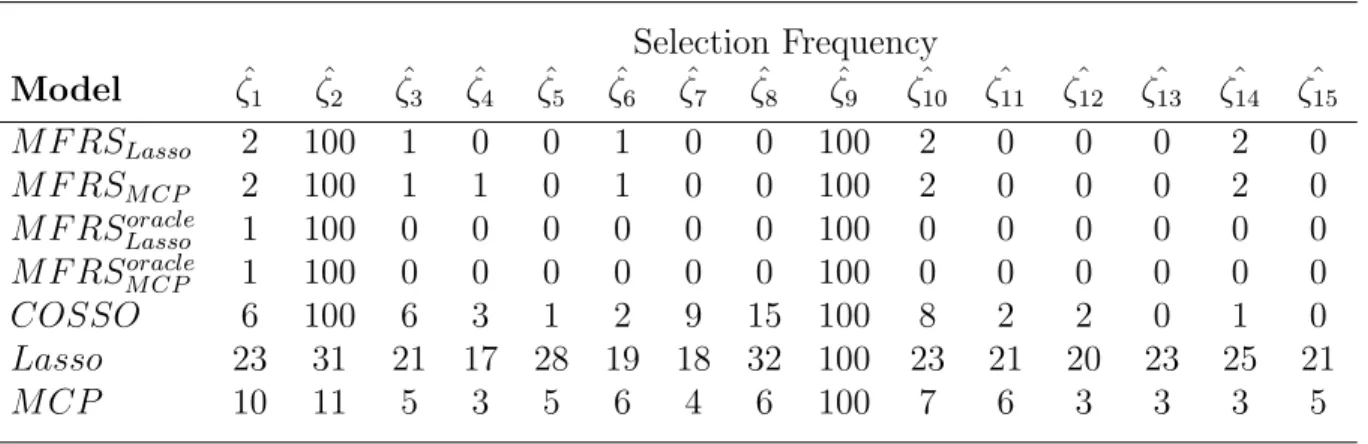
Table 2.3: FPC Selection for Scenario 1 Selection Frequency Model ζˆ1 ζˆ2 ζˆ3 ζˆ4 ζˆ5 ζˆ6 ζˆ7 ζˆ8 ζˆ9 ζˆ10 ζˆ11 ζˆ12 ζˆ13 ζˆ14 ζˆ15 M F RSLasso 2 100 1 0 0 1 0 0 100 2 0 0 0 2 0 M F RSM CP 2 100 1 1 0 1 0 0 100 2 0 0 0 2 0 M F RSoracle Lasso 1 100 0 0 0 0 0 0 100 0 0 0 0 0 0 M F RSoracle M CP 1 100 0 0 0 0 0 0 100 0 0 0 0 0 0 COSSO 6 100 6 3 1 2 9 15 100 8 2 2 0 1 0 Lasso 23 31 21 17 28 19 18 32 100 23 21 20 23 25 21 M CP 10 11 5 3 5 6 4 6 100 7 6 3 3 3 5

Estimated marginal plot with 95 percent shaded confidence bands of the function

hevaluated at 100 grid points for each component while holding all other components equal to 0.5 in Scenario 1.

(46)

Setting of Scenario 2: In this scenario, the objective was to assess the performance of our method on both functional sparsity and within functional sparsity. Because of this complexity, we reported detailed numerical results in the main text of this paper. Here for each subject i, we generated 4 functional predictors {Z1

i,· · · , Zi4} of the

form: Z`₍_t_{) =}P9 j=1

√

ςjξjφj(t), ` = 1, . . . ,4, where φj, ςj, and ξj are set at the same

values as those given in Scenario 1. It follows that #»z = (ζ1

1, . . . , ζ91, . . . , ζ14, . . . , ζ94)> where ζ_j` is the jth transformed feature for the `’th functional covariates. To specify sparsity, we chose the first and second functional covariates, Z1 and Z2, by relating the transformed FPC features, {ζ1

1, ζ31, ζ41, ζ22, ζ72}; they are the first, third and fourth features from the first functional and the second and seventh from the second func-tional covariate, which will be related to the outcome in a non-linear and non-additive way:

(47)

yi = 2xi+ζi11+ζ 1 i3+ζ 1 i4+ζ 2 i2+ζ 2 i7+ 10 cos(2πζ_i1₁)−10 ζ_i2₂2+ 10 ζ_i2₇2 −10 ζ_i1₃2+ 10 exp(−ζ_i1₃)ζ_i1₄−8 sin(2πζ_i2₇) cos(2πζ_i1₃) + 20ζ_i1₁ζ_i2₇+i

where i iid

∼ N(0,1) and ζ`

ij is the jth transformed score for the `th functional

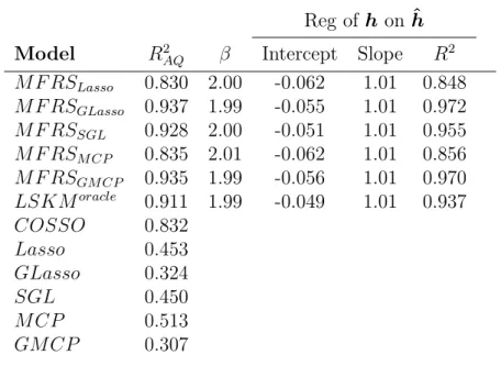
pre-dictor for subject i. In this scenario, we set up both group sparsity (with only 2 of the 4 functional predictors being used) and within-group sparsity (with less then 9 of FPC features being used). In addition, we designed a non-additive structure in the true model across multiple functional covariates. We considered linear models, COSSO method for functional additive regression and oracle methods in the com-parison. From Table 2.4 regarding the goodness of fit, we see that all of our MFRS estimators outperformed the standard linear estimators in terms of R2

AQ among all

of our penalty functions and it outperformed COSSO for penalties that account for group sparsity. COSSO tended to perform on par for penalties that do not account for group sparsity (LASSO and MCP). It is evident that using a group sparsity penalty function (SGL, GLasso, and GMCP) clearly outperformed the methods that did not regularize grouping of covariates (Lasso and MCP). In addition, our estimators per-formed as well as the oracle LSKM estimator both in terms of R2

AQ and in terms of

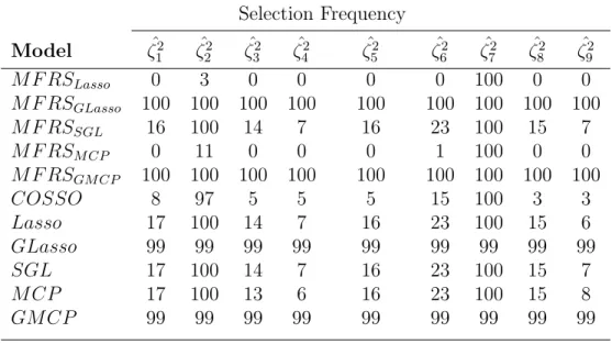
our estimate of h. The results also indicate that there were little differences between using a concave (MCP or GMCP) penalty function or using a convex (Lasso, GLasso or SGL) penalty function. In regard to the group sparsity, Table 2.5 indicates that the all methods had high sensitivity of detecting functional signals, while the proposed MFRS methods had better specificity than the linear models and the COSSO. Con-cerning the within group sparsity, it is interesting to note that a bigger difference is seen in terms of what type of penalty function is being used in model selection. Using

(48)

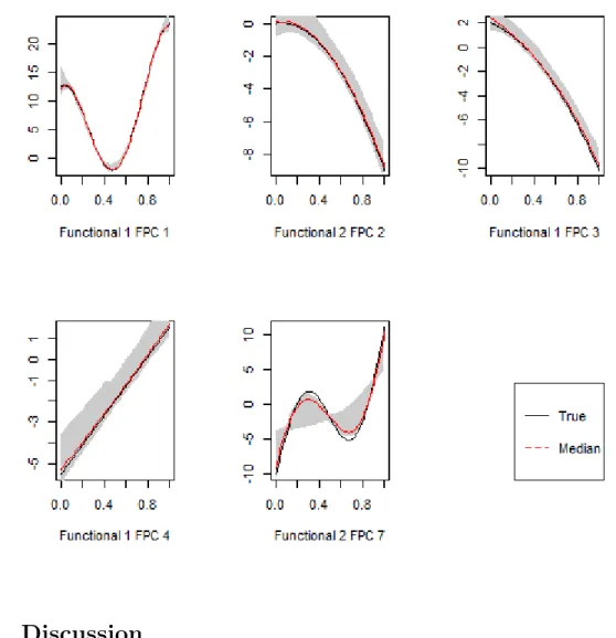
a general penalty (e.g. Lasso and MCP) that does not take the grouping structure into account tends to under-select specific members within a group as shown in tables 2.6 and 2.7. COSSO tended to perform well within group sparsity. Figure 2.1 shows that the MFRS method estimated the signal functions (Z1 _and _Z2_{) well.}

Table 2.4: Goodness of Fit via the concordance regression for Scenario 2 Reg of hon ˆh

Model R2_AQ β Intercept Slope R2

M F RSLasso 0.830 2.00 -0.062 1.01 0.848 M F RSGLasso 0.937 1.99 -0.055 1.01 0.972 M F RSSGL 0.928 2.00 -0.051 1.01 0.955 M F RSM CP 0.835 2.01 -0.062 1.01 0.856 M F RSGM CP 0.935 1.99 -0.056 1.01 0.970 LSKMoracle _0.911 _1.99 _-0.049 _1.01 _0.937 COSSO 0.832 Lasso 0.453 GLasso 0.324 SGL 0.450 M CP 0.513 GM CP 0.307

Table 2.5: Sensitivity and Specificity of Functional Selection for Scenario 2 Selection Frequency Model Zˆ1 _Zˆ2 _Zˆ3 _Zˆ4 M F RSLasso 100 100 0 0 M F RSGLasso 100 100 4 4 M F RSSGL 100 100 0 0 M F RSM CP 100 100 0 0 M F RSGM CP 100 100 3 4 COSSO 100 100 5 6 Lasso 100 100 19 21 GLasso 94 99 7 8 SGL 100 100 19 18 M CP 100 100 20 19 GM CP 93 99 7 8

(49)

Table 2.6: FPC Selection for Scenario 2 Functional Z1 Selection Frequency Model ζˆ1 1 ζˆ21 ζˆ31 ζˆ41 ζˆ51 ζˆ61 ζˆ71 ζˆ81 ζˆ91 M F RSLasso 100 1 97 0 0 0 0 0 0 M F RSGLasso 100 100 100 100 100 100 100 100 100 M F RSSGL 100 21 100 71 26 20 17 16 15 M F RSM CP 100 1 99 1 0 0 0 0 0 COSSO 100 2 100 93 1 0 0 1 0 M F RSGM CP 100 100 100 100 100 100 100 100 100 Lasso 100 10 100 100 10 8 7 10 5 GLasso 94 94 94 94 94 94 94 94 94 SGL 100 12 100 100 10 8 8 11 5 M CP 100 10 100 100 9 8 9 7 5 GM CP 93 93 93 93 93 93 93 93 93

Table 2.7: FPC Selection for Scenario 2 Functional Z2 Selection Frequency Model ζˆ2 1 ζˆ22 ζˆ32 ζˆ42 ζˆ52 ζˆ62 ζˆ72 ζˆ82 ζˆ92 M F RSLasso 0 3 0 0 0 0 100 0 0 M F RSGLasso 100 100 100 100 100 100 100 100 100 M F RSSGL 16 100 14 7 16 23 100 15 7 M F RSM CP 0 11 0 0 0 1 100 0 0 M F RSGM CP 100 100 100 100 100 100 100 100 100 COSSO 8 97 5 5 5 15 100 3 3 Lasso 17 100 14 7 16 23 100 15 6 GLasso 99 99 99 99 99 99 99 99 99 SGL 17 100 14 7 16 23 100 15 7 M CP 17 100 13 6 16 23 100 15 8 GM CP 99 99 99 99 99 99 99 99 99

(50)

Figure 2.1: Estimated marginal functions with 95 percent shaded confidence bands of the function h evaluated at 100 grid points for each component while holding all other components equal to 0.5 in Scenario 2

2.7 Discussion

In this chapter we proposed a method to model the non-linear relationship be-tween multiple functional predictors and a scalar outcome in the presence of other scalar confounders. We used the FPCA to decompose the functional predictors for feature extraction, and used the LSKM framework to model the functional relation-ship between the outcome and components. We developed a simultaneous procedure to select the important functional predictors and important features within selected functionals. We proposed a computationally efficient algorithm to implement the