Context-aware Background Application Scheduling in Interactive Mobile Systems

(1)

저작자표시-비영리-변경금지 2.0 대한민국 이용자는 아래의 조건을 따르는 경우에 한하여 자유롭게 l 이 저작물을 복제, 배포, 전송, 전시, 공연 및 방송할 수 있습니다. 다음과 같은 조건을 따라야 합니다: l 귀하는, 이 저작물의 재이용이나 배포의 경우, 이 저작물에 적용된 이용허락조건 을 명확하게 나타내어야 합니다. l 저작권자로부터 별도의 허가를 받으면 이러한 조건들은 적용되지 않습니다. 저작권법에 따른 이용자의 권리는 위의 내용에 의하여 영향을 받지 않습니다. 이것은 이용허락규약(Legal Code)을 이해하기 쉽게 요약한 것입니다. Disclaimer 저작자표시. 귀하는 원저작자를 표시하여야 합니다. 비영리. 귀하는 이 저작물을 영리 목적으로 이용할 수 없습니다. 변경금지. 귀하는 이 저작물을 개작, 변형 또는 가공할 수 없습니다.

(2)

Master's Thesis

Context-aware Background Application Scheduling

in Interactive Mobile Systems

Euijin Jeong

Department of Computer Science and Engineering

Graduate School of UNIST

2019

(3)

Context-aware Background Application

Scheduling in Interactive Mobile Systems

Euijin Jeong

Department of Computer Science and Engineering

(4)

(5)

(6)

Abstract

Each individual's usage behavior on mobile devices depend on a variety of factors such as time, location, and previous actions. Hence, context-awareness provides great opportunities to make the networking and the computing capabilities of mobile systems to be more personalized and more efficient in managing their resources. To this end, we first reveal new findings from our own Android user experiment: (i) the launching probabilities of applications follow Zipf's law, and (ii) inter-running and running times of applications conform to log-normal distributions. We also find contextual dependencies between application usage patterns, for which we classify contexts autonomously with unsupervised learning methods. Using the knowledge acquired, we develop a context-aware application scheduling framework, CAS that adaptively unloads and preloads background applications for a joint optimization in which the energy saving is maximized and the user discomfort from the scheduling is minimized. Our trace-driven simulations with 96 user traces demonstrate that the context-aware design of CAS enables it to outperform existing process scheduling algorithms. Our implementation of CAS over Android platforms and its end-to-end evaluations verify that its human involved design indeed provides substantial user-experience gains in both energy and application launching latency.

(7)

(8)

List of Figures

1 Daily network usage of the Facebook app and its corresponding state either being in the foreground or background. The Facebook app incurs background network traffic even when the user is not interacting with it. ---2

2 Measured power consumption of a popular game application for foreground and background states in a Galaxy Note 2 smartphone. ---2

3 The process states defined in Android [28] (left) and our simplified three states (right). ---7

4 Our simplified states and transitions between a pair of states. ---7

5 Our slotted time model of off and on periods (bottom) and an example of corresponding sets of background applications at each slot by LMK (top). ---8

6 The percentage of states (importance) in recorded logs (top) and the number of running processes at a moment and the number of unique processes (bottom). The numbers (-%) in the top graph indicate the average portion of each state across all participants (This figure is best viewed in color). ---10

7 Foreground activity of user 59 over two weeks (week 1 in Feb. 5-11 (top), and week 2 in Feb. 12-18 (bottom)). Regular temporal patterns are observed in weekdays and in weekends. ---10

8 The CCDF (complementary cumulative distribution functions) of off (left) and on (right) period distributions in week 1 and week 2 of user 59. ---11

9 The CCDF and the corresponding log-normal fittings of off (left) and on (right) periods of one randomly chosen user. ---11

10 The CDF of average off (left) and on (right) periods of users. ---12

11 Off (top) and on (bottom) failure rates of users. The length of a time slot is one second. The dotted lines are failure rates of each individual user. ---12

(10)

distribution fitting for the average launching probability (right). The frequently used applications of each user are not identical. The dotted lines are for each individual user. ---14

13 Memory (top) consumption in background and foreground, and cold/warm launch latency (bottom) of popular applications in 5 categories (Game, Messaging, Browsing, Portal/Video, Social). ---14

14 The conditional launching probability of applications (Xk) for a previously used application (Xk−1) in

each week of user 59. ---16

15 The overall architecture of CAS and its operations over time. ---17

16 A sample off-period classification by “active” (8am - 11pm) and “’inactive” (11pm - 8am) hours obtained from the first week trace (top) of one user. The classification obtained from the first week is applied to the second week (bottom) and it still shows a good match from regularity in human behaviors. ---18

17 CDF of prediction errors for off (left) and on (right) periods of users. ---19

18 Comparison of scheduling algorithms. The error bars indicate 25th and 75th percentiles. ---31

19 Background application schedules of CAS for one user in off periods. The x-axis is in log scale. We list the application names of the ordered sequence in the graph and the numbers (-%) indicate the launching probabilities. 1: Messaging, 2: Browsing, 3, 5: Social, 4: Navigation, 6: Contacts, 7: Utility. ---32

(11)

List of Tables

1 Logged events and associated fields. ---9

2 The portion of user-triggered launches, average running times of 12 most popular applications and their top-1 to top-3 probabilities across all users. ---13

3 Summary of major notation. ---21

4 Summary of contextual information. ---30

5 Comparison of scheduling algorithms. ---35

(12)

1

Ⅰ. Introduction

As mobile devices have become an essential part of our lives, people expect more capability from them such as longer battery life, ubiquitous access to Internet, immediate response time, and fresh contents (e.g., messages, feeds, news, ads, sync data, or software updates). The recent advancement of cellular networks and cloud computing is partly fulfilling these needs. However, certain performance features such as long battery life and high quality-of-service (e.g., low latency and fresh contents) have intrinsic tradeoffs that make it difficult to optimize simultaneously.

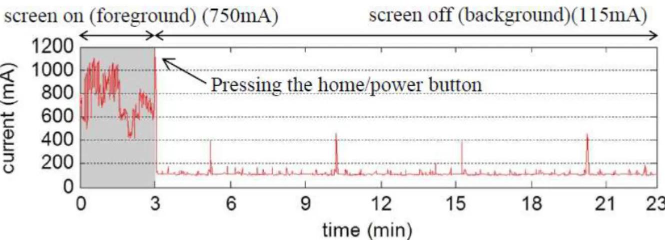
In a large-scale measurement study of 2000 Galaxy S3 and S4 devices by Chen et al. [2], [3], 45.9% of the total energy drain occurs during screen off periods. This high energy consumption mainly comes from background applications that update contents, collect user activity information, or keep components in active states [4], [5]. However, these background activities may not be always beneficial for users. For example, if a social network application updates its contents frequently (say every 20 minutes), but the user launches this application once a day, then most updates unnecessarily waste network energy.1 _{As a motivational example, we show the measured daily network usage}2 _{of a}

Facebook application on a Galaxy S7 smartphone running Android 6.0.1 in Fig. 1, where the update or collection intervals are less than 20 minutes.3 _{Also, gaming or map applications often keep high}

power-consuming components such as CPU and GPS in active states while being in background. This operation is intended to provide immediate responses from those applications but wastes energy unless the user re-launches them within a short time. This inefficient stand-by operation is indeed observed in a popular game application, as shown in Fig. 2. To this end, we aim at managing mobile applications in a resource-efficient manner by exploiting per-user application usage behaviors analyzed in the perspective of contextual usage statistics. It is important to mention that managing applications not only influences the computing behaviors but also the networking behaviors of a mobile system which in turn leads to further resource optimizations such as delaying or suppressing non-urgent background network traffic.

To our knowledge, the most widely used application controller in Android [8] and iOS [9] is called

1_{It is well known that frequent network traffic incorporates large ramp and tail energy overheads [6], [7].} 2_{We log network usage by reading /proc/uid_stat/[uid]/.}

3_{The authors in [4] revealed that the Facebook application uses network data every 5 minutes or every 1 hour in their large}

scale measurement between Dec 2012 to Nov 2014. They also revealed that network traffic from background applications consumes 84% of total network energy, mainly due to periodic contents updates and their tail energy consumption.

(13)

2

Fig. 1. Daily network usage of the Facebook app and its corresponding state either being in the foreground or background. The Facebook app incurs background network traffic even when the user is not interacting with it.

Fig. 2. Measured power consumption of a popular game application for foreground and background states in a Galaxy Note 2 smartphone.

the low memory killer (LMK) that commonly kills (i.e., unloads or terminates) applications to secure more available memory. Popular memory kill algorithms that are often implemented with LMK purge applications in the order of either LRU (least recently used) or process priority [10]. As this mechanism is merely inherited from computer systems with abundant resources (e.g., energy), it never considers contextual information of application usages. Thus, it naturally fails to manage mobile applications in an efficient way.

There have been two complementary approaches to tackle this problem. Several papers [11]–[14] tried to identify energy bugs/hogs, that mainly come from coding errors. This may successfully kill all detected buggy activities, but benign operations such as activity logging can also be stopped (false

(14)

3

positive) and unnecessary network activities may be mostly intact (false negative). Another recent approach in [2] proposed a metric called BFC (Background to Foreground Correlation) to quantify the level of user engagement for each application on the fly. If the BFC value is smaller than a threshold, background activities are implemented to be suppressed. [2] also developed HUSH that puts applications that have not been recently used in foreground into inactive states, and extends the duration of being in the inactive states in an exponential manner. They showed that the screen-off energy saving of their algorithms is 15-17% in their large-scale traces.

The second approach partly tackled the energy-inefficient activities, but still this approach is myopic as it ignores the very important statistics on when the user will relaunch an application. As human behaviors have regular patterns in their daily lives, it is clearly possible to design a more efficient application controller that is far beyond the naive exponential mechanism. This is only possible when deeper understandings of per-user and per-application usage behaviors are acquired.

To that end, we collect application usage of 103 Android users for which we deployed a logger that was designed to periodically send detailed application, sensor, and memory usage data to our server. The total data collected spans over 1057 days and reaches about 20GB. We find that the usage patterns follow heavy tail distributions: (i) The launching probabilities of applications follow the Zipf’s law, and (ii) inter-running and running times of applications resemble log-normal distributions. We also reveal detailed context-dependency in the re-launching probabilities, which convey more personalized control ideas over existing studies [15]–[19]. To realize a control algorithm that exploits such personalized

context-dependency, we automate the procedure of per-user context extraction by adopting unsupervised learning methods that significantly improve prediction accuracy.

With the contextual knowledge, we propose a new application control framework, CAS (Context-aware Application Scheduler) that works by predicting when a user will launch an application and which

application will be used. Trace-driven simulations with consideration of system overhead show that CAS outperforms the Android genuine resource scheduler, LMK, and Android 6.0. We also verify the practicality of CAS by implementing the system on Android.

(15)

4

Ⅱ

. Related Work

We classify previous work on mobile resource scheduling into several categories from experimental studies to implementations and summarize their contributions.

Human behaviors on mobile application usage: To establish the foundation of context-awareness for mobile resource scheduling, several pioneering experimental studies [15]–[21] have been performed to analytically understand how humans use applications given contexts such as time/location information, and the last used application. Falaki et al. [21] studied usage traces from 255 users and found that the levels of activities are vastly different across users. They also found that screen off times fit well with the Weibull distribution.

Application preloading algorithms: Those early studies on context-awareness led to the development of application preloading/prefetching algorithms [22]–[26] applications that substantially reduce the perceivable start-up latency (i.e., launch latency) by preparing required resources (including computation such as rendering, and communication such as feed updates) before they are requested by users. However, most previous studies have focused on which application a user will launch next, but not on when the user will launch it. [23] is the only work that concerned the moment of launching, but the authors did not consider the cumulative penalty of preloaded applications, hence their prefetching schedules may suffer from large energy wastage until the predicted application is actually accessed.

Application unloading algorithms: The default low memory killers (LMK) on Android [8] and iOS [9] unload or terminate applications to secure more memory resource, when the available memory goes below a pre-defined threshold. Popular memory kill algorithms that are often implemented with LMK purge applications in the order of either LRU (least recently used) or process priority [10]. Android version 6.0 (Marshmallow), released in October 2015, adopts features called App standby and Doze

mode [27] for energy saving. App standby suppresses background activities of an application that has not been used in foreground for 3 days. The Doze mode is enabled when a user leaves the device for a certain amount of time. Doze mode restricts background apps’ access to network and CPU for most of time, and lets background apps complete their activities for a short maintenance window. Doze mode schedules this maintenance window less frequently as the untouched period gets elongated.

A recent paper [2] proposed simple unloading algorithms called BFC (Background to Foreground Correlation) and HUSH for screen-off background activities. The BFC metric quantifies the likelihood that a user will interact with an application during a next screen-on interval after its background

(16)

5

activities. BFC updates the metrics using an exponential moving average at the end of each screen on period, and unloads applications if their BFC metrics are less than a cutoff value α. Another algorithm, HUSH increases the suppression interval of an application if it has not been used in foreground using exponential backoff (i.e., the interval is multiplied by a given scaling factor σ). Once an application is used in foreground, the interval is reset to an initial value. This simplistic algorithm is shown to save about 15-17% of energy in their large-scale usage traces. Our preliminary work [1] was the first of its kind that jointly considers preloading and unloading of background applications. However, the scheduling algorithm therein was not able to systematically find an optimal schedule for a given resource constraint (e.g., energy, or launching latency).

(17)

6

Ⅲ

. Preliminary

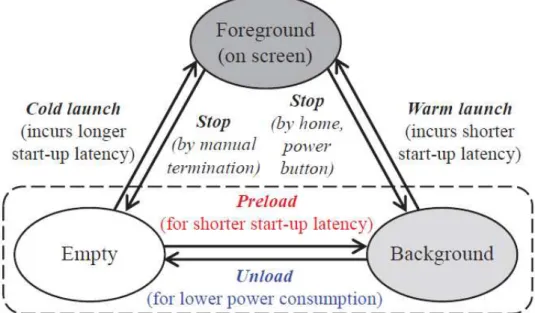
In this section, we explain basic concepts for application processes. In Android OS, there are various application states each of which has its corresponding “process importance” ranging from 100 to 1000 [28]. An Android application4 _{installed on a device stays in one of the states at a time slot. Fig. 3 shows}

all the states defined in Android and our simplified mapping of those states into three states: foreground,

background, and empty. We define a foreground process to be a process in use and that is visible to users. By the definition, there can be at most one application in foreground at each time. An empty

process5 _{is defined to be a process unloaded from memory, and thus no resource is allocated to that}

process. We denote a background process as a process that is loaded but not running on foreground.

The rationale behind our simplification of states is that the processes that are running with no foreground UI on the screen show similar resource consumption characteristics (e.g., memory and power) as background processes of importance 400 rather than foreground processes running on the screen. Also, these processes can be unloaded just like background processes of importance 400 without disrupting on-going user experience, except system processes (e.g., phone caller and application launcher) that are designed to be running all the time, and user-interactive applications (e.g., music, radio and recorder) that are usable even without visible UIs.

We depict the transitions between states in Fig. 4. An empty to foreground transition called cold launch occurs when a user touches an empty (i.e., unloaded) application to launch. A transition from background to foreground called warm launch is mostly made when a user chooses to use the application by relaunching an application that is still kept in the background, and thus has shorter latency than cold launch but consumes memory and battery for background activities. Therefore, user experience on battery life and application launch latency is highly dependent on the decision of putting an application in either of background or empty state.

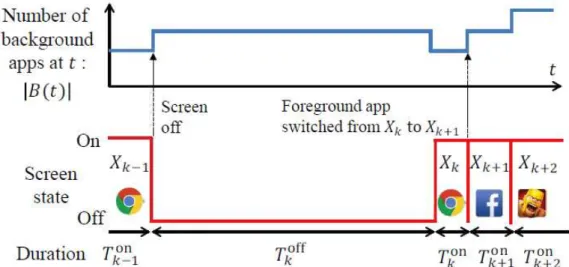
We further define the system state as either of off or on and its period. Tkoff denotes the k-th

screen-off period when all applications are either in background or empty, while Tkon denotes the k-th

screen-on period for which an applicatiscreen-on is being used in the foreground. Fig. 5 depicts how the number of background applications (|B(t)|) changes as the screen state and foreground application Xk change over

time, under the Android default scheduler LMK, where B(t) and Xk denote the list of background

4_{We interchangeably use process and application.} 5_{The empty state corresponds to}_suspend_{in iOS [9].}

(18)

7

Fig. 3. The process states defined in Android [28] (left) and our simplified three states (right).

Fig. 4. Our simplified states and transitions between a pair of states.

applications at time t and the foreground application at k-th screen on period. Under LMK, a foreground process goes to background when the user switches to a different foreground application or turns off the screen. LMK kills applications in background in the descending order of importance values when the available memory goes below multiple levels of preset memory thresholds. This is surely done with no consideration on when the killed application is going to be relaunched. Thus, LMK results in higher cold launch probability, even though it keeps a number of applications in background and brings high energy wastes.

(19)

8

Fig. 5. Our slotted time model of off and on periods (bottom) and an example of corresponding sets of background applications at each slot by LMK (top).

(20)

9

Ⅳ

. Measurement Study

4.1. Data Collection

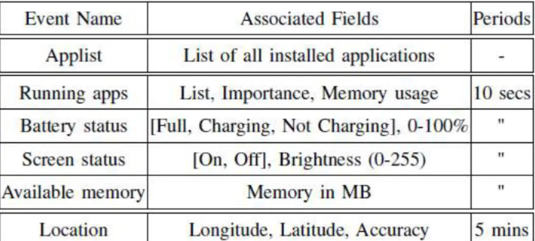
To capture application usage behaviors of smartphones in the wild, we performed our own data collection with 96 Android users selected from a few popular Internet communities of South Korea during two weeks in Feb. 5-18, 2015. We provided a data logger programmed to periodically record application usage and device characteristics summarized in Table 1, and upload the data to our server daily. We anonymized all user information and IDs at the level of user devices. We asked users not to use task killers and not to manually unload applications while participating our experiment, in order to see how the Android genuine scheduler, LMK works. The average valid data per user is about 11 days, and the total data size is about 20GB. We also asked the participants to fill an anonymized survey involving occupation, age band, gender, and personal statement on their dissatisfaction of the smartphone (e.g., latency, freeze), summarized in our survey report [29]. To improve the reliability of the responses we did our best to create an anonymous interface to give them confidence in providing the correct information. Participants come from diverse occupations, genders, ages, and devices (e.g., Samsung Note2, Note3, Note4, S3, S4, S5, LG G2, G3). Most of participants use Android KitKat (4.4.2) (75%), where a small number of them use Jelly Bean (4.2.2 and 4.3) and Lollipop (5.0.1). From our survey, short lifetime, frequent freezes, and long start-up latency were still the major problems for participants, even though their smartphones were mostly state-of-the-art.

Table 1. Logged events and associated fields.

4.2. Key Observations from the Measurements

(21)

10

Fig. 6. The percentage of states (importance) in recorded logs (top) and the number of running processes at a moment and the number of unique processes (bottom). The numbers (-%) in the top graph indicate the average portion of each state across all participants (This figure is best viewed in color).

Fig. 7. Foreground activity of user 59 over two weeks (week 1 in Feb. 5-11 (top), and week 2 in Feb. 12-18 (bottom)). Regular temporal patterns are observed in weekdays and in weekends.

Application usage statistics of users and states: In Fig. 6, we plot the fraction of time spent in different process importance evaluated from our experimental logs, the number of running processes at a moment, and the number of unique processes that have ever been used during the experiment. We treat system and user-interactive (e.g., music) processes separately in the figure. We find that the number of running (foreground+background) processes per user is 5.2 on average, and the number of unique processes ever used per user is 55.1 on average, excluding system and user-interactive processes. 73% of unique processes have not been used in foreground for more than 3 days in our traces, and these processes will be unloaded by the feature App standby6 _{of Android 6.0 released in late 2015, which suppresses}

background activities of an application that has not been used in foreground for 3 days. However, the number of corresponding background processes in run is only 2 on average (40% of that in LMK) so that the energy saving from this feature is not significant as we will see in our simulation section. The fraction of time a process spends in the foreground state is about 6% on average, while the fraction of time in background is about 16 times of being in foreground. The fraction of time that the screen is on is 21% on average (i.e., 5 hours per day).

Regularity in application usage: The existence of the regularity of application usage patterns of a person is the key to make a mobile system predictive, and thus more efficient. In order to understand individual application usage patterns, we investigate the timings of all foreground application actions

(22)

11

Fig. 8. The CCDF (complementary cumulative distribution functions) of off (left) and on (right) period distributions in week 1 and week 2 of user 59.

Fig. 9. The CCDF and the corresponding log-normal fittings of off (left) and on (right) periods of one randomly chosen user.

(launching/stopping) and analyze the event intervals. For the visualization, we choose one user randomly and depict the timings of the application launches for two consecutive weeks in Fig. 7. We observe that the active hours are highly regular and the intensity of activities during the weekdays or weekends for two weeks resemble each other. More specifically, we find that there exists strong distributional similarity in both off and on periods in the first week and the second week, as shown in Fig. 8. These results confirm that temporal and distributional knowledge from usage history can be used to better predict the future application usage.

Off/on period distribution: In Fig. 9, we fit off/on period distributions of a randomly chosen user to show that the distributions are heavy-tailed. We verify by Cramer-Smirnov-Von-Mises (CSVM) [30] and Akaike [31] tests that off/on periods of all users have the best fit with log-normal distributions7

7_{The probability density function (PDF) of the log-normal distribution with parameters}_μ_and_σ_is

(23)

12

Fig. 10. The CDF of average off (left) and on (right) periods of users.

Fig. 11. Off (top) and on (bottom) failure rates of users. The length of a time slot is one second. The dotted lines are failure rates of each individual user.

rather than exponential, Weibull, truncated Pareto, gamma and Rayleigh distributions. We use the best fitting log-normal distributions as representative of off/on periods in the following sections for tractability. We also depict the CDFs of average individual off/on period of users in Fig. 10. The average individual off period in total is 15.5 mins for a whole day, 13.5 mins for the active hours (9:00 to 24:00) and 33.8 mins for the inactive hours (24:00 to 9:00). Not surprisingly, the off period in the inactive hours is much longer than in the active hours, as users tend to leave the device unattended during the inactive hours. The average individual on period is about 1.4 mins.

(24)

13

Table 2. The portion of user-triggered launches, average running times of 12 most popular applications and their top-1 to top-3 probabilities across all users.

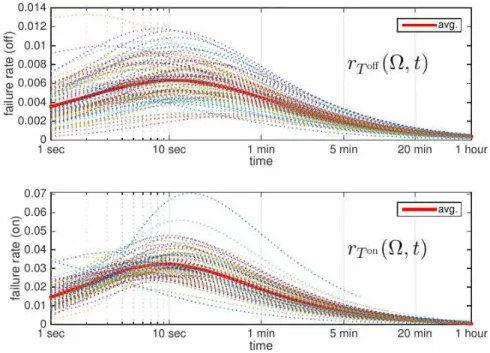
frequency of altering its state from “off to on” (launching) or from “on to off” during off/on periods at the elapsed time t, which is commonly called as the failure rate. Formally, the failure rate of T is  (t) ≜

_()

(), for t such that FT (t) < 1, where fT (t) and FT (t) = P[T ≤ t] are the probability mass function and

cumulative distribution function (CDF) of T, respectively. T can be either T off _or_Ton_{. We call off failure}

rate (from off to on) for T off _{and on failure rate (from on to off) for}_Ton_{. In Fig. 11, we plot off and on}

failure rates, for each user (dotted lines) and on average (solid line). For most of users, the off and on failure rates increase at first but soon decrease right after 10 seconds. The pattern of having decreasing failure rate over time is called negative aging [32]. This indicates that users are less likely to launch an app as the off or on period increases. Thus, an energy-efficient control needs to reduce background activities as the failure rate starts to get reduced. This also suggests that the increasing backoff mechanisms of HUSH [2] and Doze [27] can be effective although their schedules are neither optimized nor personalized given that the individual failure rates (dotted lines in Fig. 11) show distinct characteristics for different users.

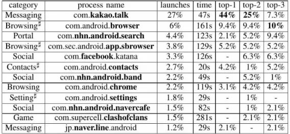
Frequently used applications: In Table 2, we summarize the 12 most popular applications across all participants from the perspective of the launching probabilities, average running times and 1 to top-3 probabilities. Top-n probability of an application is defined as the probability that the application is the n-th most frequently used application of a user. The most popular application in our experiment is shown to be KakaoTalk (com.kakao.talk), a messaging application known as used by 93% of smartphone users in South Korea as of May 2014. 95% of our participants use KakaoTalk.

(25)

14

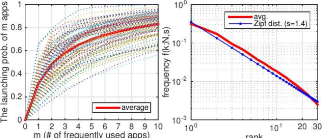
Fig. 12. The CDF of the launching probability of m most frequently used applications (left) and Zipf distribution fitting for the average launching probability (right). The frequently used applications of each user are not identical. The dotted lines are for each individual user.

Fig. 13. Memory (top) consumption in background and foreground, and cold/warm launch latency (bottom) of popular applications in 5 categories (Game, Messaging, Browsing, Portal/Video, Social).

applications are individually sorted. We find that the launching probability follows Zipf’s law8 _with

exponent s = 1.4, and the aggregated launching probability of the 10 most frequently used applications of a user is more than 80% on average. Recall that the average number of unique applications ever used for a user is 55.1. Therefore, users tend to use a small fraction of the applications most of the time, and there is little gain in the start-up latency and related user experience when infrequently used applications are kept in background.

Memory consumption: The average physical memory size of experimented smartphones is 2.14GB. From the log, we find that the available memory is 488MB on average, which is only 22.8% of the physical memory (90% of users have less than 31.6% of total memory available). This is mainly from the memory threshold of the low memory killer, below which it terminates applications. The lack of

8_{The frequency of elements of rank}_k_,_f(k;s,N)_{of a population of}_N_{applications is proportional to}_k-s_{, where}_s_{is the exponent}

(26)

15

free memory may freeze a mobile device frequently and degrade user experience. The average memory consumption of a controllable activity process is 55.4MB in background and 116MB in foreground. We depict memory consumption of 25 popular applications (5 applications in Game, Messaging, Browsing,

Portal/Video, Social categories) in foreground and background in the top of Fig. 13. The memory consumption in background is almost half of that in foreground, so that a mobile device lacks available memory if many applications are running in background. The time averaged memory size from controllable activity processes in background is 325MB. Note that the mobile OS and system processes occupy 60% of physical memory on average.

Warm and cold launch latency: In the bottom of Fig. 13, we present warm and cold launch latencies for the popular applications measured from our controlled experiment using Samsung Note2. To quantify the launch latency, we first measure the time durations until (1) screen rendering, and (2) loading application data in memory is completed, by filtering and monitoring Android logcat debugging outputs [33]. All other applications are unloaded before each measurement. We then regard the maximum of these two time durations as the launch latency. The average warm and cold launch latencies are 0.9s (rendering: 0.7s, memory loading: 0.4s) and 4.5s (rendering: 3.61s, memory loading: 3.58s), respectively. The game applications show the most drastic difference in latency, where the warm and cold launches take 12.6s and 1.8s, respectively. This is mostly due to loading high volume of texture data onto memory and rendering initial game scenes. For the tested popular applications, application preloading that transforms a cold launch into a warm launch decreases the start-up latency by 80% (3.6s).

User survey: We summarize key results from our survey. We first asked participants to choose major problems in their smartphones. 71% of participants chose short battery lifetime and 40% of them chose frequent freezes. Also, 46% of participants experience inconvenience from long start-up latency at least once a week. The battery lifetime that participants experience when it is fully charged is 9 hours on average, where it ranges from 3 to 24 hours. To increase battery lifetime and mitigate freezes, 82% of participants manually terminate applications and 28% of them use application killer software (e.g., Advanced Task Killer [34]). We also requested participants to list the applications with long startup latency and the length of perceived latency they experienced. More than 77% of participants have provided at least one application with long startup latency. The average startup latency of them is 7.3 seconds, where that of gaming applications is 9.1 seconds (and messaging: 3s, social: 3.6s, browsing: 6.3s, navigation: 6s). Thus, short lifetime, frequent freezes, and long start-up latency are still the major problems for smartphone users, even though their smartphones are almost state-of-the-art.

(27)

16

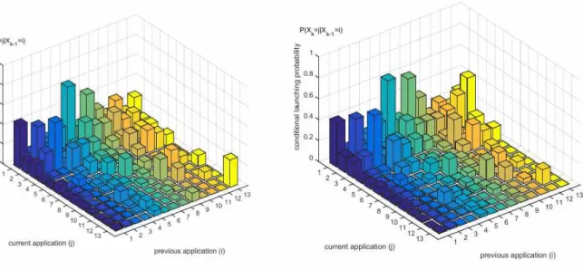
Context dependency: We also analyze app usage patterns incorporated under various contexts. Here, contexts correspond to any information that characterizes the situation of users, which enables us to predict future app/component invocations more accurately. In Fig. 10, the average inter-launching time at inactive hours (24:00 to 9:00) is about 3.6 times longer than the average inter-launching time at active hours. In Table 2, we find that the average on periods are vastly different across applications (e.g., long running time for games and browsers, and short running time for messengers). In Fig. 14, we depict the conditional launching probability of applications (Xk) for the previously used application (Xk−1), for one

user in each week. The application index is sorted by the launching frequency in descending order (application 1 is the most frequently launched application). We choose 13 popular applications for visibility. We note that if there is a non-zero screen-off period between two consecutive on periods (Tk-1on and Tkon), Xk−1 and Xk could be the same application, and P[Xk = Xk−1|Xk−1] can be non-zero. We

observe that the launching probability is vastly different depending on the previous applications. These patterns are also quite similar in each week. Therefore, the likelihood of launching an application at a moment depends on the previous application, and these statistics can be learned from history. We also observe context dependencies such as the duration of the previous intervals (Tk-1off, Tk-1on). For instance,

after using a messaging app, the next inter-launching times are typically shorter than average, as the recipient of a message may respond quickly. We omit more details for brevity.

Fig. 14. The conditional launching probability of applications (Xk) for a previously used application

(28)

17

Ⅴ. System Architecture

Fig. 15. The overall architecture of CAS and its operations over time.

In this section, we propose our system design of CAS as depicted in Fig. 15. Our framework consists of three major components: 1) context monitor, 2) user profiler, and 3) background application controller. Over these system components, CAS runs in three phases: collection, pre-computation, and control. The collection phase builds personalized statistical information about application usage patterns such as described in Section IV. This data will be used in the pre-computation and control phases. The precomputation phase will be discussed in more detail with the algorithm descriptions in Section VI. Here, we overview how each component works sequentially.

Collection phase and context classification: In the collection phase, context monitor collects various contextual information in background, to build information base on application usage pattern. Contexts we collect are screen state, time and location information, memory and CPU/network usage, application launch sequence, and battery level. Using the information base, the user profiler analyzes per-application usage behavior, cross-correlations of per-application usage behaviors, and resource (power/memory) consumption of background applications according to component-wise power models

(29)

18

Fig. 16. A sample off-period classification by “active” (8am - 11pm) and “’inactive” (11pm - 8am) hours obtained from the first week trace (top) of one user. The classification obtained from the first week is applied to the second week (bottom) and it still shows a good match from regularity in human behaviors.

in [35], [36], with diverse statistical measures such as failure rates and launching probabilities. Collection of data for learning may take some time (e.g., one week) in order to prepare a reasonable amount of statistics at first (e.g., when a user buys a new phone).

To better exploit contexts, the collected context information of traces can be classified and labeled. For instance, time of a day can be roughly classified into two labels, active and inactive hours, which may show two distinct probabilistic distributions of off and on periods by the nature of human life cycles. The labels resulted from classifications of many contexts will lead to a condition for prediction, where the condition is composed of a tuple of context labels such as (time = Active, last app = Facebook). People have different lifecycles and habits, so that contexts should be classified individually. In order to classify contexts automatically in a personalized manner without asking users a manual classification, we adopt unsupervised learning techniques. Unsupervised learning aims at classifying input data autonomously by clustering the data by their correlation (i.e., similarity). For instance, when classifying “time of a day” into k continuous time blocks, we can setup the following clustering problem which minimizes the residual sum of square errors from the clustering.9_{We solve this problem using a}

k-means algorithm [37]. min  ∑:∈(− [| ∈ ])+ ∑ (− [| ∉ ])  :∉ ,

where Sk is time of a day of k-th sample (at the beginning), and HA is the active timezone that is

(30)

19

Fig. 17. CDF of prediction errors for off (left) and on (right) periods of users.

continuous (e.g., HA = [a,b], where a is 10:00 and b is 21:00). Sk ∈ HA if Sk is within the time interval of

HA. We depict an example of “time of a day” classification for off periods in Fig. 16. The diurnal pattern

of this user is clearly identified by the classification. We find that most of the users need only 2 continuous time blocks (i.e., k = 2) to describe their temporal activities and show very little gain from further separation.

In Fig. 17, we depict the residual sum of squares of users for off and on periods in the test set (i.e., the second week of the trace), where the contexts (time of a day, previous off and on periods, last used application) are trained from the first week of the trace. We note that these dependencies including diurnal patterns are vastly different among users depending on their usage patterns and lifestyles. The residual sum of squares is decreased by 29.8% and 40.3% for off and on periods on average, respectively. Thus, it is clear that our automatic context classification leads to more accurate prediction. We also find that the entropy10 _{of the next launching app,}_X

k, is substantially reduced as well, which is omitted for

brevity. Intuitively, lower entropy means reduced uncertainty and better predictability.

Pre-computation and control phases: Based on this analysis, the background application controller computes sets of background applications for possible combinations of contexts in both off and on periods, in the pre-computation phase. For each cluster C (i.e., a tuple of several contexts), we use the conditional distribution Tk|C and conditional probability of Xk|C where these conditional values are

trained under the cluster C. In other words, our algorithm (which will be explained in the next section) will run for each cluster C. Therefore, we exclude the conditional information C in the rest of the paper, i.e., Tk = Tk|C and Xk = Xk|C, for simplicity. This pre-computation happens once in a while (e.g., one time

per week) to adapt for the change of the application usage behavior. Pre-computation also runs during the inactive hours with the device connected to its charger, to avoid any inconvenience to users. During the control phase, at the start of each off or on period, the controller calls the context monitor and

10_{The entropy for an application launch is}_{− ∑} _[

= ] log[= ] ∈ .

(31)

20

acquires the contextual information at the moment as its input. Based on the pre-computed list of background applications at each moment for the given contextual information, background application controller executes pre/unloading during the on or off period. As the recommended list of background applications at each moment are pre-computed, these executions do not bring any computational burden.

(32)

21

Ⅵ

. Algorithm Design

In this section, we formulate a submodular optimization problem that selects the best set of background applications to minimize the total penalty in energy and start-up latency. Then, we develop a practical scheduling algorithm for CAS. We also develop an iterative algorithm that finds the optimal schedules for a given energy constraint. This constrained optimal scheduling is practically valuable to users who want the best application performance at each level of energy allowance.

6.1. System Model

Table 3. Summary of major notation.

System states: We summarize major notations in Table 3. We let Ω (|Ω| = N) denote the set of controllable applications of a user, which does not include any system and user-interactive processes. We define B(t) ⊆ Ω and (t) ⊆ Ω to be the sets of applications in the background and empty states, respectively, which are our main control knobs.

We define the system state as an off/on period as in Fig. 5. We denote Tkoff and Tkon as random variables

of the k-th off and on period, respectively. We denote Xk as the foreground application that runs during

the time duration of Tkon.11 We recall that the failure rate is defined as  (t) ≜_ ()

(), for t such that

FT (t) < 1. T can be either Toff or Ton. We also define the partial failure rates for a set of empty applications

(33)

22

(t) as (),  =  () ⋅ [ ∈ ()] , which quantifies the rate that one of empty applications (t)

is launched at t. Note that (Ω,t) = (t).

Power consumption and memory usage model: For applications included in Ω, we define a power function, : 2_{→ ℝ}

 and a memory function : 2→ ℝ that respectively represent the amount of

the average power and memory usage of a set of background applications. Based on the observations made in [35], we model P as a monotone submodular function12 _of_B₍_t_{). Our model is reasonable since}

applications share hardware components, and each of them becomes more power-efficient as the utilization becomes higher. We define Δ() = (⋃{}) − () as the marginal increase in power

consumption by adding an application i in the background application set B. A memory function M is a linear additive function13 _{for any}_B₍_t_{). Note that we use average power and memory consumption for}

long-term optimization. For simplicity, we model that the energy consumption for preloading and unloading is minor in the long-run and that the transition delay is much shorter than one time slot. These models practically make sense as the preloading/unloading consume its power less than a few seconds and happen only a few times an hour. More detailed discussion on the consumption of the transition energy will be provided in the simulation section.

6.2. Problem Formulation

We aim to develop a scheduling algorithm for CAS that reduces and balances energy consumption and user disutility from experiencing cold launch of applications, under a given memory budget Mth.

Since there is a trade-off between the energy consumption and the user disutility, we adopt a parameter  to treat both metrics as a unified measure. A user who is less sensitive to latency but is keen to extend battery lifetime will choose a smaller  value, and vice versa.14_{The optimal scheduling algorithm for}

CAS can be obtained from the optimization problem that minimizes both the energy consumption and the user disutility over the infinite time horizon. The optimization problem is formally defined below. We present the equation by the summation of two components corresponding to off and on period optimizations for better understanding.

min _(),∀ _{()}   + min _(),∀ _{()}    _{≜ ∑} _ℙ[ _{= ](∑} _{ }_{() +  ∙ ℙ[ ∉ }_()])    ,

12 _{( ∪ ) ≤ () + () − ( ∩ )}_for_{,  ⊂ Ω}_{, and}_{() ≤ ()}_{for any}_{ ⊆ }_. 13_{For any disjoint sets}_{,  ⊂ Ω}_,_{( ∪ ) = () + ()}_.

14_{We will discuss later in this section how}_γ_{can be automatically determined for a user who wants to limit either of energy}

(34)

23 H _{≜ ∑} _ℙ[ _{= ](∑} __{() + }_{∙ ℙ[ ∉ }_()])    , where  = ℙ[T off _{= 0]}_{, B}on₍_t₎_⊆_Ω

k, and Ωk = Ω \ {Xk}. We use Boff(t) and Bon(t) to denote the set

of background applications in an off and on period, respectively.

The optimization is decomposed into off and on problems (i.e., Hoff _and_Hon_{), each of which}

corresponds to the optimization during a screen-off or screen-on period. In the off-period optimization (Hoff_{), the summation of}_P₍_Boff₍_τ_{)) from}_τ_{= 1 to}_t_{indicates the energy consumption when the length of}

an off period is t and the second term quantifies the expected disutility from the cold launch of an application weighted by γ. In an on period, the disutility is multiplied by the probability that the user will switch to another application without going through an off period (i.e., ℙ[T off _{= 0]). Otherwise,}

the device will go into an off period (i.e., the user stops using the device) and there will be no disutility.

By restating energy and disutility terms in Hoff _using_ℙ_[_Toff _≥_t_{], we have} H _{= } _ℙ[ _{≥ ](} ()_{ +  ∙ }   (), )  

from the definition of the partial failure rate. Since we have assumed that the latency and energy overhead for preload and unload are minor, the sets of optimal background applications for time slots and their resulting snapshot objectives become uncorrelated. Hence, in this formulation achieving the optimality in each snapshot (i.e., time slot) warrants the global optimality. The snapshot problem in each slot in an off period is as follows:

P-off: min _()  _{() +  ∙ }   (),  (1) subject to  () < _, () ⊆ Ω. (2) Similarly, in an on period, we have the following problem:

P-on: min _() _{() + }_{∙ }   (),  subject to () < , () ⊆ Ω.

In the rest of the derivation, we focus on the P-off problem, as the P-on can be identically handled by letting Bon₍_t₎_⊆_Ω

k. For simplicity, we omit the superscript off in T off, Boff(t), and _(Boff(t),t) unless

we need to emphasize them. Thus, the objective function to minimize is rewritten as ℎ((), ) = () +  ∙ ((), ).

Proposition 6.1: The objective functions in P-off and P-on are submodular.

Proof: From the definition of submodularity, it is straightforward to see that the sum of a submodular function and an additive function is submodular, by subtracting the additive function in the inequality

(35)

24

(i.e., adding an additive function to a submodular function does not break the inequality). Since P(B(t)) is submodular and ((t),t) is additive, the objectives in P-off and P-on are submodular.

6.3. Scheduling Algorithm Design

Proposition 6.1 clarifies that our problem formulation in Eq. (1) is of a constrained submodular minimization with an upper bound constraint. Note that a constrained submodular minimization with a lower bound cardinality constraint has been proven to be NP-hard in [38]. Since the cardinality constraint can be generalized to rational weights and g(S) = f(Ω \ S) is also submodular15 _{such that the}

upper bound constraint can be transformed to a lower bound constraint, our problem is also NP-hard. If

P(B(t)) were additive, then this problem becomes a 0-1 knapsack problem, which can be solved using dynamic programming. For an unconstrained submodular minimization problem, Orlin et al. [39] developed an optimal polynomial-time algorithm with complexity O(N5_L₊_N6_{) where}_L_{is the time for}

function evaluation. The computational complexity of the optimal algorithm is already too heavy for mobile systems even without a constraint. Hence, we propose an algorithm for constrained submodular minimization with limited complexity (e.g., up to quadratic time complexity) that could result in sub-optimal performance, but in practice is often close to sub-optimal performance. To that end, we provide necessary conditions for a policy to be optimal in Theorem 6.1. Then, we will show that our proposed policy satisfies these necessary conditions.

We denote π = ()_ 

as a control policy. We define Π as a set of rational control policies

as follows:

Π = : () ⊉ (), ∀,  . . (, ) ≤ (, ).

The reason why it is rational is that an optimal control policy should not add more background applications in B(t) when the failure rate decreases. We will show that an optimal control policy ∗ satisfies ∗_{∈ Π}

 in the following Theorem 6.1.

Theorem 6.1.

Theorem 6.1 (Necessary condition): If ∗() is an optimal control of P-off in Eq. (1), then for any  ∈ ∗() and  ∈ \∗() such that (∗() ∪ {}) ≤ _,

() ∆(∗()\{}) ≤  ∙ ({}, ), and

( ) ∆_∗() ≥  ∙ _({}, ).

(36)

25

Also, an optimal control policy ∗= ∗()_ is in Π.

Proof: (i) Suppose that there exists  ∈ ∗_()_{such that} _∆

(∗()\{}) >  ∙ ({}, ). Then

ℎ(∗()\{}, ) < ℎ(∗_{(), )}_for_{ℎ((), ) = () +  ∙ }

((), ), and ∗() is no longer an

optimal control. (ii) can be proved in a similar manner.

Now, we will show that ∗∈ Π by contradiction. For any t1,t2 such that _(Ω,t2) ≤ _(Ω,t1), let ∗(t1) be an optimal control at t1. Suppose that B(t2) ⊇ ∗(t1) is an optimal control at t2. From the

optimality of ∗(t1),

() − ∗() ≥  ∙ (, )ℙ[ ∈ ],

where  _{= (}

\∗() . Also, since (, ) ≤ (Ω, ) , () − ∗() ≥

(, )ℙ[ ∈ ] and ℎ(∗(), ) ≤ ℎ((), ). Therefore, B(t2) is not an optimal control at t2

and ∗∈ Π.

We further define Π as a set of monotone rational control policies as follows:

Π = : () ⊉ (), ∀,  . . (, ) ≤ (, )

By the definition, Π ⊆ Π. A monotone rational control policy tends to minimize the number of

control actions (i.e., preloads/unloads), which in turn reduces the control overhead as shown in Proposition 6.2.

Proposition 6.2 (Control overhead): For a monotone rational control policy  ∈ Π , if (, ) is

unimodal with t, both the numbers of control actions (i.e., preloads and unloads) are less than or equal to N.

Proof: Suppose that (, ) is unimodal with t and its maximum is at τ. For t ≤ τ, (, ) is

non-decreasing and () ⊂ () for any ,  ∈ [1, ] such that  < . The number of preloads in

[1, ] is ∑|()\( − 1)| =∑ (|()| − |( − 1)|). Thus, the number of preloads for

 ∈ [1, ] is less than or equal to N since |()| ≤ , ∀ and there is no unloading. For t > τ, r(Ω,t)

is non-increasing and and B(t1) ⊃ B(t2) for any _, _ ∈ [1, ] such that t1 < t2. The number of unloads

in (τ, ∞) is ∑ |( − 1)\()| = ∑|( − 1)| − |()|, and it is less than or equal to

N, and there is no preloading.

CAS scheduling algorithm: We propose a greedy-based algorithm that makes locally optimal choices in finding a set of background applications, and thus satisfies the necessary conditions in Theorem 6.1. This may result in sub-optimal performance but works well in practice due to the Zipfian distributed

(37)

26

launching probability. Intuitively, most dominant or frequently used application with high launching probabilities are chosen as background applications in the first few iterations. Our scheduling algorithm also incurs small control overhead from Proposition 6.2, as we will show that the obtained policy is a monotone rational policy.

CAS-Scheduler(γ)

input: (∙), (∙), ̃(∙), ℙ[ = ], , 

output: a, … , , , … , , and (1), … , ( ) Step (A) Compute a local optimal sequence.

1: A ← ∅. 2: for  = 1 to  do 3: ⟵ argmax ∈\_ ℙ[] (⋃{})(). 4: ⟵ max ∈\_ ℙ[] (_⋃{})(_). 5: if (⋃{}) >  then 6: c ⟵ ∞ and break 7: else ⟵ ⋃{}.

Step (B) Assign controls at each time slot. 1: for  = 1 to   do

2:  ⟵ max{| ≥ 

∙̃(), ∀ ≤ }.

3: () ⟵ .

Note that tmax is the maximum duration from all observable off or on periods such that ℙ[T > tmax]

goes to zero and B(t) = ∅ for t > tmax. Our scheduling algorithm pre-computes the entire sequence of

locally optimal control actions in step (A) and assign them in each slot in step (B). In step (A), if more than one application becomes tied, it breaks the tie by arbitrarily choosing one of them. The computational complexity of our algorithm is O(N2 ₊_NT_{) where complexities of step (A) and (B) are}

O(N2_{) and}_O₍_NT₎_,_{respectively.}

It is easy to see that the obtained policy from our scheduling algorithm is a monotone rational policy. Also, the obtained control policy satisfies the necessary conditions for optimality in Theorem 6.1, since it makes locally optimal choices in line 3 of step (A) and stops increasing the background application

(38)

27

set when there is no improvement in the objective function in line 2 and 3 of step (B). We also note that our scheduling algorithm does not change its control decision if the environmental conditions (e.g., power/memory functions, failure rates, or launching probabilities) are maintained. As those conditions are stationary or slowly changing over time, re-computation of the algorithm happens rarely in practice (e.g., once in a day or even less frequently). At the run time, the predetermined schedule is just being executed. In our CAS architecture in Section V, the policy wakes the device up only when there is an action to apply (either of preload or unload), and does nothing otherwise, to minimize energy overhead.

Using contextual information: In our framework, we can use more elaborate values of partial failure rates of applications (i.e., off/on period distributions and next application probabilities) using surrounding contexts such as the previously used application (Xk−1), time of a day (Zk), location (Lk),

previous time durations ( and ). Each context is monitored and recognized at the beginning of each off/on period. If context set C is detected, that period will use the conditional distribution Tk|C and

conditional probability of Xk|C where these conditional values had been trained under the context set C.

We will show the performance benefit from exploiting contextual information in Section VII.

6.4. Bisection Method for an Energy or Disutility Constrained Optimization

Although it is possible for a user to jointly optimize energy and application launching latency through our framework, it is often more straightforward to optimize the latency performance given an energy constraint that coincides with the user’s charging pattern. For this, we consider the following energy constrained problem, where our original problem (minHoff₎16 _{can be viewed as the Lagrange relaxation}

problem of this problem.17

min _(),∀ _{()}  ∑ ℙ = ℙ[ ∉ ()]  , (3) subject to ∑ ℙ ≥ (()  ) ≤ , (4)

where  is the average energy constraint for an off period. The optimal objective of the Lagrange relaxation problem will be no smaller than the optimal objective of the problem (3). This gap can become smaller as we have shorter time slots and more fine-grained control of background applications. To that end, we approximate the solution of the energy constrained problem with the original weighted sum minimization problem. In particular, we devise an iterative algorithm to find the trade-off parameter , under which our scheduling algorithm meets the given energy constraint. As the trade-off parameter

16_{We focus on the off problem for simplicity.}

(39)

28

 increases, more applications will be scheduled in background in a monotone rational control policy (as well as in our scheduling algorithm from line 2 of Step (B)), so that the energy consumption increases and disutility decreases. In other words, for any monotone rational control policy, the energy consumption is nondecreasing and disutility is non-increasing in .

To find the trade-off paramter , under which the obtained policy satisfies the given energy constraint, we use a bisection method (similar to [40]), which is reliable if the initial interval [, ]

is chosen appropriately. Note that since both the objective function and the constraint are neither continuous nor differentiable, we cannot apply first-order or second-order iteration algorithms (e.g., gradient descent or Newton’s method) that are faster than the bisection method in specific conditions. One can apply a quasi-Newton method, but the convergence is guaranteed under specific conditions including Lipschitz continuity.

From the non-decreasing property of the energy consumption with respect to γ in the weighted sum minimization problem, there exists  ∈ [, ] that satisfies the energy constraint with the smallest

error in the interval,18 _if_

 yields less energy than  and  has higher energy than  , where  is

the average energy budget in an off period to satisfy the given lifetime constraint. In each iteration, the method computes the energy of the middle point,  =

__

 , and chooses the half interval (either

[, ] or [, ]), in which the solution exists. The formal iteration algorithm is as follows.

Bisection method for a given energy constraint 

input: , , = 0, sufficiently large  output: , (1), … , ( ) 1: while − > , 2:  = (+ )/2. 3: ((1), … , ( )) ⟵CAS-Scheduler(). 4:  = ∑ ℙ   ≥ (()). 5: if  ≥ , = ; else = .

18_{Note that a mixed policy (that takes deterministic policies with some probabilities) can make the energy consumption}

continuous, so that the solution exists within this interval by the intermediate value theorem. We assume that the time slots are sufficiently short such that the error can be smaller than the given tolerance ().

(40)

29

Since the interval becomes half in each iteration, the number of iterations to converge is log( 

 ).

In other words, the rate of convergence of the bisection method is 1/2, where the rate of convergence is log→

∗

∗ , where  is the value at k-th iteration, and 

∗_{is the weight such that the energy term}

is equal to the energy constraint, i.e., E = V . Note that the iteration algorithm can be easily generalized to consider both off and on periods, by considering the time-averaged energy consumption. Also, the iteration algorithm can be similarly applied to the constraint on disutility from application launch latency. We will see the convergence of our iteration algorithm in Section VII.

(41)

30

Ⅶ

. Trace-driven Simulation

7.1. Setup

To evaluate power consumption and latency performance of CAS for our measurement traces, we develop a trace-driven simulator incorporating the average power and memory functions, P(·) and M(·). We model P(·) by the component-wise power model (e.g., CPU, screen, WiFi, cellular, and GPS) in [35] and our measurement on utilization of components for each application in our traces. M(·) is directly computed from our measurement log. In the trace-driven simulation, we compute the performance of CAS in which the control decisions are made by the proposed scheduling algorithm. All statistics and classifications are obtained from the first week of the trace (i.e., training set) and simulations are conducted for the second week of the trace (i.e., test set). We further compare a set of existing algorithms including the default Android scheduler (LMK), App standby and Doze mode [27] in Android 6.0, BFC and HUSH proposed in [2] with CAS. The contextual information we used is summarized in Table 4.19

As the gain from location information is turned out to be negligible, we exclude the location information. Authors in [23] also found that the benefit from location information in prediction accuracy is minimal as it is already partially captured by the application sequence and time information. The parameters of BFC (α = 0.1) and HUSH (σ = 1.2) are chosen as in [2]. The memory threshold for CAS is set to be 30% of the total memory size for each user leading to 840MB on average.20

Table 4. Summary of contextual information.

7.2. Key Results

We depict the performance of different scheduling algorithms in Fig. 18, and summarize results as follows.

Inefficiency of LRU-based LMK: As a baseline, we evaluate the performance of LMK from our experimental logs. The average power consumption from background applications is about 111mA,

19_{We used the k-means algorithm to classify “time of a day” and “previous durations”.}