UNIVERSITAT DE VAL `ENCIA
Programa de Doctorat en Estad´ıstica i Optimitzaci´o
Sequential Monte Carlo methods in
Bayesian joint models for
longitudinal and time-to-event data
by
Danilo Alvares da Silva
Thesis submitted for the degree of Doctor ofPhilosophy in Statistics and Optimisation
Supervised by
Carmen Armero i Cervera and Anabel Forte Deltell
in the
Faculty of Mathematics
Department of Statistics and Operations Research April 2017
This thesis was supported by Coordination for the Improvement of Higher Level Person-nel (BEX: 0047/13-9), Brazil, and by grant MTM2016-77501-P from the Spanish Ministry of Economy and Competitiveness. Part of the research in this thesis was carried out dur-ing the visit of the author to the Ecole Na-´ tionale de la Statistique et de l’Administration
´
Economique (ENSAE) in 2016, with the col-laboration of Dr. Nicolas Chopin.
Acknowledgements
Brasil
“Depois de 20 anos na escola” com certeza muita gente foi fun-damental na minha forma¸c˜ao acadˆemica e pessoal, por isso serei eternamente grato a essas pessoas. Come¸cando l´a na creche da UN-ESP/Jaboticabal, passando pelas escolas Nossa Senhora Aparecida, SESI e ETE Dr. Adail Nunes da Silva, e Cursinho Ativo, minhas lembran¸cas remetem sempre `a bons professores e amigos. Externo ao contexto escolar, minha fam´ılia tem sido o ponto chave em todas essas fases da minha vida.
Clarice Alvares, esse ´e o nome da guerreira que, junto com minha irm˜a Patr´ıcia, me apoiou em tudo. Ainda na minha infˆancia surgiu outro suporte de peso, Orlando, meu padrasto/pai/padrinho. In-discutivelmente, madrinha/padrinho, irm˜aos, tia(o)s, prima(o)s, so-brinhas, av´os e cunhado foram figuras fundamentais durante toda essa jornada. Meu pai e minha madrasta tamb´em foram pontos de equil´ıbrio nesse meu caminho.
Passado esse per´ıodo de forma¸c˜ao pessoal e escolar, meu primeiro grande desafio foi o curso de Ciˆencia da Computa¸c˜ao na Universi-dade Estadual de Londrina (UEL). Ali reencontrei alguns amigos, fiz novas amizades e tive novas perspectivas de vida. Na UEL des-pertei novos interesses acadˆemicos e no final do meu primeiro ano universit´ario eu j´a estava decidido a prestar vestibular na Universi-dade de S˜ao Paulo (USP) para o curso de Matem´atica Aplicada e Computa¸c˜ao Cient´ıfica.
Meus anos de USP/S˜ao Carlos, ou simplesmente CAASO, foram fant´asticos em todos os sentidos. Nesse per´ıodo, al´em da gradua¸c˜ao, tamb´em fiz intercˆambio na Universidade do Porto (Portugal) e
mestrado em Ciˆencias da Computa¸c˜ao e Matem´atica Computa-cional na pr´opria USP. Surgiram novas amizades nessa minha nova fase, sendo as primeiras na rep´ublica Toku-Tukano e depois em todos os lugares poss´ıveis, da aula de C´alculo I ao TUSCA. Sem d´uvidas, cada uma dessas pessoas contribuiu positivamente na minha forma¸c˜ao pessoal e/ou profissional. Em particular, eu gostaria de enfatizar a importˆancia de um dos meus primeiros men-tores da ´area de Estat´ıstica, o professor e amigo Marinho Gomes de Andrade Filho.
Primeiro semestre de 2013, ´ultimos meses em S˜ao Carlos e j´a com a expectativa de fazer o doutorado em Estat´ıstica na Universitat de Val`encia (Espanha). Durante esses meses uma pessoa especial entra na minha vida, primeiro de forma distante e discreta, mas logo insuportavelmente imposs´ıvel de tˆe-la longe de mim. Essa pes-soa ´e J´essica Let´ıcia Pavani, inicialmente uma colega que depois se converteu em uma amiga, confidente, namorada, noiva e, mais re-centemente, esposa. Pitchuca, obrigado por entrar na minha vida de uma forma t˜ao improv´avel e permanecer nela t˜ao intensamente.
Espa˜
na
22 de agosto de 2013, esa fue la fecha de mi llegada a Valencia. Era un mundo nuevo para mi, lugares diferentes, personas de otras culturas y otros estilos de vida, nuevos desaf´ıos y aprendizajes. As´ı fue como mi aventura en el doctorado comenz´o y junto a ella otro m´aster, ahora en Bioestad´ıstica.
Los dos primeros a˜nos fueron muy largos, centr´andome principal-mente en el m´aster y sufriendo los miles de kil´ometros que me sep-araban de mis seres queridos, en especial de mi amada. Conoc´ı, desde el comienzo de mi nueva fase, a un personaje que muy pronto se ha convertido en mi mejor amigo, el gran matem´atico brasile˜no
Sheldon Miriel Gil Dantas. Este t´ıo, adem´as de ser un figura y un punto de acumulaci´on de personas, tambi´en me hac´ıa sentir m´as cerca de Brasil.
El tiempo pas´o y nuevos amigos entraron en mi vida. Abel, Adina, Alex, Alfonso, Andrews, Angela, Blanca, Carles, Carme, Carol, Consuelo, Daiane, Daniel, Diana, Elena, Enric, Francesca, Guillermo, H`ector, Iosu, Jaime, Joaqu´ın, Juanfran, Julio, Karen, Ludmilla, Manuel, Marie-Christine, Marise, Marta, Miguel, Omar, Pedro, Rafaela, Rayd, Rufo, Sara, Thais y Walter, gracias a cada uno de vosotros por hacer mi camino doctoral m´as acogedor y menos estresante.
En este camino, quisera destacar a Carmen Armero y Anabel Forte, que adem´as de ser mis directoras de tesis y jefas, se han conver-tido en verdaderas amigas. Siempre estuvisteis dispuestas a aconse-jarme, ense˜narme, escucharme y ayudarme, mi gratitud a vosotras es eterna. Aunque inconscientemente, en varias ocasiones mi pro-fundizaci´on Bayesiana, tambi´en de la vida, fue fruto de vuestros debates durante nuestras reuniones (yo s´olo observaba con una son-risa en la mente). Por todos esos momentos y por confiar en mi trabajo, de nuevo, mil gracias.
Aprovecho la ocasi´on para expresar mi m´as profundo agradecimiento a Montse Ru´e. Ella apareci´o en mi vida a trav´es de un trabajo de colaboraci´on y se ha convertido en un pilar, que siempre ha tenido una palabra de apoyo y de ´animo para mi. Extiendo este agradec-imiento a mis amigos de Lleida por toda la hospitalidad y tambi´en a JP que me est´a ayudando much´ısimo en mi pr´oximo reto.
Tambi´en tengo que dar las gracias a todo el personal docente del m´aster en Bioestad´ıstica por tantas ense˜nanzas y por la capacidad de contar la estad´ıstica de una forma tan envolvente. Gracias a las
chicas de la secretar´ıa del departamento de Estad´ıstica e Investi-gaci´on Operativa por el apoyo de gesti´on, que nos hace la vida m´as f´acil.
La segunda mitad de esta experiencia doctoral fue m´as agradable, pues mi eterna compa˜nera y yo empezamos a vivir juntos. Tras dos a˜nos de distancia, ahora ten´ıamos dos a˜nos de uni´on total. Poco a poco fuimos superando todos los obst´aculos, incluso un per´ıodo donde nos tuvimos que distanciar, esta vez mi destino era Par´ıs. Despu´es de todos estos contratiempos y de mucho trabajo duro, entramos en nuestra recta final, ella con el trabajo fin de m´aster y yo con la tesis. Let´ıcia, mi c´omplice, una vez m´as, gracias por entrar en mi vida de una forma tan improbable y quedarte en ella tan intensamente.
France
Tout d’abord, je voudrais remercier Adam M. Johansen (University of Warwick) et Fran¸cois Septier (IMT Lille Douai) pour m’indiquer le chemin que je devais suivre dans le contexte des m´ethodes s´equentielles. Ce chemin m’a emmen´e `a l’´Ecole Nationale de la Statistique et de l’Administration ´Economique. Trois mois, ce fut le temps de mon exp´erience fran¸caise.
Ma plus profonde gratitude `a Nicolas Chopin. C’´etait `a la fois un honneur et un plaisir de travailler sous sa direction, et je lui suis infiniment reconnaissant pour sa disponibilit´e, son hospitalit´e et sa confiance.
Je remercie tous ceux qui ont rendu mon s´ejour `a Paris (en par-ticulier dans le bureau F14 du CREST, qui a ´et´e un “nid” pour plusieurs jeunes chercheurs Bay´esienne) agr´eable et rentable.
Naturellement, cette exp´erience fut un succ`es total grˆace au soutien inconditionnel de ma ch`ere et bien-aim´ee ´epouse. J´essica, merci pour ˆetre entr´e dans ma vie d’une mani`ere si improbable et y ˆetre rest´e si intens´ement.
Reviewers
I want also to thank Carmen Mar´ıa Cadarso Su´arez, Guadalupe G´omez Melis, Giovani Loiola da Silva, James McGree, Jos´e Domingo Berm´udez Edo, and Virgilio G´omez Rubio for your valuable com-ments. I am sure your reviews have improved this thesis.
“If you can’t explain it simply, you don’t understand it well enough”
UNIVERSITAT DE VAL`ENCIA
Abstract
Faculty of Mathematics
Department of Statistics and Operations Research Doctor of Philosophy in Statistics and Optimization
The statistical analysis of the information generated by medical follow-up is a very important challenge in the field of personalised medicine. As the evolutionary course of a patient’s disease progresses, its medical follow-up generates more and more information that should be processed immediately in order to review and update its prognosis and treatment.
Our objective in this thesis focuses on this update process through se-quential inference methods for joint models of longitudinal and time-to-event data from a Bayesian perspective. More specifically, we propose the use of sequential Monte Carlo methods for static parameter joint models in order to update the posterior distribution of the parameters, hyperpa-rameters, and random effects with the intention of reducing computation time in each update of the inferential process.
Our proposal is very general and can be easily applied to most popular joint models approaches. We illustrate our research with two different studies: (i) a joint model for longitudinal data with informative dropout simulated through an own novel mechanism, and (ii) a joint model with competing risk events for a real problem about patients receiving me-chanical ventilation in intensive care units.
UNIVERSITAT DE VAL`ENCIA
Resumen
Facultad de Ciencias Matem´aticas
Departamento de Estad´ıstica e Investigaci´on Operativa Doctor en Estad´ıstica y Optimizaci´on
El an´alisis estad´ıstico de la informaci´on generada por el seguimiento m´edico de una enfermedad es un reto muy importante en el ´ambito de la medicina personalizada. A medida que avanza el curso evolutivo de la enfermedad en un paciente, su seguimiento genera cada vez m´as infor-maci´on que debe ser procesada inmediatamente para revisar y actualizar su pron´ostico y tratamiento.
Nuestro objetivo en esta tesis se centra en dicho proceso de actualizaci´on a trav´es de m´etodos de inferencia secuencial en modelos conjuntos de datos longitudinales y de supervivencia desde una perspectiva Bayesiana. En concreto, proponemos la utilizaci´on de m´etodos secuenciales de Monte Carlo adaptados a modelos conjuntos con par´ametros est´aticos (inde-pendientes del tiempo) para actualizar la distribuci´on a posteriori de los par´ametros, hiperpar´ametros y efectos aleatorios con la intenci´on de reducir el tiempo de computaci´on en cada actualizaci´on del proceso in-ferencial.
Nuestra propuesta es muy general y puede aplicarse de forma muy sencilla a las modelizaciones longitudinales y de supervivencia conjuntas m´as populares en la literatura cient´ıfica del tema. Utilizamos dos estudios diferentes para ilustrar nuestra propuesta: (i) un modelo conjunto para datos longitudinales con p´erdida de seguimiento informativa simulados a trav´es de un mecanismo novedoso propio y (ii) un modelo conjunto para eventos con riesgo competitivos para un problema real sobre pacientes que reciben ventilaci´on mec´anica en unidades de cuidados intensivos.
UNIVERSITAT DE VAL`ENCIA
Resum
Facultat de Ci`encies Matem`atiques
Departament d’Estad´ıstica i Investigaci´o Operativa Doctor en Estad´ıstica i Optimizaci´o
L’an`alisi estad´ıstica de la informaci´o generada pel seguiment m`edic ´es un repte molt important en l’`ambit de la medicina personalitzada. A mesura que avan¸ca el curs evolutiu de la malaltia d’un pacient, el seu seguiment m`edic genera m´es i m´es informaci´o que caldria processar immediatament per tal de revisar i actualitzar el seu pron`ostic i tractament.
El nostre objectiu en aquesta tesi se centra en aquest proc´es d’actualitzaci´o mitjan¸cant m`etodes d’infer`encia seq¨uencial en models conjunts de dades longitudinals i de superviv`encia des d’una perspectiva Bayesiana. En concret, proposarem la utilitzaci´o de m`etodes seq¨uencials de Monte Carlo adaptats a models conjunts amb par`ametres est`atics (in-dependents del temps) per tal d’actualitzar la distribuci´oa posteriori dels par`ametres, hiperpar`ametres i efectes aleatoris a fi de reduir el temps de computaci´o en cada actualitzaci´o del proc´es inferencial.
La nostra proposta ´es molt general i pot aplicar-se de forma molt senzilla a les modelitzacions longitudinals i de superviv`encia conjuntes m´es popu-lars en la literatura cient´ıfica del tema. Utilitzarem dos estudis diferents per il·lustrar la nostra reserca: (i) un model conjunt per a dades longitu-dinals amb p`erdua de seguiment informativa simulades amb un mecan-isme original propi i (ii) un model conjunt per a esdeveniments de risc competitius per a un problema real sobre pacients que reben ventilaci´o mec`anica en unitats de vigil`ancia intensiva.
Contents
List of Figures xxi
List of Tables xxiii
Notation xxv
1 Background 1
1.1 Longitudinal data . . . 3 1.2 Time-to-event data . . . 5 1.3 Joint models for longitudinal and time-to-event data 9 1.4 A Bayesian view of joint models . . . 11 1.5 Outline . . . 14
2 Sequential learning 17
2.1 Bayesian approach . . . 19 2.2 Sequential Monte Carlo methods . . . 22
3 Sequential methods for Bayesian joint models 33
3.1 Bayesian joint models . . . 34 3.2 Updating the posterior information . . . 38
4 Applying the sequential methodology in simulated
data 47
4.1 Simulating longitudinal data with informative dropout 48 4.2 Simulated data . . . 52 4.3 The benefits of a joint modelling . . . 54 4.4 Sequential inference . . . 58
5 Application in ICU discharge data 69
5.1 Data description . . . 71 5.2 Modelling and preliminary results . . . 74 5.3 Sequential inference . . . 80
6 Final conclusions and future work 89
6.1 Conclusions . . . 89 6.2 Future work . . . 92 A JAGS code 95 B Usual distributions 97 C Simulation studies 101 Bibliography 107
List of Figures
1.1 Age, in years, at which each child in the study learns to write their own name . . . 7 2.1 Non-sequential (a) and sequential (b) procedures. . . 18 2.2 Sequential Monte Carlo scheme. . . 24 2.3 Graphical illustration of the resampling step. . . 27 3.1 Relationship between the longitudinal process,
time-to-event process, and random effects using pattern-mixture models. . . 35 3.2 Relationship between the longitudinal process,
time-to-event process, and random effects using selection models. . . 36 3.3 Relationship between the longitudinal process,
time-to-event process, and random effects using shared-parameter models. . . 37 3.4 Relationship between the longitudinal process,
time-to-event process, and random effects using random-effects models. . . 37
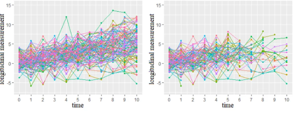
4.1 Longitudinal measurements generated from Algo-rithm 3 for 100 individuals. . . 53 4.2 Frequency of dropout times and censored times from
simulated data in Figure 4.1-(b). . . 54 4.3 Observations of the individuals from the initial study,
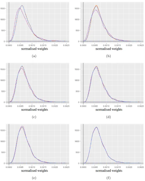
eleven observations for a new individual, and four new observations for an individual originally in the study. . . 59 4.4 Distribution of the approximate normalised weights
obtained by Monte Carlo and quasi-Monte Carlo in-tegration methods. . . 62 5.1 Cumulative incidence function for alive discharge
from the ICU or death in the ICU. . . 72 5.2 SOFA and SOFA∗ longitudinal measurements for
pa-tients who discharged alive, died, and were adminis-tratively censored. . . 74 5.3 Individual estimation of the dynamic cumulative
in-cidences foralive discharge from the ICU andeath in the ICU for patient 12 and 131 in the study. . . 86
List of Tables
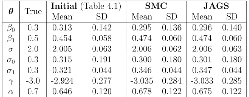
4.1 Posterior summaries of the parameters and hyperpa-rameters of the joint model (4.2) using JAGS. . . 56 4.2 Posterior summaries of the parameters and
hyperpa-rameters of the longitudinal model (4.5) using JAGS. . 57 4.3 Marginal posterior expectation and standard
devia-tion of θ before and after incorporating all new ob-servations. . . 66 5.1 Posterior summaries of the parameters and
hyperpa-rameters of the joint model (5.1) and (5.3) using JAGS. 78 5.2 Marginal posterior expectation and standard
devia-tion of θ before and after incorporating all new ob-servations. . . 85
Notation
Symbols and nomenclatures
∝ Proportionality.
∼ Has distribution.
∈ Is an element of.
lim Limit.
Z Set of integer numbers.
< Set of real numbers.
N Number of individuals.
i Index for individuals.
v Index for competitive events.
k Index for particles.
t Time in process.
∆t Incremental time.
C Censoring time.
T∗ Time until the event of interest.
T Observed event time, min(T∗, C).
δ Event indicator.
n Number of longitudinal observations.
g Number of new longitudinal observations.
tj jth observed longitudinal time.
yj Longitudinal observation at timetj.
t1:n Firstnobserved longitudinal times.
D,D1,D2 Sets of observed data.
Dgi Set of theg new observed data of the individuali.
j Term error at timetj.
1:n Term errors at timest1:n.
σ2 Longitudinal variance error term.
β’s,γ’s Fixed effects parameters. b,b0,b1 Random effects.
σ2
0,σ12 Random effects variances term.
λ’s,ν’s Parameters of the baseline hazard function.
α’s Association parameters between processes. θ Vector of parameters and hyperparameters.
K Size of the marginal posterior samples ofθ.
KT Threshold (degeneracy criterion).
M Number of replicated particles (resampling step).
L Number of integration nodes (Monte Carlo approach).
Q Number of points (Gauss-Legendre quadrature rule).
u Simulated nodes or points.
θ(k) Components of thekth particle.
e
w(k) kth unnormalised incremental importance weight.
w(k) kth normalised incremental importance weight.
f(D |b,θ) Likelihood function of (b,θ).
f(D |θ) Marginal likelihood function ofθ. ˆ
f(D |θ) Approximation of the marginal likelihood function ofθ.
π(θ) Prior distribution ofθ.
m(D) Normalising constant.
π(b,θ| D) Posterior distribution of (b,θ).
π(b| D) Marginal posterior distribution ofb.
π(θ| D) Marginal posterior distribution ofθ.
π(b| D,θ) Conditional posterior distribution ofbgivenθ.
y Longitudinal process.
s Time-to-event process.
x Vector of covariates.
f(y,s,b,θ |x) Full joint probability distribution of (y,s,b,θ) givenx.
f(y,s|b,θ,x) Conditional joint distribution of (y,s) givenb,θ, andx.
f(b|θ,x) Distribution ofbgivenθ andx.
f(y| ·) Marginal distribution ofy.
f(s| ·) Marginal distribution ofs.
p(t) Probability for the Bernoulli process at timet.
h(t| ·) Hazard function at timet.
h0(t) Baseline hazard function at timet.
S(t| ·) Survival function at timet.
F(t| ·) Distribution function at timet.
H(t| ·) Cumulative hazard function at timet.
P(·) Probability.
P(θ >0| D) Posterior probability that parameterθis positive.
P(·) Generic probability distribution.
Operators and functions
A> Transpose of matrix (or vector)A.
F−1(·) Inverse of the functionF(·).
z(·) Link function.
η(·) Linear predictor.
E(X) Expectation of the random variableX. Var(X) Variance of the random variableX. min(a, b) Minimum betweenaand b.
ka1:nk2 Euclidean distance: Pnj=1a 2
j.
x→a xconverges to a.
I(C(x)) Indicator function of the setC (1 ifx∈C, 0 otherwise). log(·) Logarithmic function of basee(ln).
exp(·) Exponential function. Γ(·) Gamma function.
diag(a) Square diagonal matrix withaon the main diagonal.
Usual probability distributions
Bernoulli B(p). Gamma G(α, β). Normal N(µ, σ2). Uniform U(a, b). Weibull W(λ, ν).
Abbreviations
AI Asynchronies index.
CIF Cumulative incidence function. ESS Effective sample size.
ICU Intensive care units.
IBIS Iterated batch importance sampling. JAGS Just Another Gibbs Sampler. SOFA∗ Logarithm of (SOFA+1).
MAR Missing at random.
MC Monte Carlo.
MCAR Missing completely at random. MCMC Markov chain Monte Carlo. MNAR Missing not at random. MV Mechanical ventilation.
QMC Quasi-Monte Carlo.
SD Standard deviation.
SOFA Sequential organ failure assessment. SMC Sequential Monte Carlo.
Chapter 1
Background
The motivation of this thesis follows the current trend in medi-cal practices towards personalised medicine1 (Sharratt, 2015). This term is well defined according to the Personalized Medicine Coali-tion2 as
[Personalised medicine is] an evolving field in which physicians use diagnostic tests to determine which med-ical treatments will work best for each patient. By com-bining the data from those tests with an individual’s medical history, circumstances and values, health care providers can develop targeted treatment and preven-tion plans.
More briefly, following the National Academy of Sciences3
1Also referred to as precision medicine, stratified medicine, individualised
medicine, or P4 medicine.
2PMC:
http://www.personalizedmedicinecoalition.org
3NAS:
2
[Personalised medicine is] the use of genomic, epige-nomic, exposure and other data to define individual pat-terns of disease, potentially leading to better individual treatment.
Personalised medicine may be seen as the tailoring of medical treat-ments to specific individuals as well as the needs and preferences of a patient during all stages of care, including prevention, diagno-sis, treatment, and follow-up (Food and Administration, 2014). In contrast, we have the population medicine which can be understood as the study of a group of individuals in order to extrapolate the findings to the general population (Mega et al., 2014).
The practice of personalised medicine is considered as the new era of medicine. However, this idea is not new and has been practiced by clinicians ever since the dawn of western medicine over 2000 years ago (Murugan, 2015). Indeed, the famous Greek physician Hip-pocrates of Cos (460 B.C. - 370 B.C.) is considered the precursor of personalised medicine as well as the “father of western medicine”. At that time, he already glimpsed about the “individuality” of dis-eases and the importance of the prescription of different medicines to different patients (Schiefsky, 2005).
Statistical science is an essential part of medical research that has been used in modern medicine, drug development, and epidemiol-ogy (Chakra-Borty and Moodie, 2013; Lu et al., 2015). In recent decades, the statistical methods have greatly contributed to the comprehension of the epidemiology of various diseases as well as
to the connection between them and biomarkers4 and/or symptoms (Cho et al., 2012; Collette et al., 2012; Zhao and Zeng, 2013; Jain, 2015). Within the diversity of methodologies that can be applied in this field, some of them may be highlighted given their importance in approaching personalised medicine. These are the models for lon-gitudinal data (Bandyopadhyayet al., 2011; Verbeke et al., 2014) or time-to-event data (Bewicket al., 2004) or models for jointly study-ing both type of data (De Gruttola and Tu, 1994; Tsiatiset al., 1995; Faucett and Thomas, 1996; Wulfsohn and Tsiatis, 1997; Henderson
et al., 2000; Tsiatis and Davidian, 2004; Ye et al., 2008; Rizopoulos, 2012b).
The next two sections of this chapter are designed to describe, in a separate form, the key ideas behind longitudinal and time-to-event data. Then, in Section 1.3 we will discuss the importance of a joint analysis of both types of data. Finally, in Section 1.4 we will introduce the Bayesian perspective for this joint modelling as well as the need for sequential update methodologies.
1.1
Longitudinal data
Longitudinal data5 are a particular type of correlated data where a given set of variables are repeatedly measured over time in the same
4A biomarker is a characteristic that is objectively measured and
evalu-ated as an indicator of a normal biologic process, disease process, or biological response to a therapeutic intervention. Biomarkers can be used to reduce un-certainty and guide clinical care.
4 1.1. Longitudinal data
sampling unit. Longitudinal data analysis confronts with cross-sectional studies in which a single observation is measured for each individual. Longitudinal approaches can work with different corre-lation structures, such as serial correcorre-lation, shared random effects, transition (Markov) models, latent classes, clustering, etc. (Verbeke and Molenberghs, 2000).
One of the most important aspects of this type of data is the nat-ural hierarchical structure of the variability with different levels of interest. For instance, we can consider as a first level effect a group mean response for all individuals over time, while a second level cap-tures individual-specific feacap-tures using, for instance, random effects (Gelman and Hill, 2006). The incorporation of individual sources of variability provides the ability to predict the trajectory of indi-vidual responses and understand how do them change with respect to the general mean in the population of interest (Laird and Ware, 1982; Verbeke et al., 2001). Furthermore, there is also the possibil-ity for describing how the mean response changes in the population of interest. All these characteristics make the longitudinal models extremely convenient in many research fields, e.g. medicine, pub-lic health, education, business, economics, psychology, and biology (Weiss, 2005).
Missing data6 can greatly affect the longitudinal analysis depending on the processes causing them. Missing data can be classified into three types: missing completely at random (MCAR); missing at ran-dom (MAR); or missing not at ranran-dom (MNAR) (Little and Rubin,
2002). The last case, MNAR, is the most important in the longi-tudinal studies, since it can be hiding some latent process which, if ignored, can produce biased estimates and predictions. This is why they are also known as nonignorable missing data (for reviews, see Molenberghs and Kenward, 2007). Time-to-event models, described in the next section, can be useful for modelling the process that gen-erates the MNAR data, and hence avoiding the bias in the results (Ibrahim and Molenberghs, 2009).
1.2
Time-to-event data
We consider time-to-event data whenever we are interested in the time until an event of interest occurs. As pointed out by Col-lett (2003), this type of data arises in a great number of applied fields, such as medicine, public health, epidemiology, biology, envi-ronmental sciences, engineering, economics, actuarial sciences, man-agement, demography, and social sciences
The nomenclature time-to-event analysis may change according to the area of research, e.g. it is usually referred to assurvival analysis in medicine and biology (Box-Steffensmeier and Jones, 2004; Klein-baum and Klein, 2012) and reliability analysis in engineering and industrial studies (Jewell et al., 1996; Couallier et al., 2013). In numerous medical studies, survival probabilities are of primary interest, since their estimates for a specific patient can rule de-cision making involving specific interventions (Rizopoulos, 2011).
6 1.2. Time-to-event data
Commonly, the standard statistical procedures are not amenable for time-to-event data due to its particular features: the response variable is positively skewed and some observations are typically in-complete in the sense that some factor (external to the study or intentionally planned) prevents the event of interest from being ob-served (Lee and Wang, 2013). Some situations that illustrate those types of behaviour are: the study ends without the patient having experienced the event, an intervening event that occurs prohibit-ing further observation on the patient, the patient can be missprohibit-ing at some time point, or even the patient withdraws from the study (Merrill, 2015).
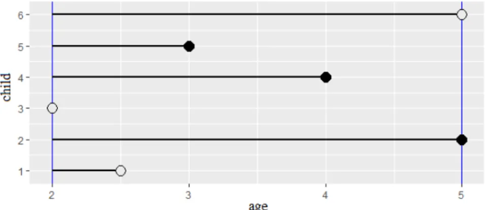
Depending on the reason why the event has not been observed we will refer to censoring or truncation. To illustrate the differences between them, we consider a toy example which focuses on children in the kindergarten, from 2 to 5 years-old, where our event of interest is the age at which these children learn to write their own name. Let us suppose that children are annually evaluated to know if they have learnt to write their name. Evaluation for children aged 2 and 5 are also included in the analysis. In this example, we will consider only six children randomly chosen from a hypothetical population. Let us assume that child 1 moves to a different school at age 2.5 without having experienced the event of interest. In the initial ex-amination (at 2 years-old), it was verified that child 3 already knew how to write his/her own name. Children 2, 4, and 5 experienced the event of interest within the study interval. In addition, the last evaluation (at 5 years-old) revealed that the child 6 had not yet
learned to write his/her own name. Figure 1.1 shows the data from this example.
Figure 1.1: Age, in years, at which each child in the study learns to write their own name. Blue solid vertical lines indicate the learning period in the kindergarten. Solid circles represents
observed times and open circles censored times.
We will refer to censoring data whenever the time of the event is only partially known (Leunget al., 1997). This is, we know that it is larger (right censoring), smaller (left censoring), or within an inter-val (interval censoring) of observed times (Klein and Moeschberger, 2003). In our example, time for child 1 is right-censored because he/she left the study without having experienced the event of inter-est. Time for child 6 is also right-censored, but now because he/she has not experienced the event when the study ends. Time for child 3 is left-censored, since he/she knew how to write his/her name at the time of his/her entrance in the study. Times for children 2, 4 and 5 are interval-censored because we only know that these children had learnt to write their own name in a time between two consecutive annual evaluations.
8 1.2. Time-to-event data
Truncation is a variant of censoring, where the incomplete nature of the observations happens because of a systematic selection process inherent to the study design (Andersen et al., 1993). In practice, truncation imposes restrictions in the limits of the period of study and only individuals with observed event time within them are con-sidered in the analysis (Klein and Moeschberger, 2003). Hence, we can basically limit the period of study in three ways: only an upper limit (right truncation), only a lower limit (left truncation), or an interval limit (interval truncation).
Going back to our toy example, let us imagine that two 3-years-old children enter the study and it is verified through the learning examination that one of them already knows how to write his/her own name. In this case, the child who passed the exam has a right truncation time, since he/she experienced the event of interest be-fore entering the study. On the other hand, we already know that the other new child is not able to write his/her own name until 3 years-old, so this child has a left truncation time (or delayed entry time). Now let us suppose that child 1 at age 4 is transferred back to our kindergarten. This child took the learning examination and was approved. In this case, child 1 has a interval truncation time, since we know he/she experienced the event of interest after 2 and before 4 years-old. It is important to remark that truncated data leads to conditional probabilities/estimations, since we know that the event time is limited superiorly and/or inferiorly by truncations. Time-to-event analysis also allows the inclusion of covariates to im-prove the probabilistic modelling of the occurrence of the event of
interest. A great challenge in this sense is the incorporation of time-varying covariates, mainly those of endogenous (or internal) nature in which traditional approaches are not applicable (Molen-berghs et al., 2014). This is due to the fact that the occurrence of the event of interest at a time point affects (or prevents from being observed) the values of these covariates (Rizopoulos, 2012b). Typically, biomarkers directly related to the risk of the event of in-terest are endogenous time-varying covariates (Kalbfleisch and Pren-tice, 2002). They usually have a longitudinal nature that can be incorporated into the time-to-event analysis using joint models.
1.3
Joint models for longitudinal and
time-to-event data
Joint modelling has recently attracted great attention to the sta-tistical community, especially in the area of biostasta-tistical research (Rizopouloset al., 2010). Yu et al.(2004) discuss some of the main objectives of this type of models. Among them we highlight
• The study of a longitudinal response variable and its associ-ation with baseline covariates, treatments, and specific char-acteristics of the individuals of the population sample avoid-ing the possible bias due to MNAR data, which are modelled through a time-to-event process (see Section 1.1);
• Characterising the risk of an event with regard to a longitu-dinal variable (endogenous covariate) or to the time when a
10 1.3. Joint models for longitudinal and time-to-event data
longitudinal variable was observed (surrogate endpoint) (see Section 1.2).
In both cases, the final interest is usually to make estimation and/or prediction of longitudinal individual or population trajec-tories and/or relevant outcomes associated to the occurrence of the event of interest. Moreover, we could consider a general approach that takes both objectives into account.
Currently, many studies combine the power of the junction of both types of data, since a separate analysis of the longitudinal and time-to-event data may lead to inefficient or biased results (Yu et al., 2008; Ibrahim et al., 2010; Wu et al., 2012).
Research literature for joint models uses the frequentist (or classi-cal) and Bayesian approaches to estimate and predict information of interest (for interesting reviews up to date, see Tsiatis and Da-vidian, 2004; Neuhaus et al., 2009). In particular, this modelling is relatively new for the Bayesian approach and so it is devoid of some more in-depth research topics, such as sensitivity analysis to the elic-itation of prior distributions, sequential update, model validation, and model selection.
A key feature in real studies with this type of models is the dynamic nature in which data become available. This is clear in biomedical studies where data usually come from individual follow-ups over time. Thus, when new information of a given patient is collected, physicians are interested in updating the relevant estimated and/or predicted outcomes.
Dynamic inference is an inherent difficulty within the frequentist joint modelling, since the number and timing of interim analyses directly affect some frequentist properties (Lee and Chu, 2012). Hence, the current literature has proposed two paths: (i) taking asymptotic assumptions in order to only update the subject-specific effects (Rizopoulos, 2011; Mauguen et al., 2013; Andrinopoulou
et al., 2015a; Barrett and Su, 2017) or (ii) moving towards a Bayes-ian approach (Yu et al., 2008; Proust-Lima and Taylor, 2009; Ri-zopoulos et al., 2014; Andrinopoulou et al., 2015b).
In the next section, we will introduce some advantages of the Bayes-ian approach as well as its sequential learning for dynamic inference.
1.4
A Bayesian view of joint models
Bayesian statistics is founded upon the premise that all unknown quantities (or sources of uncertainty) should be expressed and mea-sured by probability distributions (Bernardo and Smith, 1994). In other words, it associates probability measures to any random quan-tity, parameter, event, hypothesis, model, etc. (for reviews, see Loredo, 1990, 1992).
In the case of joint models for longitudinal and time-to-event data, the Bayesian perspective makes it possible to incorporate prior in-formation to the study, thus improving and enhancing estimation and prediction of any outcome of interest (Guo and Carlin, 2004). In particular, we can also estimate and predict characteristics of the
12 1.4. A Bayesian view of joint models
longitudinal variable for individuals in the current sample or even for new individuals, from the same study population, that could en-ter to the study. However, the more relevant Bayesian issues deal with the direct estimation of the survival function, the prediction of survival times, or the computation of other posterior distributions for relevant probabilities or rates. The frequentist approach for this type of models is extremely complex because the probabilistic char-acteristics of the relevant estimators are practically impossible to compute (Ibrahim et al., 2001).
The Bayesian approach of joint models is gaining considerable atten-tion from the scientific community, mainly in the medical sciences (Brown and Ibrahim, 2003; Ibrahim et al., 2004; Hu et al., 2009; Huang et al., 2010, 2011; Zhu et al., 2012; Baghfalaki et al., 2014; Huanget al., 2014; Armero et al., 2016a,b; Martinset al., 2016, and references therein). One of the main factors for the proliferation of the Bayesian approach for joint models is its conceptual simplicity (Gould et al., 2014). Moreover, the improvement of Bayesian com-putational methods, the increase of the processing capacity, and the development of Bayesian statistical software and packages has con-tributed to the use of multilevel7 models, which can be considered as a natural framework for joint models.
Another motivation in favour of the Bayesian methodology is our interest in dynamic inference. The reason is simple and concep-tual. The posterior distribution is the most relevant element of the
7Other related names: hierarchical linear models, nested models, random
parameter models, random coefficient, random-effects models, mixed models, or split-plot designs.
Bayesian approach, because besides being the probabilistic represen-tation of the total knowledge about the parameters after the data and any other relevant information have been considered (Glickman and van Dyk, 2007), it is also the starting point of all relevant infer-ences. The posterior distribution combines the likelihood function, interpreted as the information about the parameters contained in the data, and the prior distribution, which represents prior expert knowledge about the parameters. Bayesian learning consists of the sequential application of Bayes’ theorem for updating the posterior distribution with information provided by new experimental data (Barber, 2012).
Nowadays, most of the packages for joint models8 are implemented from a frequentist perspective and do not incorporate mechanisms of dynamic inference. The only package that uses a Bayesian per-spective isJMbayes, which, despite it does not make fully Bayesian dynamic inference, proposes a mechanism based on asymptotic the-ory for dynamic prediction (for more details, see Rizopoulos, 2011). Bayesian inference within joint modelling can also be done using general Bayesian software/packages, such as the BUGS language (Win/OpenBUGS (Lunn et al., 2000) and JAGS (Plummer, 2003)), Stan (Hoffman and Gelman, 2014), and INLA (Rue et al., 2009), but so far none of them incorporates dynamical procedures.
8In
R: lcmm (Proust-Lima et al., 2010), JM (Rizopoulos, 2010), joineR
(Philipsonet al., 2012),JMbayes(Rizopoulos, 2012a),JMdesign(Corneaet al., 2014),JSM(Xuet al., 2016),joint.Cox(Emura, 2016), andfrailtypack
(Ron-deauet al., 2017). InSAS: JMFitmacro (Zhang et al., 2016). InSTATA:stjm
14 1.5. Outline
Our main objective in this thesis is to propose an entirely inferen-tial and predictive Bayesian analysis for joint models by means of a dynamic update methodology based on sequential Monte Carlo9 methods (Capp´eet al., 2007). Therefore, our challenge is to combine the flexibility of the Bayesian approach for joint models of longitu-dinal and time-to-event data with a learning procedure constructed through sequential methods.
As far as we know this thesis is the first proposal that fully integrates the Bayesian joint models with sequential Monte Carlo methods.
1.5
Outline
After this introductory chapter aiming to briefly introduce Bayesian joint modelling for longitudinal and time-to-event data and motivate the need of sequential Monte Carlo methods to achieve dynamic es-timation and prediction in such models, the rest of this thesis is structured as follows. Chapter 2 reviews the Bayesian paradigm and presents sequential Monte Carlo methods. Chapter 3 contains the special features of sequential Monte Carlo methods tailored to the framework of joint modelling for longitudinal and time-to-event data. This chapter may be regarded as the core of the thesis. Chap-ters 4 and 5 illustrate our proposals. In particular, Chapter 4 pro-vides the development of a simulation mechanism for generate data from a joint model with longitudinal objective and nonignorable
9Other related names: particle filtering, Monte Carlo filter, survival of the
fittest, sequential imputations, condensation, bootstrap filter, or sequential im-portance resampling.
dropout. From a generated data set with this mechanism, we ex-emplify the benefits of a joint analysis for longitudinal data with informative dropout. Still in this chapter, we explore in detail the use of our proposal of sequential updating for a shared-parameter joint model. Chapter 5 explores the dynamic posterior estimation and prediction for a random-effects joint model constructed in terms of a longitudinal linear mixed submodel and a survival competing risks submodel. This is a joint model for a real study devoted to the analysis of the association between a severity marker and the events alive discharge and death for patients receiving mechanical ventilation in intensive care units. Chapter 6 presents the main con-clusions and contributions of the thesis as well as a brief discussion about future research on the subject. We have also included three appendices. Appendix A contains the JAGS codes of the simulated model implemented in Chapters 4 and 5. Appendix B presents a list of the common probability distributions and their basic properties. Appendix C provides a posterior summary of the results obtained in simulated scenarios based on different parameter configurations. This thesis ends with a final section devoted to Bibliography.
Chapter 2
Sequential learning
Learning theory is broadly a framework for machine learning1 that comes from the fields of statistics and functional analysis (Mohri
et al., 2012). In essence, statistical learning refers to a set of ap-proaches for inferring and predicting from available data (Hastie
et al., 2009; James et al., 2013). In addition, it also plays an im-portant role for sequential settings, such as classification problems (Syed et al., 2009).
In particular, sequential learning can be defined in statistical terms as the mechanism to improve estimation and prediction after observ-ing new data (Dietterich, 2002). The way of processobserv-ing knowledge in the sequential learning framework is similar to the human ability to learn from previous experiences (Clegg et al., 1998).
1Machine learning is a set of rules and procedures, which allows computers to
act and make decisions based on data rather than being explicitly programmed to perform a certain task.
18
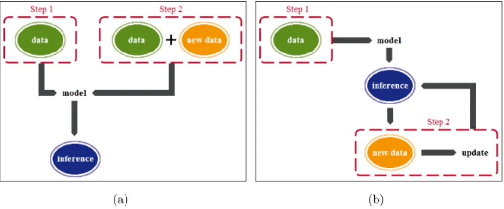
In the context of statistical inference, Figure 2.1-(a) shows a generic scheme of a non-sequential inferential process from a general model.
(a) (b)
Figure 2.1: Non-sequential (a) and sequential (b) procedures.
In this illustration, Step 1 works with data and Step 2 with the previous data plus new data. Note that inStep 2 we proceed as if all the available data were new, despite part of them were already used inStep 1. Figure 2.1-(b), instead, uses only new data to update the inferential process, without the necessity of a “complete oblivion” of the results previously obtained. The idea of sequential learning is to avoid the rework illustrated in Figure 2.1-(a) maintaining the accuracy of the results.
As pointed out in the introductory chapter, our objective is to de-velop a full Bayesian learning process for making dynamic inference and prediction in joint models for longitudinal and time-to-event data. Hence, in the following sections we will introduce the basis of the Bayesian approach as well as Bayesian sequential methods that will be adapted to the context of the joint models encompassed in this thesis.
2.1
Bayesian approach
As briefly discussed in Section 1.4, Bayesian inference contains two key ingredients. The first element is the likelihood function of the parametric vector θ, f(D | θ), which summarises the information available in the dataD aboutθ. The second ingredientπ(θ), called
prior distribution of θ, is a probability distribution that contains all the available prior expert knowledge about θ. From these two terms, the inferential process should naturally be summarised by the probability distribution of θ after observing the value of D. This distribution, π(θ | D), is known as the posterior distribution of θ
and it is obtained according to the Bayes’ rule:
π(θ | D) = f(D |θ)π(θ)
m(D) ∝f(D |θ)π(θ), (2.1) where m(D) = R
f(D | θ)π(θ) dθ is the normalising constant, also called model evidence of the data D (Robert, 2007). This constant that makes the posterior distributionπ(θ| D) integrate to one. The basis of the Bayesian methodology is simple and intuitive. It combines different sources of information that can be associated to the way in which the human brain works, always learning from past experiences. The Bayesian approach offers comprehensive and powerful tools to complex model estimation and prediction as well as all relevant quantities of interest derived from the inferential process (Carlin et al., 2001; Gilks et al., 1993).
One of the main advantages of the Bayesian methodology is that, independently of the complexity of the model, it always follows the
20 2.1. Bayesian approach
same structure based on the posterior distribution ofθ in (2.1). In addition, the prior distribution of θ may incorporate prior knowl-edge, often based on expert or information accumulated from pre-vious studies, which in many cases makes posterior estimates more accurate (Bayarri and Berger, 2004). Furthermore, Bayesian per-spective does not need to assume asymptotic assumptions, as is common in the frequentist paradigm (Ibrahim et al., 2001).
Even with all these advantages, the beginning of the Bayesian methodology was frustrating because, despite being theoretically appealing, it was almost always inapplicable in practice. The big challenge was (and in some sense still is) to handle with non-standard probability densities, especially in high-dimensional prob-lems (Robert, 2014). In particular, the main difficulty was to calcu-late the normalising constant m(D) and to obtain a sample of the posterior distribution ofθ, π(θ | D) (Robert and Casella, 2004). After a long period of dormancy (McGrayne, 2011), the Bayesian perspective resurfaced in the early 90s due, mainly, to the evolu-tion of technology (computers with more processing capacity and more affordable prices) and the development of stochastic integra-tion methodology, especially Markov chain Monte Carlo (MCMC) approaches, such as Gibbs sampling and Metropolis-Hastings algo-rithms (Geman and Geman, 1984; Gelfand and Smith, 1990; Carlin and Chib, 1995; Gelfand, 2000; Gamerman and Lopes, 2006). These advances entailed a substantial increase of the number of publica-tions involving Bayesian methods in many scientific areas (Robert and Casella, 2011). More recently, other Bayesian procedures based
on analytical approximations of the posterior distribution have also appeared, such as variational Bayesian methods (Beal, 2003) and integrated nested Laplace approximations (Rue et al., 2009). How-ever, for the inference in many contexts, such as most part of join models, we are still restricted to the use of MCMC methods. Sequential inference is one of the more important scenarios where Bayesian methodology has gained very much popularity (Creal, 2012). The reason is that the Bayesian inference provides a nat-ural, elegant, and unified approach to sequential learning (Freitas
et al., 1999).
For an illustration of Bayesian reasoning in sequential learning, sup-pose a given generic model with parametric vector θ for which we want to make inference from only a set of available observationsD1. The posterior distribution ofθ,π(θ| D1), is computed by applying the Bayes’ rule from the likelihood function ofθ,f(D1 |θ), and the prior distribution of θ, π(θ), as shown in (2.1). Then, in a second step, we observe a new set of observationsD2 and we want to update our knowledge about θ obtaining a “new” posterior distribution of
θ, π(θ | D1,D2). This sequential procedure can be summarised by equations (2.2) and (2.3) as follows:
Step 1: π(θ| D1)∝f(D1 |θ)π(θ). (2.2)
Step 2: π(θ| D1,D2)∝f(D2 | D1,θ)π(θ| D1). (2.3) However, it is quite common that the “first” posterior distribution of θ, π(θ | D1), has not an analytical expression, i.e., we only have an approximated sample of it thus making the sequential inferential
22 2.2. Sequential Monte Carlo methods
process “not-so-easy” in practice. In such cases, equivalent infer-ences can be obtained through a Bayesian inferential process based on the set that integrates the old and new data:
π(θ | D1,D2)∝f(D1,D2 |θ)π(θ). (2.4) Nevertheless, this procedure is not always a real alternative because it may be computationally very costly in terms of both, time and resources.
To circumvent the problem thatπ(θ | D1) is analytically intractable, a great number of sophisticated techniques have been proposed in recent years, in particular sequential Monte Carlo methods. These are a general class of numerical methods, which provide samples from a target distribution (let’s say the posterior distribution) based on weights calculated from importance sampling and resampling mechanisms (Kantas et al., 2009; Gao and Zhang, 2012).
In the next section, we will introduce sequential Monte Carlo meth-ods and their main peculiarities.
2.2
Sequential Monte Carlo methods
Among the numerous sequential Bayesian learning approaches, the most efficient methods for inference are the sequential Monte Carlo (SMC) methods (Lopes and Tsay, 2011). SMC methods are a set of simulation-based procedures which provide an appropriate and
clever approach to sequentially update complex posterior distribu-tions. These methods are flexible, applicable to very general set-tings, and their implementations are intuitive and allow parallel processing (Doucet et al., 2001).
In general, SMC methods are employed in a plethora of applica-tions involving artificial intelligence, bioinformatics, computational physics, computational science, economics and mathematical fi-nance, engineering and robotics, machine learning, molecular chem-istry, pharmacokinetic, phylogenetics, signal and image process-ing, simultaneous localization and mappprocess-ing, target trackprocess-ing, among other fields (Jouin et al., 2016). In all these frameworks, the pa-rameters and/or states2 of interest are commonly associated with time or some similar dependent structure, more specifically known as state-space (or hidden Markov) models (Crisan and Rozovskii, 2011).
SMC methods approximate the target distribution using a set of simulated samples (particles) and their respective weights. They adopt a sequential strategy for updating that distribution incorpo-rating the information provided by new data (Bonawitzet al., 2014). The performance of these methods depends on the number of parti-cles, in which a very large number indicates a better representation of the target distribution.
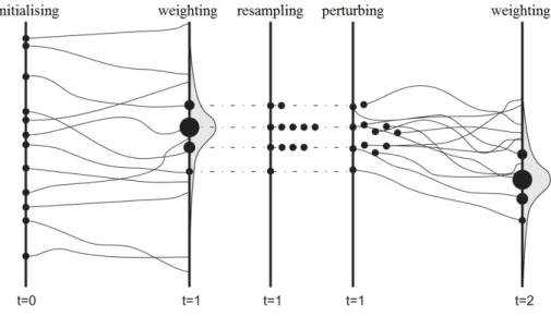
Figure 2.2 illustrates the step by step of the general SMC scheme with 12 particles (circles). In order to facilitate the understanding
2Unobserved (or hidden) process that connects the dynamic nature of the
response variable with a conditional model for the observed process given the state(s).
24 2.2. Sequential Monte Carlo methods
Figure 2.2: Sequential Monte Carlo scheme. (Source: Montzka et al., 2012)
of the graphic, let us imagine that these particles synthesise the distribution of a parameter θ that needs to be updated. The size of each circle in a given step is related to the weight of the spe-cific particle. Att = 0 the particles are distributed over an interval (vertical axis) that can be interpreted as the domain of the values where the parameter θ is defined, with all its particles having equal weights. Att= 1 we have the first observation(s) and the sequential update procedure is initialised. The first step at t = 1 (weighting) consists in obtaining the weights of the particles according to the information provided by the new observations. In the second step at
t= 1 (resampling), the set of particles is resampled with probabili-ties proportional to their weights which are then reset to be equally likely. In the third step at t = 1 (perturbing3) the particles are
3Perturbing step does not exist in some sequential methods, e.g. sequential
moved to avoid their accumulation in a few values. The next time pointt = 2 represents access to new observed data and the restart-ing of the update procedure from the weighting step. Although it does not appear explicitly in Figure 2.2, before performing the re-sampling andperturbing steps, the “good quality” (efficiency) of the new particles should be checked (Arulampalam et al., 2002). This is done according to some degeneracy criterion. The problem of de-generacy occurs when only a few particles representing the target distribution have significant weights. Further down we will display the most standard way of measuring this degeneracy.
As previously mentioned, this class of sequential methods was (and in some sense still is) primarily developed for state-space models, where parameters/states are time dependent. This is not the situa-tion in joint models4 where all parameters and/or hyperparameters are static in the sense that they do not change in time. For this reason we focus on SMC methods for models of static parameters (also known as static models) and we are thus faced to the pro-posal by Chopin (2002) and other works with the same background (Ridgeway and Madigan, 2003; Balakrishnan and Madigan, 2006; Del Moral et al., 2006; Capp´e et al., 2008; Sch¨afer and Chopin, 2013; Fearnhead and Taylor, 2013; Chopin et al., 2013). The algo-rithm proposed in Chopin (2002), called iterated batch importance sampling (IBIS), aims to approximate a target distribution of static parameters and hyperparameters, e.g. π(θ | D1,D2) in (2.3), using
4Technically, we could employ non-static joint models, but this thesis only
26 2.2. Sequential Monte Carlo methods
a sample of a “prior distribution”, e.g. π(θ | D1) in (2.2), through the scheme presented in Figure 2.2.
Our starting point is an approximate random sample of sizeK from the posterior distribution of θ, π(θ | D1), obtained through a nu-merical Bayesian procedure5. After this initial stage and with new data, D2, available, the update process using the IBIS algorithm has four steps: initialising, weighting, resampling, and moving (or
perturbing) (see Figure 2.2).
The first step (initialising) is used to generate a particle system
θ(k), w(k), whereθ(k) is drawn from the “first” posterior distribu-tion of θ, π(θ | D1), and the weight w(k) of each sampled particle
θ(k) is equal to 1/K, for k = 1, . . . , K. This first step is performed only once, while the next ones are iterative as more data becomes available.
Theweighting step is based on importance sampling and resampling techniques (Rubin, 1987, 1988). Basically, they rely on an impor-tance distribution to calculate the “changes” in the target distribu-tion, e.g. π(θ | D1,D2), through (incremental importance) weights. The choice of an appropriate importance distribution is the key for an efficient update to be sequentially performed. In short, it must be a good approximation of the target distribution. So provided that new data D2 should not alter much the inference about the param-eters obtained withD1, π(θ | D1) andπ(θ | D1,D2) are likely to be similar. Hence, we define the importance distribution as π(θ | D1) and then update the unnormalised weights we(k), for k = 1, . . . , K,
based on the likelihood function of the new data: e w(k) ∝ π θ (k)| D 1,D2 π(θ(k) | D 1) ∝ f D1,D2 |θ (k) π θ(k) f(D1 |θ(k))π(θ(k)) = f D2 | D1,θ (k) f D1 |θ(k) f(D1 |θ(k)) =f D2 | D1,θ(k) . (2.5) Then the weightswe(k), k= 1, . . . , K, are normalised to sum to one. Next, we have a resampling (or selection) step. The principle of resampling is simple: the particles with low normalised importance weights are discarded with a high probability, while those that re-main are replicated. Figure 2.3 illustrates a generic resampling scheme.
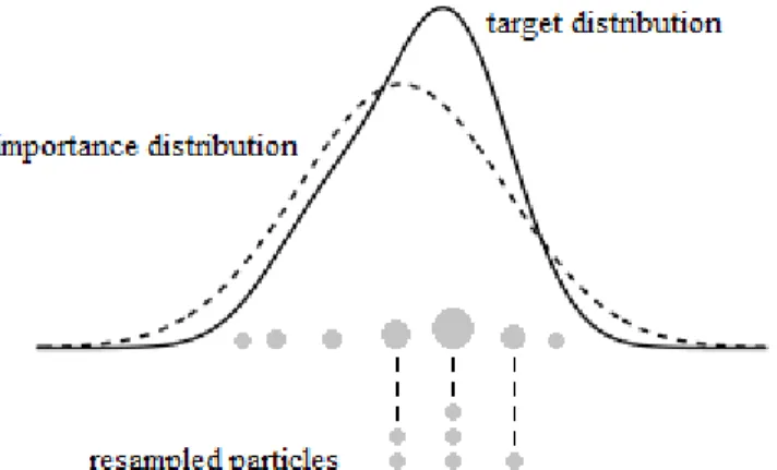
Figure 2.3: Graphical illustration of theresampling step. (Source: modified from Capp´e et al., 2005)
Initially (top of the Figure 2.3), we have the target posterior dis-tribution π(θ| D1,D2) (solid line), the importance distribution π(θ | D1) (dashed line), the particles (circles), and the weights (size of the circle) as inweighting step. Then (bottom of the Figure 2.3),
28 2.2. Sequential Monte Carlo methods
the particles are resampled taking into account their normalised im-portance weights andM particles are selected with weights reset to 1/M (in the Figure 2.3, K = 7 and M = 6).
The resampling step maintains (the majority of) the particles in regions of high probability mass then culminating with the reduction of the number of particles to represent the target distribution, and diminishing consequently the computational effort (Doucet et al., 2000; Del Moral et al., 2012).
It is important to remark that the resampling step increases the Monte Carlo variance (Chopin, 2004), but it does not change the expected value of the target distribution, i.e., the estimators are kept unbiased (Petris et al., 2009). In addition, resampling eliminates the accumulation of errors over time and provides better stability for predictive distributions (Douc et al., 2014). These concepts are precisely characterised by existing convergence results (Doucet and Johansen, 2011).
Manyresampling procedures that keep under control the increasing Monte Carlo variance while preserving the unbiasedness property have been proposed (Douc and Capp´e, 2005; Hol et al., 2006). The most popular of them are multinomial resampling (Gordon et al., 1993), residual (or remainder) resampling (Whitley, 1994; Liu and Chen, 1998), stratified resampling (Kitagawa, 1996), and systematic resampling (Whitley, 1994; Carpenter et al., 1999). Since this the-sis does not focus on quality and/or computational complexity of resampling methods, we will only use the multinomial resampling6, which is the simplest approach.
Intuitively, replicating particles with large importance weights im-plies progressive sample impoverishment7 and high correlation be-tween the resampled particles. To avoid this problem without losing the accuracy of the results a particle rejuvenation scheme should be added (Gilks and Berzuini, 2001).
The rejuvenation of particles is achieved by means of a perturbing
step (from now on we will refer to this step as moving in order to maintain the same nomenclature used in Chopin (2002)). This step strongly reduces the degeneration of the importance weights over time. It is usually performed from an MCMC kernel with posterior distribution of θ, π(θ| D1,D2), as its stationary distri-bution (Chopin et al., 2013). The key idea is to slightly move the particles in order to maintain the diversity of the samples in the parameter space. We employ an independent Metropolis-Hastings kernel in which the proposed particles are independently generated from a normal proposal (also known as instrumental or jumping) distribution of θ based on the mean and the variance of the parti-cles according to their weights. Other options would be to use the random-walk Metropolis-Hastings or Metropolis-within-Gibbs algo-rithms (Tierney, 1994; Chib and Greenberg, 1995). This second approach is advisable when some full conditional distributions are known and easy to simulate.
6Sample M “new” particles with replacement from the set of particles
θ(1), . . . ,θ(K), where the probabilities of selection are defined by P θˇ(r) =
θ(k)=w(k) fork= 1, . . . , K andr= 1, . . . , M. UsuallyK is larger thanM.
7Also known asweight degeneracy. This phenomenon occurs when a few
par-ticles have large normalised weights while all remaining have negligible weights. It causes a deterioration in the Monte Carlo approximation.
30 2.2. Sequential Monte Carlo methods
Finally, the particle system θ(k), w(k), fork= 1, . . . , K, is replaced by the new particles and their respective weights θˇ(r), w(r)
, for
r= 1, . . . , M, and the update process is finished.
An important adaptation that Chopin (2002) incorporated into the proposal by Gilks and Berzuini (2001) is that the resampling and
moving steps are unnecessary when the weights of the particles have a small variance. This strategy significantly reduces the computa-tional time of the sequential update procedure. In other words, the “first” posterior distribution ofθ,π(θ | D1), is maintained as a good approximation for the second one, π(θ | D1,D2). However, most of the times after initialising the update process, the sample impover-ishment occurs. Hence, it is essential to establish some criterion to decide whether to continue with the same particles or perform re-sampling and moving steps. In practice, the (empirical) variability of the weights is usually evaluated through theeffective sample size
(also referenced as degeneracy criterion), which is defined as:
ESS = " K X k=1 w(k) 2# −1 = PK k=1we (k)2 PK k=1 e w(k)2 , (2.6)
and varies between 1 (when a normalised weight is equal to one) and
K (when all the weights are equal). Thus, when ESS falls below a threshold KT (typically KT =K/2), the resampling and moving
steps are triggered. Algorithm 1 shows a brief description of the SMC procedure presented in this section.
Note that the normalised weights w(k), for k = 1, . . . , K, do not appear in the calculation of incremental weight (2.5), but we have
Algorithm 1: Iterated batch importance sampling
1 Initialising:drawθ(k)∼π(θ| D1) and setw(k)←1/K,k= 1, . . . , K.
2 Weighting:from new data D2, calculate
e w(k) ←f D2 | D1,θ(k) w(k), and normalise the weightsw(k)← we
(k) PK l=1we (l), k= 1, . . . , K. if (ESS < KT) then 3 Resampling: draw θe(1), . . . ,θe(M) from θ(1), . . . ,θ(K) with probabilities proportional to the normalised weights (M ≤K). Updatew(r) ←1/M, r = 1, . . . , M.
4 Move:draw ˇθ(r) from a Metropolis-Hastings kernel of invariant
distributionπ(θ | D1,D2), r = 1, . . . , M.
Updateθ(r)←θˇ(r), r= 1, . . . , M and K ←M. end
If new data available, return toWeightingstep.
added them in the weighting step (see Algorithm 1). Recall that from the second sequential update the initialising step is no longer activated (see Figure 2.2) and so the incorporation of these weights is important, since they allow to accumulate the information from included observations in the previous update when the resampling
and moving steps were not required.
An important feature of the sequential Monte Carlo approach is that it sequentially can provide an estimate of the marginalisation constant (see (2.1)) with very little additional computation. This result is essential in model selection based on Bayes factors (Kass and Raftery, 1995). This is a very relevant and challenging issue in Statistics which is beyond the objective of this thesis. In any case,
32 2.2. Sequential Monte Carlo methods
we will briefly discuss in the next chapter the general procedure to calculate the approximate update of marginalisation constants in joint models.
Although the use of IBIS algorithm is computationally appealing by preventing us from the calculation of the posterior distribution ofθ
from scratch (considering D1 as initial data and D2 as new data), it has a major limitation in our joint models framework. This is related to the use of the so-called random effects. A statistical arti-fact that, as mentioned in Section 1.1, allow to consider individual divergences from the population behaviour. Next chapter is devoted to the introduction of some key adaptations in the IBIS approach for dealing with joint models for longitudinal and time-to-event data containing subject-specific effects.
Chapter 3
Sequential methods for
Bayesian joint models
As introduced in Chapter 1, our modelling of interest is Bayesian joint models for longitudinal and time-to-event data. The major goal of these models is the connection between the longitudinal and the time-to-event processes.
There are different types of associations between both processes (Daniels and Hogan, 2008; Fitzmaurice et al., 2008). Most of them can be modelled by some structure of unobserved latent variables and/or parameters (Sousa, 2011).
We start this chapter by introducing the main connection structures between longitudinal and time-to-event processes from a Bayesian perspective. Next, as the core of the thesis, we will extend the sequential procedures discussed in Section 2.2 to those types of joint models.
34 3.1. Bayesian joint models
3.1
Bayesian joint models
Bayesian joint models for longitudinal and time-to-event data as-sume a full joint probability distribution
f(y,s,b,θ |x) =f(y,s|b,θ,x)f(b|θ)π(θ), (3.1) whereyandsrepresent the longitudinal and the time-to-event pro-cess respectively. Random effects are denoted by b, θ represent the parameters and hyperparameters, and x is a set of covariates. Notice that each covariate in x can be related only with the lon-gitudinal or the time-to-event process or with both of them. In (3.1), f(y,s|b,θ,x) is the conditional joint distribution for the processes y and sgiven the random effects, parameters and hyper-parameters, and covariates, f(b|θ) is the conditional distribution of the random effects given θ, and π(θ) the prior distribution of the parameters and the hyperparameters of the model. The condi-tional joint probability distributionf(y,s|b,θ,x) usually depend on the assumptions about the association of both processes. The different approaches that conditionally connect the longitudinal and survival processes that we will consider in this thesis are conditional, shared-parameter, and random-effects models.
In conditional models, the conditional joint probability distribution
f(y,s|b,θ,x) in (3.1) is decomposed into the product of condi-tional and marginal distributions between longitudinal and time-to-event processes (Little, 2008). More specifically, this decomposition can be written in two opposing ways, called pattern-mixture and
selection models. Pattern-mixture models factorises the conditional joint distributionf(y,s|b,θ,x) into the product of the conditional distribution of y given s, θ, and x, and the marginal distribution of sgiven b, θ, and x.
f(y,s|b,θ,x) = f(y|s,θ,x)f(s|b,θ,x). (3.2) It is important to note that the random effects are only directly connected to the time-to-event process. Figure 3.1 illustrates the general idea for this approach.
Figure 3.1: Relationship between the longitudinal process y, time-to-event process s, and random effects b using
pattern-mixture models.
In general, this approach is used when the objective of the study is the longitudinal process y.
On the other hand, selection models assume the decomposition of the conditional joint distribution f(y,s|b,θ,x) in terms of the product of the conditional distribution of sgiven y, θ, and x, and the marginal distribution of y given b, θ, and x.
36 3.1. Bayesian joint models
In these models, the random effects are directly connected to the longitudinal process. Figure 3.2 depicts the relationship between the components of the joint process from the selection approach.
Figure 3.2: Relationship between the longitudinal process y, time-to-event process s, and random effects b using selection
models.
In contrast to the pattern-mixture approach, these models usually have a time-to-event objective.
Shared-parameter models are the most popular approach that
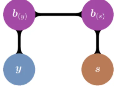
con-nect the longitudinal and the time-to-event processes (Wu and Car-rol, 1988; Wu and Bailey, 1988; Hogan and Laird, 1997a,b, 1998; Vonesh et al., 2006). In this case, both processes are considered as conditionally independent given the random effects b, the parame-ters and hyperparameparame-tersθ, and the covariates x.
f(y,s|b,θ,x) = f(y|b,θ,x)f(s|b,θ,x). (3.4) Figure 3.3 represents this structure of association.
The interpretation for this approach is based on the belief that both processes are governed by a common set of underlying latent indi-vidual characteristics.