DEVELOPMENT OF MICROWAVE DIELECTRIC ALGORITHMS FOR SENSING CORN STALKS
By
GRACE P. OKIROR
Bachelor of Science in Agricultural Engineering Makerere University
Kampala, Uganda 1999
Master of Science in Food Technology Katholieke Universiteit Leuven
Leuven, Belgium 2004
Submitted to the Faculty of the Graduate College of the Oklahoma State University
in partial fulfillment of the requirements for
the Degree of
DOCTOR OF PHILOSOPHY May, 2012
ii
DEVELOPMENT OF MICROWAVE DIELECTRIC ALGORITHMS FOR SENSING CORN STALKS
Dissertation Approved: Dr. Carol L. Jones Dissertation Adviser Dr. Paul R. Weckler Dr. Ning Wang Dr. Marvin Stone Dr. Niels O. Maness Outside Committee Member
Dr. Sheryl A. Tucker Dean of the Graduate College
iii
TABLE OF CONTENTS
Chapter Page
I. INTRODUCTION ... 1
1.1 Background and Motivation ... 1
1.2 Research Goal and Objectives ... 5
II. REVIEW OF LITERATURE... 6
2.1 Overview of microwave dielectric spectroscopy ... 6
2.2 Theory of Dielectric Spectroscopy ... 7
2.3 Practical Microwave Dielectric Algorithms ... 10
2.4 Corn Stalk Characteristics... 12
2.5 Sensing of Corn Stalk Characteristics... 15
2.6 Dielectric Properties of Corn Stalks ... 16
III. METHODOLOGY ... 18
3.1 Simulation of Microwave Scattering Parameters ... 18
3.1.1 Scattering Theory ... 18
3.1.2 Finite Difference Time Domain Method ... 20
3.1.3 Simulation Setup ... 22
3.1.4 Computing Scattering Parameters ... 23
3.2 Experimental Setup ... 24
3.3 Antenna Characteristics ... 26
3.4 Selection of Optimum Antenna Separation ... 26
3.5 Measuring the Effect of Moisture Content ... 28
3.6 Measurement of Corn Stalks ... 28
IV. RESULTS AND DISCUSSION ... 31
4.1 Delrin 500AF Rods S-parameters ... 31
4.1.1 FDTD Simulations ... 31
4.1.2 Comparison with measurements ... 34
4.2 Effect of Moisture Content on S-Parameters ... 39
4.3 Corn Stalk Measurements ... 40
4.3.1 Physical Characteristics... 40
iv
V. CONCLUSIONS AND RECOMMENDATIONS ... 51
REFERENCES ... 53
APPENDICES ... 59
I: Summary of Stalk Physical Properties ... 59
II: Multiple Comparison Tests Using SAS ... 61
v
LIST OF TABLES
Table Page
Table 3.1 Diameters and designations of the Delrin rods ... 18
Table 3.2 Characteristics of the corn sample treatments ... 29
Table 4.1 Water content levels of a soaked foam pad ... 39
Table 4.2 PLS analysis results for average stalk diameter with leaves ... 49
vi
LIST OF FIGURES
Figure Page
Figure 1.1 World corn production data compiled from (FAOSTAT, 2011) ... 2
Figure 2.1 Relationship between corn plant height and grain yield (Yin et al., 2011) ... 14
Figure 2. 2 Relationship between stalk diameter and by-plant corn grain yield at V12 (Kelly, 2011) ... 14
Figure 3.1 Geometrical configuration of scattering from a finite cylinder ... 19
Figure 3.2 Positions of the field components in an FDTD unit cell (Sadiku, 2009) ... 21
Figure 3.3 FDTD Solutions simulation setup ... 22
Figure 3.4 Equipment used and experimental setup ... 25
Figure 3.5 Agilent 85054D Type N calibration kit ... 25
Figure 3.6 Radiation pattern of the waveguide horn antennas used at 2, 9 and 18 GHz from left to right (from the antenna manual) ... 26
Figure 3.7 Effect of separation on attenuation calibration ... 27
Figure 3.8 Effect of tube length on attenuation at 600 mm separation ... 27
Figure 4.1 Typical distribution of the scattering parameters obtained from FDTD simulation. The P’s are obtained from the average power flow values (Equations 3.6 and 3.7) and the S’s are the respective normalized Poynting vectors from equations 3.8. ... 31
Figure 4.2 Variation of attenuation with diameter. D0 was a 'blank' and D1 - D6 were Delrin rods with increasing diameter (table 3.1) ... 32
Figure 4.3 Variation of the return loss with diameter. D0 was a 'blank' and D1 - D6 were Delrin rods as designated in table 3.1. ... 33
vii
Figure 4.4 Source radiation spectrum ... 33 Figure 4.5 Distribution of the coefficients of determination with their respective slopes
slopes (AT – attenuation, RL – Return Loss) of simulated parameters ... 34 Figure 4.6 Variation of relative attenuation with the rod diameters ... 35 Figure 4.7 Variation of the relative return loss with the rod diameters ... 35 Figure 4.8 Distribution of the regression correlation coefficients and slopes (AT –
attenuation, RL – Return Loss) of measured parameters ... 36 Figure 4.9 Variation of the relative return loss with the rod diameters ... 37 Figure 4.10 Distribution of the coefficients of determination with their respective slopes
of the measured phase shift ... 38 Figure 4.11 Variation of attenuation of a water soaked foam pad at different moisture
content values ... 39 Figure 4.12 Variation of the coefficients of determination with their respective slopes for
the water soaked form ... 40 Figure 4.13 The interaction plot for the maximum stalk diameter with date and treatment
plots ... 41 Figure 4.14 The interaction plot for the stalk moisture content with date and treatment
plots ... 42 Figure 4.15 Distribution of phase shift coefficients of determination for whole samples
with time ... 43 Figure 4.16 The distribution of phase shift the coefficients of determination for stripped
samples ... 44 Figure 4.17 The distribution of attenuation coefficients of determination for whole
samples ... 45 Figure 4.18 The distribution of attenuation coefficients of determination for stripped
samples ... 45 Figure 4.19 The distribution of return loss coefficients of determination for whole
samples ... 46 Figure 4.20 The distribution of return loss coefficients of determination for stripped
viii
Figure 4.21 Distribution of the coefficients of determination with their respective slopes of the s-parameters with mean stalk diameter (AT is attenuation, RL is the return loss, E and H are the planes of measurement). ... 47 Figure 4.22 Relationship between coefficients of determination with the probability
values ... 48 Figure 4. 23 Plot of predicted against measured diameter using phase shift of whole
plants ... 50 Figure 4.24 Plot of predicted against measured diameter using attenuation for stripped
1 CHAPTER I
INTRODUCTION
1.1 Background and Motivation
Corn (Zea mays) has had a long history of serving mankind. Originating somewhere in Mexico or Central America thousands of years ago (Buckler IV and Stevens, 2006), it has been under cultivation for more than 4000 years now. It belongs to a grass family Poaceae (Gramineae), along with other agricultural crops like wheat, rice, oats, sorghum, barley and sugar cane. Traditionally, cultivated corn has five main varieties: Z. mays var. Saccharata, otherwise known as sweet corn, Z. mays var. Americana or dent corn which has a soft endosperm, Z. mays var.
Praecox, or flint corn which has a hard endosperm, and Z. mays var. Amylacea or soft corn, predominantly used by American Indians for making flour (Desai et al., 1997). Today, most of the commercially produced corn is a hybrid, specifically selected for different characteristics such as yield (either for grain or forage), drought tolerance, maturation period, pests and pathogens resistance and lodging resistance.
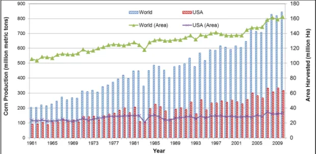
Corn (Zea Mays L.) is the world’s most important grain widely grown in more countries and diverse climates than any other grain or crop (USGC, 2010). In 2010, world production of corn grain exceeded 844 million metric tons (MT), with the leading producers being the United States (316 million MT, 37.4%), China (177 million MT, 21%) and Brazil (56 million MT, 6.6%). Similarly, the total land area cultivated was 161.8 million hectares, with the United States using
2
32.96 million Ha, China 32.52 million Ha and Brazil 12.81 million Ha (FAOSTAT, 2011). Figure 1.1 shows the trends in corn production since 1961.
Figure 1.1 World corn production data compiled from (FAOSTAT, 2011)
Overall, corn production has been steadily increasing throughout the world every year for several decades now. This is attributed to increased acreage, improvements in technology such as seed varieties, fertilizers, pesticides, and machinery, and the adoption of better production practices including reduced tillage, irrigation, crop rotations, and pest management systems (USDA, 2009). Other factors driving up corn production are the seemingly endless list of the crop applications that are constantly being developed.
Corn is utilized as human food, animal feed and in industrial applications. In the developed countries, the largest use of corn and its products is mainly as animal feed. The relative proportions to each end use depend on many factors including geographical location, prevailing agricultural practices and to a lesser extent, the annual crop yield. For example, in Sub-Saharan Africa outside of South Africa, more than 77% of corn is consumed by humans as staple food where it accounts for between 20 and 85% of annual total calorie intake, depending on the country, while only 12% is used as animal feed (Smale et al., 2011). In 2010, the US corn
3
utilization was about 39.4% feed and residual, 34.9% industrial ethanol, 10.5% food, seed and other non-ethanol industrial applications, and 15.4% of the total production was exported (USGC, 2010). The statistics for the rest of the world lie between those of the United States and Sub-Saharan Africa outside South Africa.
Corn is grown over a vast geographical region spanning longitudes 58° North and 40° South on all continents of the world (Runge, 2002) and altitudes ranging from sea level up to 2,200 meters (USDA, 2003); mostly on fertile land with favorable climatic conditions (Desai et al., 1997). For successful cultivation of corn proper tillage, pest and weeds control, availability of moisture and plant nutrients especially nitrogen (N), phosphorus (P) and potassium (K) are paramount (Desai et al., 1997). Other plant nutrients such as zinc, sulfur, iron, boron, copper, manganese and molybdenum in reducing order of significance could be applied to increase grain production based on soil test recommendations (Davis and Westfall, 2009). Availability of these factors in adequate amounts plays a great role in the growth and development of corn and eventually grain yield.
Due to the ever-increasing world demand for corn and its products, scientists and engineers are tasked with ecological intensification (EI) of corn production, the challenge of increasing it to match the current and anticipated demand while reducing its potential negative impacts (Cassman, 1999). Increased production has been achieved by means of several interventions such as development of high yielding and stress-resistant varieties, use of improved cultivation practices, increased acreage, use of fertilizers, herbicides and pesticides, and irrigation. The negative consequences of increased corn production include the health risk to humans and other living organisms by the increased use or exposure to hazardous chemicals; leaching of these chemicals to underground water reservoirs and waterways leading to pollution; reduced quantity and quality of available water due to irrigation; and degradation of habitats and ecosystems due to soil erosion (Runge, 2002).
4
Since the 1950s world food production has increased with the introduction of the use of inorganic fertilizers, especially N (Follett, 2001; Fageria and Baligar, 2003). However, mismanagement of N fertilizers has contributed to excess application especially in developed countries. As a result, the world nitrogen use efficiency in cereals has been reduced to a current of 33% and the unaccounted N (67%) representing annual losses of US$15.9 billion (Raun and Johnson, 1999). In the USA alone, it is estimated that an average of 3500 MT of excess fertilizer nitrate flows into the Mississippi River each day during the spring, amounting to US$391 million per year (Booth, 2006), while Malakoff (1998) estimated an annual loss of US$750 million, with much fo this excess N coming from crop production in the upper Midwest.
Past studies have established a positive relationship between grain yield and Normalized Difference Vegetative Index (NDVI); which is an indirect index for measuring crop biomass and can be used to determine mid-season N fertilizer requirements (Raun et al., 2001; Lukina et al., 2001). Therefore based on this, several studies have indicated that NDVI can be used to predict yield and make precise in-season N recommendations. Research by Raun et al. (2005) showed that an optical sensor based algorithm could be used to calculate in-season potential crop yields in cereals, and to estimate N responsiveness leading to improved N recommendations, thus avoiding losses due to excess N. Teal et al. (2006) demonstrated that a strong relationship existed between corn yield and NDVI at the V8 stage of development and proposed a further normalization using the growing degree days (GDD). Tubaña et al. (2008) established that, using an algorithm to predict mid-season (V8 to V10) N response index (RI) and predicted yield potential (YP0), plus modifying for stand variation using the coefficient of variation (CV) from sensor readings, contributed to an increase in NUE and net return from applied N fertilizer.
Another important corn component that could be used to predict yield and make in-season N recommendation in corn, is stalk diameter. The stalk plays an integral role in the growth and development of a corn plant. It provides support for and the elevation of leaves, flowers and
5
fruits, transport of fluids between the roots and the shoots through xylem and phloem vessels, storage of nutrients and production of new living tissue (Setter and Meller, 1984; Jung and Casler, 2006). Stalk diameter therefore directly correlates with growth and development of corn and grain yield and can be used along with NDVI to predict yield and make N recommendations.
1.2 Research Goal and Objectives
During field production of corn, the number of plants per unit area (plant population density) has been demonstrated to affect the crop yield by several studies (Blumenthal et al., 2003; Overman et al., 2006; Stanger and Lauer, 2006; Singh and Choudhary, 2008). In addition, the stalk size of growing plants provides useful information about the health, vigor and potential yield of the crop. The exact relationship between the population density and yield depends on the crop cultivar, climate, soil type and available nutrients. In order to conduct research on the optimal plant population density, and to ensure that it has been achieved in a planted field, a physical plant count is required. In research studies, manual labor is typically employed. On commercial farms, random sampling and approximation methods are used. An automated, accurate system for on-farm plant measurement is therefore desirable. The overall goal of this research was to investigate the potential of using microwave power scattering in sensing corn stalks in the field. Stalk parameters of interest are diameter, moisture and biomass content. Specifically, the research objectives were:
1. Design and construct an experimental setup for studying corn stalk scattering characteristics
2. Investigate the potential of using microwaves for detecting and counting corn stalks 3. Study the relationship between the microwave scattering parameters of corn stalks and
their diameter, moisture content and biomass content
4. Propose algorithms for sensing corn stalks and estimating their diameter, moisture content and biomass
6 CHAPTER II
REVIEW OF LITERATURE
2.1 Overview of microwave dielectric spectroscopy
Dielectric spectroscopy is one of the non-destructive sensing techniques used for the development of automation systems in rapid quality assessment and large scale material handling and processing. It is based on the investigation of the electromagnetic energy propagating characteristics of a target material. Such characteristics as conductivity, resistivity, capacitance, amplitude, phase and complex permittivity have been studied and found to be related to some characteristics that are fundamental to agricultural and engineering applications (Jha et al., 2011). These dielectric properties are then correlated to the attribute of interest using appropriate mathematical models to derive a reliable algorithm that may be used to develop or compliment the desired technology. Microwaves are a segment of the electromagnetic radiation that travels with frequencies between 300 kHz and 300 GHz, but for practical microwave applications frequencies up to 50 GHz are of interest. Within this frequency range, the electromagnetic waves are non-ionizing, and are therefore safe for industrial applications without altering the constitution of the material under test. Microwave sensors are fast and less susceptible to environmental conditions such as water vapor, dust and high temperatures compared to other sensing technologies (Nyfors and Vainikainen, 1989). In agriculture, dielectric spectroscopy has been used successfully for insect control in wheat, non-destructive sensing of moisture content and other quality attributes, and in microwave heating applications (Nelson, 2006; De los Reyes et al., 2007). This chapter will provide an overview of theoretical and practical aspects of dielectric spectroscopy, with special focus on free-space scattering and application. The second
7
part discusses the practical microwave dielectric algorithms used in agriculture. The last part will discuss the functions of the stalk in corn development, significance of size estimation and previous approaches adopted in automated diameter measurement.
2.2 Theory of Dielectric Spectroscopy
The study of dielectric spectroscopy involves studying the electromagnetic energy propagating characteristics of the material under test and establishing their relationship to the primary attribute of interest. When the material under test is a poor or non-conductor, as is the case with biological materials, it is called a dielectric material (Nyfors and Vainikainen, 1989). When electrical energy propagates in a dielectric, two main phenomena are noted: attenuation due to frictional energy losses in the medium, and phase shift due to a difference in the propagation constant. At the interface of two dielectrics, electrical energy may be reflected or transmitted. All these phenomena which happen to the electrical fields propagating in dielectrics are governed by only two properties: the electrical permittivity and the magnetic permeability of the material. When the material is non-magnetic, as in biological materials, only the permittivity is of primary concern. For practical applications, the dielectric properties of material are expressed in terms of the relative complex permittivity as:
' " | | j
r j e
δ
ε ε
= = −ε
ε
=ε
−(2.1)
Where
ε
ris the permittivity of the material relative to that of free space (ε
0 =8.854x10⁻¹² F/m), often referred to as “permittivity” (ε
);ε
′is the dielectric constant, which represents energy storage in the medium;ε
′′is the dielectric loss factor, which implies energy dissipation in the medium; j= −1 and tanδ ε ε
= ′′/ ′is the loss tangent or dissipation factor (Nelson, 2006). Several factors are known to influence the dielectric properties of biological materials. Foremost is the chemical composition of a given material. The atoms, molecules and ions that may be8
present greatly determine its interaction with an electric field. Although atoms are electrically neutral, they experience electronic polarization in an electric field since the electrons surrounding the nucleus are free to rearrange and redistribute themselves within the confines of the atom in response to the applied electric field. In molecules, this rearrangement in electrons creates an imbalance in charge distribution leading to a presence of a permanent dipole moment. The greater the dipole moment, the more responsive the molecule becomes to electric fields. Ions on the other hand are free to completely migrate within the matrix of the material, leading to ionic conductivity (Nyfors and Vainikainen, 1989). The effect of ionic conductivity in dielectrics can be expressed according to the following equation:
0 " ( )eff " ( )d
σ
ε
ω
ε
ω
ε ω
= + (2.2)Where
ε
eff′′ is the effective dielectric loss factor,ε
d′′
is the loss caused by dipolar interactions of atoms and molecules,σ
is the ionic conductivity (S/m), andω
is the angular frequency of the electric field (Datta et al., 2005). Water, salts and organic solutes are the most prominent chemi-cals determining the dielectric properties of biological materials.The physical state or phase of the material is the second factor influencing its dielectric behavior. Density affects the volume and determines the number of chemical components available to interact with the electric field. Similarly, the dielectric properties of a material in solid or liquid states, granular or powder forms will be different due to changes in bulk density and porosity (De los Reyes et al., 2007). Orientation polarization of polar molecules in more dense material is limited compared to less dense materials due to increased relaxation time (Nyfors and Vainikainen, 1989). The relaxation time (
τ
) is defined as the time taken by polar molecules to be aligned to the applied electric field and its effect on permittivity at a given frequency (ω
) is de-fined by the Debye relation for polar substances:9 ' ' ' 1 rs r r r j
ε
ε
ε
ε
ωτ
∞ ∞ − = + + (2.3)Where:
ε
r′
∞is the permittivity at “infinite” frequency, where orientation polarization cannot take place andε
rs′
is the static permittivity at very low frequencies (or d. c.) (Nyfors and Vainikainen, 1989). In granular or pulverized materials, several models have been proposed to describe their effective dielectric constant in terms of their individual components. The most common mixture equations used in grains are the Complex Refractive Index equation (2.4) and the Landau and Lifshitz, Looyenga equation (2.5):1/ 2 1/ 2 1/ 2 1 1 2 2 ( )
ε
=v( )ε
+v ( )ε
(2.4) 1/3 1/3 1/3 1 1 2 2 ( )ε
=v ( )ε
+v ( )ε
(2.5)Where:
ε
represents the effective complex permittivity of the mixture,ε
1is the permittivity of the medium in which particles of permittivityε
2are dispersed,v
1andv
2are the volume fractions of the respective components, givingv
1+
v
2=
1
(Nelson, 2006). Trabelsi et al. (1998) reported a new density-independent function for predicting moisture content in hard red winter wheat using dielectric properties.The influence of temperature on the dielectric properties of a material directly follows its chemi-cal composition, as temperature thermodynamichemi-cally increases particle mobility and consequently polarization ability. The exact dependence of dielectric properties on temperature is determined by the dielectric relaxation processes prevailing at a given frequency. An increase in temperature reduces the relaxation time leading to an increase in the dielectric constant within the region of dispersion, while the dielectric loss factor will either increase or reduce, depending on whether the operating frequency is higher or lower than the relaxation frequency (Venkatesh and
10
Raghavan, 2004). Similarly, the role of operating frequency on complex permittivity can be dis-cerned from equations (2.2) and (2.3). To that end, the effect of temperature and frequency of the dielectric properties of materials of interest are often studied concurrently (Nelson and Bartley, 2002; Wang et al., 2005).
In view of the foregoing, it is evident that dielectric properties are not unique for a given material. They change with chemical composition, frequency, temperature and the physical phase of the matrix. The data published for standard dielectric properties are limited to pure substances and their mixtures, at prescribed temperatures and frequencies. Attempts to model complex permittivity of food materials with individual chemical components have yielded results of limited practical value (Calay et al., 1995). Ultimately, for practical purposes, an experimental determination of dielectric properties of a target material at prevailing conditions must be carried out.
2.3 Practical Microwave Dielectric Algorithms
Most of the microwave nondestructive evaluation algorithms in the literature are used for internal inspection of physical features of solids or tomography imaging applications. An example of such models is the MUltiple SIgnal Characterization (MUSIC) algorithm which was proposed to estimate and monitor the thickness of a dielectric slab in industrial processes (Abou-Khousa and Zoughi, 2007). This algorithm monitors the complex reflection coefficient and the delay spectrum of a microwave signal using an antenna operating at Ku-band (12.4 – 18 GHz). Laboratory experiments provided an accuracy of at least 95% in measuring Plexiglass and rubber thicknesses of 1.14 and 0.442 cm, respectively. Such an algorithm can serve as a basis for developing a monostatic system for studying corn stalk characteristics in the field.
Eren et al. (1997) developed a microwave testing system consisting of an amplitude stabilized Gunn diode oscillator operating at 10.5 GHz, waveguide horn antennas, a crystal diode detector
11
and attenuators for measuring moisture content in dried fruits. They were able to establish a good relationship between attenuation (dB) and moisture content, with an accuracy of 2 – 3%. It is proposed that this approach can serve as a basis for a bistatic system for measuring corn stalk characteristics in the field.
Trabelsi et al. (2008) proposed three permittivity-based algorithms for determining moisture con-tent and bulk density in granular materials using dielectric properties at 5.8 GHz. Their prototype comprised of a free-space transmission (bistatic) system that measured both phase-shift (
φ
) and attenuation (A). The dielectric constant and loss factor are derived from the following equations for low-loss materials:2
'
1
360
c
d f
φ
ε
= −
(2.6) " ' 8.686 A c d fε
ε
π
− = (2.7)Where
φ ϕ
= −
360
n
,ϕ
is the measured phase angle in degrees, A is attenuation in dB, c is the speed of light in m/s, d is the sample thickness in m and n is an integer selected to eliminate phase ambiguity (Trabelsi et al., 2000). The first algorithm predicted moisture content and bulk density simultaneous as follows: ' " ; and aM b cM dε
ε
ρ
= +ρ
= + (2.8)Where a, b, c and d are linear regression constants determined during calibration and ρ, M are density and moisture content respectively. The prediction equations are as follows:
'
"
'
"
; and
"
'
c
a
d
b
M
bc ad
a
c
ε
ε
ε
ε
ρ
ε
ε
−
−
=
=
−
−
(2.9)12
The second algorithm was designed to predict only bulk density as follows:
"
'
fa
k
ε
ε
ρ
ρ
=
−
(2.10)Where af and kare frequency dependent constants determined during calibration and used for predicting the bulk density in equation (2.11).
' " f f a ka
ε ε
ρ
= − (2.11)The third algorithm was designed to predict moisture content independent of bulk density as follows:
(
")
' af ' "ε
ψ
ε
ε ε
= − (2.12)Where,
ψ
is a density and material independent function related to moisture content as follows:
ψ
=AM +B (2.13)Constants A and B are determined during calibration. All three algorithms were tested and found to predict these quantities with acceptable levels of accuracy (98% for bulk density and 99.5% for moisture content).
2.4 Corn Stalk Characteristics
In order to improve nitrogen use efficiency in agriculture, the normalized difference vegetative index (NDVI) was developed to estimate the mid-season plant N uptake, grain yield potential and thus recommend optimal supplemental N application (Raun et al., 2001; Lukina et al., 2001). Over the years, several modifications have been suggested to improve the accuracy of NDVI in-season grain yield predictions. These modifications include the use of growing degree days
13
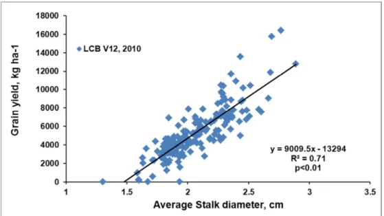
(GDD) (Teal et al., 2006), days from planting (DFP), responsive index (RI), and coefficient of variation (CV) (Tubaña et al., 2008). In addition, other studies have suggested the use of plant characteristics, separately or incorporated into the NDVI algorithm to improve prediction of the potential grain yield in corn. Freeman et al. (2007) obtained good correlations between corn biomass and plant height at V8 – V10 growth stage, while NDVI alone was the best predictor of N uptake. Liu and Wiatrak (2011) obtained statistically significant positive linear correlations between ear height (R2 = 0.58) and plant height (R2 = 0.61) with NDVI; and also showed that grain yield was significantly correlated with ear height. Yin et al. (2011) investigated the potential of using plant height at different stages of development to directly predict corn yield. Figure 2.1 shows typical results they obtained over a period of three years. Overall, better predictions were obtained at V10 and V12 growth stages. Kelly (2011) also studied the effect of both plant height and diameter on corn yield. Figure 2.2 shows the relationship between by-plant grain yield and stalk diameter at V12 stage of development. These findings underscore the need to include plant growth characteristics in the NDVI algorithms in order improve to NUE.
14
Figure 2.1 Relationship between corn plant height and grain yield (Yin et al., 2011)
Figure 2. 2 Relationship between stalk diameter and by-plant corn grain yield at V12 (Kelly, 2011)
15
The second aspect of corn stalk properties related to production is the need to establish plant population density. The plant population density affects lodging resistance, pest infestation and grain yield of corn and it is affected by several factors including variety, seed quality, soil fertility and climate (Lauer and Stanger, 2007; Echezona, 2007). Nafziger (1996) demonstrated that a missing plant in a row would lead to a reduction of at least 53% in by-plant corn yield. In order to optimize the yield, an accurate method for determining the plant population in the field is desirable. Even when the population density is fixed, the row spacing and interplant distances within the row can affect the final yield (Barbieri et al., 2000). Easton and Easton (1996) patented a mechanically actuated, human-powered system that counts and measures the spacing of young row crops with the help of a microprocessor. Nichols (2000) also patented a device which uses a moisture sensor for the detection and counting of row crops during harvest. These systems have practical limitations in use and have not been widely adopted.
2.5 Sensing of Corn Stalk Characteristics
Several studies on non-destructive sensing of agricultural crops and corn in particular, have been reported. Guyer et al. (1986) provided a general overview of the main principles of machine vision and image processing, and developed a system of using digital images for identification of corn, soybeans, tomatoes and various grasses at very early stages of development. Jia et al. (1990) investigated the potential of using machine vision for identifying the leaves and locating the center of corn plants. They used a CCD camera with separate color and composite outputs (red, green, blue) along with a computer and appropriate hardware for image processing. Success in locating individual corn plants was achieved, but challenges were faced with fixing the centers due to overlapping or partial leaf images. This system would be practical for target sprays for weed control.
Shrestha and Steward (2003) developed an image processing algorithm for counting corn plants using a digital video camera with an accuracy of about 90%. Later, they investigated the
16
possibility of improving the accuracy of this system by including the shape and size of the plant canopy (Shrestha and Steward, 2005). The accuracy increased to 92% and they noted that the younger the plants, the better the results. Luck et al. (2008) investigated the use of low cost infrared ranging sensors for counting corn stalks. They calibrated the sensors at distances between 5 and 112.5 cm from the target in the laboratory and tested them in a 30-m corn row with 136 plants approximately 1 m high (V7 –V9 growth stage) and average stem diameter of 2.85 cm. They concluded that the setup was able to count the stalks between 20 and 60 cm from the sensors with an accuracy of 95%. These machine vision attempts have faced serious challenges such as varying outdoor lighting, overlapping canopies and weed interference, which are difficult to overcome. Jin and Tang (2009) proposed an algorithm that employed real-time stereo (3D) vision to map plant skeleton structures. They used an active stereo vision system comprising a two lens monochrome camera with a speed of 30 frames per second. They reported a corn plant detection accuracy of 96.7% at a V2 – V3 growth stage. A prototype corn stalk counter utilizing laser sensors has recently been developed in an attempt to overcome the drawbacks of machine vision based technologies (Grift, 2010).
2.6 Dielectric Properties of Corn Stalks
Although numerous dielectric studies have been done on corn, most of them focused on grain with a view of determining moisture content and other internal quality attributes (Nelson, 1978; Nelson and You, 1989; Trabelsi et al., 1997; Sacilik and Colak, 2010). El-Rayes and Ulaby (1987) conducted the dielectric measurements of corn stalks and leaves with the moisture content range of 8 – 83%, along with other plants using an open-ended coaxial probe in the range 0.2 – 20 GHz. They developed some models to describe the dielectric behavior of corn leaves at different moisture content values, but no models for corn stalks were described (Ulaby and El-Rayes, 1987). There have not been any further studies in dielectric properties of corn stalks reported in literature.
17
The scope of this work involved a feasibility investigation of the potential of using free-space microwave scattering parameters for sensing corn stalks in the field. Testing began with theoretical simulations of scattering using dielectric rods as a first order model, followed by actual measurements of these rods. During the second phase, the microwave power attenuation, phase shift, and return loss of actual corn stalks during growth and development were measured at the laboratory scale, along with the diameters and moisture content. Finally, statistical analysis of all the data obtained was conducted to derive useful patterns and recommendations for subsequent research.
18 CHAPTER III
METHODOLOGY
3.1 Simulation of Microwave Scattering Parameters
In order to simulate the free-space scattering parameters of corn stalks, Delrin rods were used as a first order model. Delrin 500AF is a cylindrical non-dispersive plastic dielectric with a dielectric constant of 3.1 and dissipation factor of 0.009. Six rods of different diameters within the order of typical corn stalks and constant lengths of 410 mm were chosen as shown in table 3.1. The length was chosen to represent the practical minimum for simulations using the available setup.
Table 3.1 Diameters and designations of the Delrin rods
Designation D1 D2 D3 D4 D5 D6
Diameter (mm) 12.72 15.88 19.12 22.24 25.41 31.88
A model was developed that describes free-space scattering of finite cylindrical structures with varying diameters in the frequency range of 1 – 18 GHz (wavelengths of 17 – 300 mm). This approach has been used before in modeling the scattering characteristics of tree branches (Seker and Schneider, 1988).
3.1.1 Scattering Theory
Several approaches have been used to model free-space scattering of electromagnetic waves. Kahnert (2003) provided a comprehensive review of the application of the various numerical methods to electromagnetic (EM) scattering. There are two main approaches that have been pursued in the past to model EM scattering from a finite cylindrical dielectric object, the use of
19
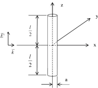
the method of moments (MoM) and the use of the FDTD method. Nevertheless, each of these methods is founded on the same basic principles. Figure 1 below illustrates the geometrical set up.
Figure 3.1 Geometrical configuration of scattering from a finite cylinder
Consider a transverse magnetic (TM) polarized incident time harmonic plane wave ( Ei ) approaching the cylinder in the
k
direction (x, in this case). The rod diameter and length are aand lrespectively. The total field at any point (r ) in space is given by:
( )
i( )
s( )
E r =E r +E r (3.1)
Where Es
( )
r is the scattered field. Equation (3.1) is a summary of the principle of superposition. However, in the case of bistatic scattering, it is also required to apply the same equation inside the cylinder. The scattered field can be generated from an equivalent electric current radiating in an unbounded free space with the following current density (Richmond, 1966):( )
0( 1)
s r
20
Where,
ε
ris the relative permittivity of the scatterer andε
0 is the absolute permittivity of free space. Equations (3.1) and (3.2) when applied to the geometry of figure 1 can be combined and expressed as follows (Uzunoglu et al., 1978; Papayiannakis and Kriezis, 1983):( )
2(
1)
(
1 2)
(
,) ( )
.( )
r i
V
E r −k
ε
−∫
+k−∇∇ G r r′ E r dv′ ′=E r (3.3)Where, kis the wave number,
r
′
is the position vector of the source point,1
is the unit dyadic andG r r
( , )
′
is the free space Green’s function. Before proceeding with solving equation (3.3), an assumption regarding the scatterer’s dimensions has to be made, whether it is smaller or larger in relation to the wavelength of the incident fields. Taking the ratio 2π
a/λ
as a guide and assuming the worst case scenario, the value of 0.266 obtained from the smallest Delrin rod is not very much smaller than unity and so the model of large dimensions is taken for the current research (Uzunoglu et al., 1978). Appropriate numerical techniques are then employed to simplify Equation (3.3), which is solved twice, first to determine the fields inside the cylinder, and then for the scattered fields.3.1.2 Finite Difference Time Domain Method
The Finite Difference Time Domain method (FDTD) was original developed for EM computations and employs center-difference representations of the continuous partial differential equations to create iterative numerical models of wave propagation. The fundamental idea is to solve Maxwell’s equations in time and space (Sadiku, 2009). In an isotropic medium, Maxwell’s equations can be simplified to two interdependent expressions as in equations (3.4).
H E t E H E t
µ
σ
ε
∂ ∇ × = − ∂ ∂ ∇ × = + ∂ (3.4)21
Where
E
andH
are the time dependent electric and magnetic fields respectively,µ
is the magnetic permeability,ε
is electrical permittivity,σ
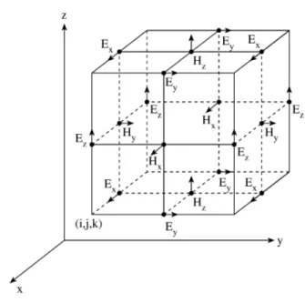
is the electric conductivity, t is time and ∇ is vector differential operator. In Cartesian coordinates, each curl operator results into three scalar equations, which are solved using the second order center-difference approximation to determine the fields. In FDTD, these equations are solved in a unit three dimensional lattice cell in which all the fields must be computed sequentially in alternate time steps as shown in figure 3.2, where,
i jand kare integers. Key steps in FDTD implementation is selecting the correct time and space steps to ensure computational accuracy and stability, and specifying appropriate lattice truncation conditions.
Figure 3.2 Positions of the field components in an FDTD unit cell (Sadiku, 2009)
The FDTD method was chosen due to its relative conceptual simplicity and ease of implementation, especially in inhomogeneous media and arbitrary geometries, so that no separate computational relations are required to compute the fields inside and outside the dielectric rods. The problem usually encountered in the application of FDTD to cylindrical objects is the programming of the curved edges, which has traditionally been done by staircasing. This has been
22
noted to introduce some errors and discouraged its application to rough or jagged surfaces (Jurgens et al., 1992). For the purpose of dielectric rods, the staircase approach does not introduce significant errors. In addition, a contour path algorithm suggested by Jurgens et al. (1992) can be used to completely eliminate these errors.
The FDTD method generates electric and magnetic fields distributed in space and time over the defined simulation region. These values can then be used to compute power flow by integration of Poynting vectors over the monitor cross-section and frequency distributions using Discrete Fourier Transforms. Finally, scattering parameters can be deduced using relevant theoretical relationships. Therefore, the FDTD method was used to simulate Delrin rods.
3.1.3 Simulation Setup
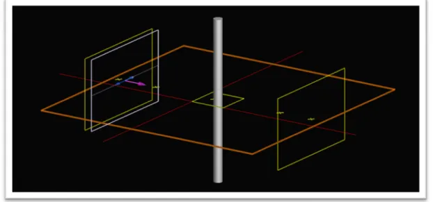
Special software for FDTD simulations (FDTD Solutions, Lumerical Solutions, Inc., Vancouver, Canada) was used to complete this task. Figure 3.3 shows the basic simulation setup.
Figure 3.3 FDTD Solutions simulation setup
The grey cylinder represents the Delrin rod whose electrical properties were specified in the materials database and the radius was varied with each simulation. The blue and purple lines represent the span and direction of the electromagnetic field source (positive x in this case),
23
which was specified here as a plane wave source with dimensions of the waveguide horn antennas indicated by the white box over the 1 – 18 GHz frequency range. The green crosses and boxes are field monitors used to store the desired variables. The crosses are point monitors which store only vector quantities while the boxes are spatial monitors that can also store scalar integral quantities such as output power. The reflection monitors were placed 1 cm behind the source point while transmission monitors were placed 5 cm in front of the dielectric rod. In addition, a field distribution monitor was placed to capture the patterns around the rod. The red lines are the x and y axes cursor positions while the orange ring represents the FDTD simulation region. Due to memory limitations of the trial license used, it was not possible to simulate the full length of the rod, so an infinite length of the dielectric rod was assumed which was specified as periodic in the simulation region for the + and - z directions.
3.1.4 Computing Scattering Parameters
Two sets of s-parameters were monitored: S11 for reflection (return loss) and S21 (attenuation) for transmission. These parameters are usually computed using the following equations:
11( ) 20 log10 S dB = Γ (3.5) 21( ) 20 log10 S dB = Τ (3.6)
Where, Γand Τare the reflection and transmission coefficients, respectively (Pozar, 2005; Nyfors and Vainikainen, 1989). Since these parameters were collected over free-space, they could be estimated using average power densities at the observation regions, using the following expressions (Nyfors and Vainikainen, 1989):
11
10 log
10Return Loss
R S
P
S
dB
P
=
= −
(3.7)24 21
10 log
10Attenuation
T SP
S
dB
P
=
=
(3.8)Where,
P
R,P
S andP
T are average power densities at the reflected, source and transmitted regions respectively. The return loss is expressed as a positive number for consistency and takes on values from 0 for total power reflection to infinity for a matched load. Equations (3.7) and (3.8) were used to compute the scattering parameters from simulation results. Additionally, the Poynting vectors which represent directional complex power density at the observation point were computed according to the following equations (Balanis, 1989):* * * x y z y z x z x y S E H S E H S E H = × = × = × (3.9)
Where, E and Hare the electric and magnetic field intensities respectively and the asterisk (*) denotes complex conjugation.
3.2 Experimental Setup
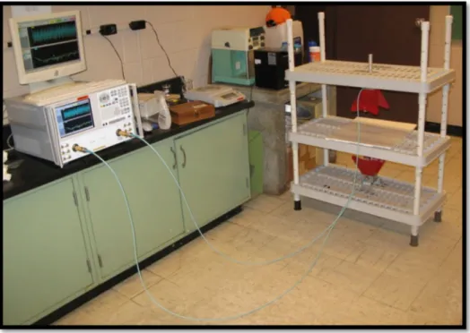
Figure 3.4 shows the equipment and setup used for all the practical measurements conducted in this study. Measurements were carried out using double-ridged waveguide horn antennas (Model 3117, ETS-Lindgren, Cedar Park, TX) connected to a vector network analyzer (Agilent N5230A PNA-L) using two low loss coaxial cables 2.5 m long (UTiFLEX®, Micro-Coax, PA). The antennas were mounted vertically on a specially designed PVC frame and held at 600 mm apart with the samples suspended midway. The measurement system was set to take measurements of S21 parameters attenuation (dB), phase shift (degrees), forward return loss (S11) in dB and reverse return loss (S22) in dB at 401 linearly spaced points between 1 and 18 GHz. Each sample was measured twice, on the E and H plane, and three readings were taken and their mean was
25
reported. The setup was calibrated following the SOLT (Short-Open-Load-Through) approach using the Agilent 85054D mechanical standards at the measurement plane (Figure 3.5).
Figure 3.4 Equipment used and experimental setup
26
3.3 Antenna Characteristics
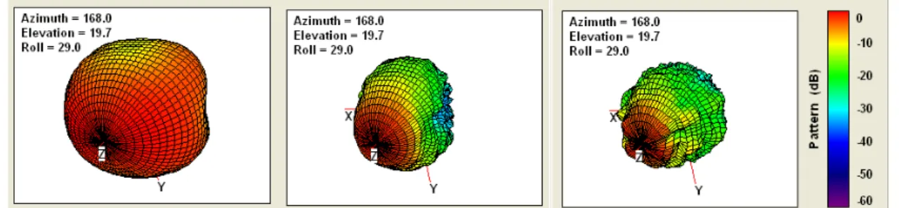
The Model 3117 Double Ridged waveguide antennas used in this study are designed to operate at 1 – 18 GHz with a maximum power rating of 400 Watts, 50 ohm impedance, and a single lobe radiation pattern for the full spectrum. They are linearly polarized with a transverse electromagnetic field (TEM) fed by Type-N coaxial connection. The voltage standing wave ration (VSWR) and Gain reported in the user guide show slightly reduced performance below 1.5 GHz, but these are compensated by the very high half power beam widths at lower frequencies. Figure 3.6 shows the reported radiation patterns.
Figure 3.6 Radiation pattern of the waveguide horn antennas used at 2, 9 and 18 GHz from left to right (from the antenna manual)
3.4 Selection of optimum antenna separation
A preliminary experiment was designed to minimize direct antenna coupling and reduce the effect of variable lengths of the objects in the antenna field of view. Direct coupling is known to cause measurement errors when the transmitting and receiving antennas are very close to each other (McEwan, 2000). Seven clear plastic tubes of 25.4 mm external diameter and variable lengths (320, 400, 500, 600, 700, 800 and 900 mm) were filled with water to increase their permittivity and placed at the center of the antennas and the scattering parameters monitored with varying antenna separations (200, 300, 400, 500 and 600 mm). The purpose was to determine the separation at which the length of the tubes does not significantly affect the scattering parameters and the echo signal due to direct coupling does not significantly affect the calibrations. Figure 3.7
27
shows the effect of separation on calibration while figure 3.8 shows the effect of tube length on attenuation at 600 mm separation.
Figure 3.7 Effect of separation on attenuation calibration
Figure 3.8 Effect of tube length on attenuation at 600 mm separation
0 2 4 6 8 10 12 14 16 18 20 -7 -6 -5 -4 -3 -2 -1 0 1 2 Frequency (GHz) A tt e n u a ti o n ( d B ) 20 cm 30 cm 40 cm 50 cm 60 cm 0 2 4 6 8 10 12 14 16 18 20 -6 -5 -4 -3 -2 -1 0 1 2 3 Frequency (GHz) A tt e n u a ti o n ( d B ) 32 cm 40 cm 50 cm 60 cm 70 cm 80 cm 90 cm
28
It can be seen from figure 3.5 that at separations higher than 300 mm, the calibration is steady near zero attenuation as theoretically expected. However, the calibration at 200 mm is quite noisy, especially at very low frequencies. This indicates the high echo signal at this separation. For the tube lengths, it was observed that at lower separations, the tube lengths did not produce visually significant differences in attenuation at lower frequencies (below 10 GHz), but became unsteady as the frequency increased. This pattern tended to reverse as the separation increased. Between 400 and 600 mm separations, very short (320 mm) and very long (900 mm) tubes deviated. Within these two extremes, the tube length did not matter. These patterns were consistent for all the four scattering parameters measured. A separation of 600 mm and sample length of 410 mm were then selected to reflect possible field applications in the future.
3.5 Measuring the Effect of Moisture Content
Since water is the main component in biological materials, it was vital to investigate its effect on s-parameters independent of the biochemical interactions that are present in corn stalks. This was done by using a 30 mm x 40 mm x 430 mm strip of a bio-based foam pad. The dry strip was weight and the s-parameters measured. Following this, water was soaked into the strip at 5 gram interval until complete saturation at around 77% moisture content on a wet basis. Both absolute moisture (moisture mass, grams) and the wet-basis moisture content were used in analysis.
3.6 Measurement of Corn Stalks
The corn plants used in this study were cultivated at the Efaw agronomy research station in Stillwater, Oklahoma. The corn was hybrid number Dekalb DKC 52-59, planted on May 26, 2011, divided into four plots with treatments of population density and nitrogen application rate in combination. Each plot was four rows wide and 21 m long. Table 3.2 shows the different plot treatments. The crop was uniformly irrigated as needed due to drought severity during the growing season.
29
Table 3.2 Characteristics of the corn sample treatments
Plot Number Population Density (plants/ha) Nitrogen rate (kg/ha)
I 69,188 89.6
II 49,420 179.2
III 49,420 89.6
IV 49,420 0
Data collection started at around the V8 stage of development on June 22, 2011 and continued every 2 to 4 days for ten times till VT, after the plants tasseled and stopped increasing in diameter, on July 19, 2011. On each sampling date, 5 plants from each treatment were dug out using a shovel and transferred to a labeled plastic bucket where they were moderately watered, transported to the laboratory and stored till dielectric measurement. Prior to use, the VNA was powered up and left to warm up for at least 30 minutes before it was calibrated and used. The calibration data (blanks) were stored and another blank reading was taken after the measurement session. The initial and final calibration readings were compared to ascertain the stability of the measurement system.
To measure each sample, it was removed from the bucket, cut at ground level, wiped dry and clean, and then trimmed down approximately 420 mm for longer plants. Thereafter, the plant was placed on the measuring platform midway between the antennas. The four scattering parameters were measured in triplicate and two perpendicular orientations (E and H planes of the antennas). This step was repeated with the same sample stripped off leaves, to determine the effect of leaves on the measured parameters. Following this, a length of about 250 mm was cut off from the bottom end of the stalk and the major and minor diameters were measured using a pair of digital calipers between 50 and 100 mm from the ground level, avoiding the nodes. The average diameter was computed from these readings and recorded. Subsequently, a sample was weighed and oven-dried at 103°C for 24 hours, then weighed again. The wet-basis moisture content was
30
computed using equation (3.10) and the biomass content obtained as the remaining fraction after subtracting the moisture content. Data analysis for determining the relationships between the different diameters and scattering parameters was done using simple linear regression at 401 individual frequency points with MATLAB® R2010b (The MathWorks, Inc., Natick, MA) and comparative analyses were done using SAS 9.2 (SAS Institute Inc., Cary, NC).
(%)
i f100
iM
M
MC
M
−
=
×
(3.10)Where, MCis the wet-basis moisture content,
M
iis the initial mass (g) and Mfis the final mass (g) of the sample.31 CHAPTER IV
RESULTS AND DISCUSSION
4.1 Delrin 500AF Rods S-parameters
4.1.1 FDTD Simulations
This section presents the results from the FDTD simulations and their comparison with the data obtained by physically measuring the Delrin rods. Figure 4.1 shows the typical patterns of the parameters obtained from the simulation. In addition, the Poynting vectors were used to compute the directional power density distributions.
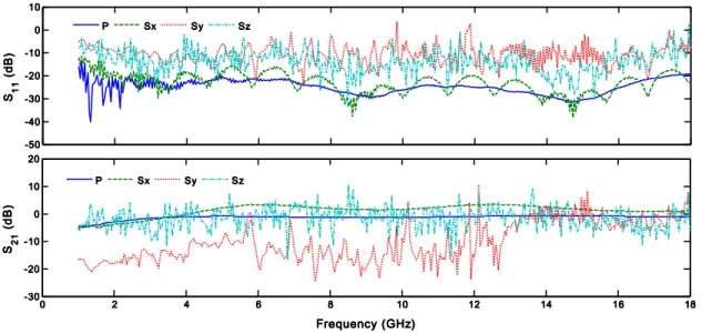
Figure 4.1 Typical distribution of the scattering parameters obtained from FDTD simulation. The P’s are obtained from the average power flow values (Equations 3.6 and 3.7) and the S’s are the respective normalized Poynting vectors from equations 3.8.
It is observed from figure 4.1 that for each s-parameter, there is an approximate representative Poynting vector. This indicates that most of the power travels in a specific direction (x-direction
-50 -50 -50 -50 -40 -40 -40 -40 -30 -30 -30 -30 -20 -20 -20 -20 -10 -10 -10 -10 0 0 0 0 10 1010 10 SSSS1 1 1 1 1 1 1 1 ( d B ) ( d B ) ( d B ) ( d B ) P PP P SxSxSxSx SySySySy SzSzSzSz 0 00 0 2222 4444 6666 8888 10101010 12121212 14141414 16161616 18181818 -30 -30 -30 -30 -20 -20 -20 -20 -10 -10 -10 -10 0 0 0 0 10 10 10 10 20 20 20 20 Frequency (GHz) Frequency (GHz)Frequency (GHz) Frequency (GHz) SSSS 2 1 2 1 2 1 2 1 ( d B ) ( d B ) ( d B ) ( d B ) P PP P SxSxSxSx SySySySy SzSzSzSz
32
for reflected power and x, z for transmitted power). Furthermore, there is more transmitted power (around -5 dB, depending on the frequency) than reflected power (about -25 dB). However, these values do not account for the total power flow in the region. This is due to the fact that the scatterer (Delrin rod) is finite and small, and so the amount of power flow depends on the location, orientation and size of the monitors. The monitors used in the simulation were 5 x 5 cm squares centered on the x axis in the y-z direction. Therefore, it was not possible to capture all the power flow in a given direction. Nevertheless, the setup provided a reasonable simulation of the physical measurement setup, and since the monitor points and regions were fixed during the simulation of the different rod diameters, the values obtained could be reliably used for estimating diameters. The variations of the respective s-parameters with diameter for the different rods are shown in figures 4.2 and 4.3.
Figure 4.2 Variation of attenuation with diameter. D0 was a 'blank' and D1 - D6 were Delrin rods with increasing diameter (table 3.1)
0 00 0 2222 4444 6666 8888 10101010 12121212 14141414 16161616 18181818 -10 -10-10 -10 -9 -9 -9 -9 -8 -8 -8 -8 -7 -7 -7 -7 -6 -6 -6 -6 -5 -5 -5 -5 -4 -4 -4 -4 -3 -3 -3 -3 -2 -2 -2 -2 -1 -1 -1 -1 0 0 0 0 Frequency (GHz) Frequency (GHz) Frequency (GHz) Frequency (GHz) A tt e n u a ti o n ( d B ) A tt e n u a ti o n ( d B ) A tt e n u a ti o n ( d B ) A tt e n u a ti o n ( d B ) D0 D0 D0 D0 D1D1D1D1 D 2D 2D 2D 2 D3D3D3D3 D 4D 4D 4D 4 D5D5D5D5 D6D6D6D6
33
Figure 4.3 Variation of the return loss with diameter. D0 was a 'blank' and D1 - D6 was Delrin rods as designated in table 3.1.
The attenuation was observed to increase with diameter while the return loss decreased with diameter, which is expected according to theory. However, the peak attenuation occurs at progressively reducing frequency. Also, for both parameters there was no discernible distinction between the blank and samples at frequencies below 3 GHz. This may be attributed to the rather small field intensities at these frequencies as indicated by the Gaussian source radiation spectrum (figure 4.4).
Figure 4.4 Source radiation spectrum 0 0 0 0 2222 4444 6666 8888 10101010 12121212 14141414 16161616 18181818 0 00 0 5 55 5 10 10 10 10 15 15 15 15 20 20 20 20 25 25 25 25 30 30 30 30 35 35 35 35 40 40 40 40 45 45 45 45 50 50 50 50 Frequency (GHz) Frequency (GHz) Frequency (GHz) Frequency (GHz) R e tu rn L o s s ( d B ) R e tu rn L o s s ( d B ) R e tu rn L o s s ( d B ) R e tu rn L o s s ( d B ) D0 D0 D0 D0 D 1D 1D 1D 1 D 2D 2D 2D 2 D3D3D3D3 D4D4D4D4 D5D5D5D5 D 6D 6D 6D 6
34
In order to determine the diameter predictive power of the S-parameters, a simple linear regression was carried out at the individual frequencies of the parameters versus rod diameters. Figure 4.5 shows the frequency distribution of the regression coefficients of determination and slopes.
Figure 4.5 Distribution of the regression coefficients of determination with respective slopes slopes (AT – attenuation, RL – Return Loss) of simulated parameters
The attenuation coefficients of determination and slopes both have peaks around 6 GHz, indicating that to be a good region for attenuation measurements. The return loss shows random correlation peaks between 1 and 3 GHz, with corresponding slope peaks at the same neighborhood. These findings were confirmed by repeating the simulation over 1 – 10 GHz frequency, where the pattern obtained was unchanged. It is noteworthy that the nonzero slopes are negative for attenuation, indicating increase with diameter while those of the return loss are positive, indicating that larger diameter rods have a smaller return loss, since more power is reflected back to the transmitting antenna.
4.1.2 Comparison with Measurements
The variations of the measured S-parameters with Delrin rod diameters are shown in figures 4.6 and 4.7 respectively. The measurements for the H and E plane were not remarkably different.
0 0 0 0 2222 4444 6666 8888 10101010 12121212 14141414 16161616 18181818 0 00 0 0.25 0.250.25 0.25 0.5 0.50.5 0.5 0.75 0.750.75 0.75 1 11 1 RRRR 2222 0 0 0 0 2222 4444 6666 8888 10101010 12121212 14141414 16161616 18181818-1-1-1-1 0 0 0 0 1 1 1 1 S lo p e S lo p e S lo p e S lo p e Frequency (GHz) Frequency (GHz) Frequency (GHz) Frequency (GHz) AT R2 RL R2 AT Slope RL Slope
35
Figure 4.6 Variation of relative attenuation with the rod diameters
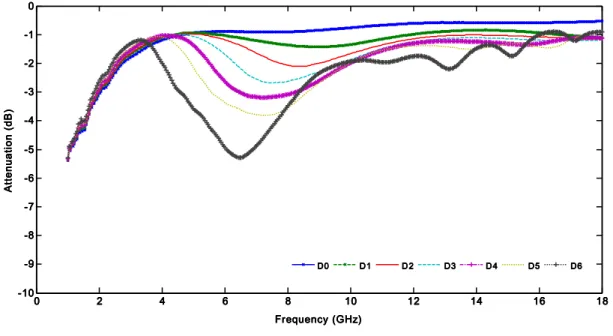
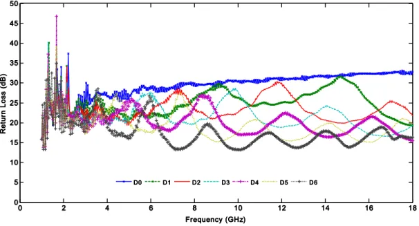
Figure 4.7 Variation of the relative return loss with the rod diameters
A comparison of figures 4.2 and 4.3 with their respective measured values in figures 4.6 and 4.7 reveals that the magnitudes of the measured values are larger than the simulated values. This is due to the fact that the simulation assumed a lossless dielectric rod of infinite length, which is not true in the actual measurement. The relative attenuation follows the same pattern as the simulated
0 00 0 2222 4444 6666 8888 10101010 12121212 14141414 16161616 18181818 -10 -10-10 -10 -8 -8 -8 -8 -6 -6 -6 -6 -4 -4 -4 -4 -2 -2 -2 -2 0 00 0 2 22 2 Frequency (GHz) Frequency (GHz) Frequency (GHz) Frequency (GHz) R e la ti v e A tt e n u a ti o n ( d B ) R e la ti v e A tt e n u a ti o n ( d B ) R e la ti v e A tt e n u a ti o n ( d B ) R e la ti v e A tt e n u a ti o n ( d B ) D1 D1 D1 D1 D2D2D2D2 D 3D 3D 3D 3 D4D4D4D4 D 5D 5D 5D 5 D 6D 6D 6D 6 0 00 0 2222 4444 6666 8888 10101010 12121212 14141414 16161616 18181818 -20 -20 -20 -20 -10 -10 -10 -10 0 00 0 10 10 10 10 20 20 20 20 30 30 30 30 40 40 40 40 50 50 50 50 60 60 60 60 70 70 70 70 Frequency (GHz) Frequency (GHz)Frequency (GHz) Frequency (GHz) R e la ti v e R e tu rn L o s s ( d B ) R e la ti v e R e tu rn L o s s ( d B ) R e la ti v e R e tu rn L o s s ( d B ) R e la ti v e R e tu rn L o s s ( d B ) D1 D1D1 D1 D2D2D2D2 D3D3D3D3 D4D4D4D4 D5D5D5D5 D6D6D6D6
36
values, but the frequency region is shifted farther to the right. This may be attributed to the difference between the theoretical and the actual signal sources used. Unlike the uniform plane wave source used in the simulation, the radiation pattern of double –ridged waveguide horns is not uniform throughout the 1 – 18 GHz bandwidth. The radiation pattern of the antennas tends to deteriorate at higher frequencies (typically above 12 GHz) due to random minute gaps and geometric imperfections that may occur during construction and the possible existence of higher order modes (Bruns et al., 2003). Furthermore, the physical measurements were not carried out in an anechoic chamber, though any environmental reflections were normalized during system calibration. The relative return loss similarly displays the simulated pattern, but the measured values have more rapidly decaying amplitudes with increasing frequency. The corresponding regression correlation coefficients and slopes at the respective frequencies for the measured values are shown in figure 4.8.
Figure 4.8 Distribution of the regression correlation coefficients and slopes (AT – attenuation, RL – Return Loss) of measured parameters
0 00 0 2222 4444 6666 8888 10101010 12121212 14141414 16161616 18181818 0 00 0 0.2 0.2 0.2 0.2 0.4 0.4 0.4 0.4 0.6 0.6 0.6 0.6 0.8 0.8 0.8 0.8 1 11 1 RRRR 2222 0 00 0 2222 4444 6666 8888 10101010 12121212 14141414 16161616 18181818-1-1-1-1 -0.5 -0.5-0.5 -0.5 0 00 0 0.5 0.50.5 0.5 1 11 1 1.5 1.51.5 1.5 S lo p e S lo p e S lo p e S lo p e Frequency (GHz) Frequency (GHz) Frequency (GHz) Frequency (GHz) AT R2 RL R2 AT Slope RL Slope
37
The regression correlation coefficients and slopes of the relative attenuation are found to follow the pattern of the simulated values, both peaking occurring at the same frequency range with an offset at 12 GHz already noted. The return loss values are also found to be consistent with the simulations, peaks of both coefficients and slopes occurring together between 2 and 4 GHz.
Additionally, phase-shift in transmission (S21) measurements for the different rod diameters were made for both E and H plane orientation of the rods. Figure 4.9 shows the variation of phase shift with rod diameter.
Figure 4.9 Variation of the relative return loss with the rod diameters
It is observed that absolute value of the phase shift increases with diameter and also provides a higher diameter resolution between 2 and 12 GHz compared to both attenuation and return loss measurements. Figure 4.10 shows the distribution of the linear regression statistics.
0 00 0 2222 4444 6666 8888 10101010 12121212 14141414 16161616 18181818 -60 -60 -60 -60 -50 -50 -50 -50 -40 -40 -40 -40 -30 -30 -30 -30 -20 -20 -20 -20 -10 -10 -10 -10 0 0 0 0 10 1010 10 Frequency (GHz) Frequency (GHz) Frequency (GHz) Frequency (GHz) R e la ti v e P h a s e S h if t ( R e la ti v e P h a s e S h if t ( R e la ti v e P h a s e S h if t ( R e la ti v e P h a s e S h if t (°°°° )))) D1 D1 D1 D1 D2D2D2D2 D 3D 3D 3D 3 D4D4D4D4 D5D5D5D5 D 6D 6D 6D 6
38
Figure 4.10 Distribution of the coefficients of determination with their respective slopes of the measured phase shift
The coefficients of determination are consistently high (greater than 0.95) for frequencies between 2 and 10 GHz for both orientations, but rapidly deteriorate at higher frequencies. This is due to the fact that above 10 GHz (wavelength = 30 mm), the wavelengths of the incident fields are within the magnitude of the dielectric rods and therefore phase shift ambiguity occurs. The regression slopes have peaks at frequencies 6 and 8 GHz, which incidentally coincide with the peaks of the simulated attenuation. It is therefore concluded that all three of the s-parameters are viable for measuring diameters. However, comparing the maximum absolute values of the slopes of the measured s-parameters, the attenuation has 0.5, return loss has 1.2 and the phase shift has 2.1, shows that phase shift is the best parameter for estimating diameter, since the slope is directly related to the measurement resolution.
0 0 0 0 2222 4444 6666 8888 10101010 12121212 14141414 16161616 18181818 0 00 0 0.2 0.2 0.2 0.2 0.4 0.4 0.4 0.4 0.6 0.6 0.6 0.6 0.8 0.8 0.8 0.8 1 11 1 RRRR 2222 0 0 0 0 2222 4444 6666 8888 10101010 12121212 14141414 16161616 18181818-3-3-3-3 -2 -2 -2 -2 -1 -1 -1 -1 0 0 0 0 1 1 1 1 2 2 2 2 S lo p e S lo p e S lo p e S lo p e Frequency (GHz) Frequency (GHz)Frequency (GHz) Frequency (GHz) Phase E R2 Phase H R2 Phase E Slope Phase H Slope