Density Functional Theory (LEDO-DFT):
Development and Implementation of Algorithms,
Optimization of Auxiliary Orbitals and
Benchmark Calculations
Den Naturwissenschaftlichen Fakult¨
aten
der Friedrich–Alexander-Universit¨
at Erlangen–N¨
urnberg
zur
Erlangung des Doktorgrades
vorgelegt von
Andreas Walter G¨
otz
von den Naturwissenschaftlichen Fakult¨
aten
der Universit¨
at Erlangen–N¨
urnberg
Tag der m¨undlichen Pr¨ufung: 09. August 2005 Vorsitzender der
Promotionskommission: Prof. Dr. D.-P. H¨ader Erstberichterstatter: Prof. Dr. A. G¨orling Zweitberichterstatter: Prof. Dr. P. Otto
mondo `e de’ maggiori e de’ pi´u nobil problemi che sieno in natura . . .
(Let us remember, please, that the search for the con-stitution of the world is one of the greatest and noblest problems presented by nature . . . )
Galileo Galilei,
Dialogo sopra i due massimi sistemi del mondo
It is a great pleasure to be able to thank all the people who have helped me in various ways with this dissertation, and whose support has been invaluable over the past three and a half years.
In the first place I would like to thank my supervisor and academic teacher Prof. Dr. Bernd A. Heß (†) who offered me the opportunity to work in the interesting field of density fitting methods in density functional theory. He has always been a faithful source of knowledge and inspiration. I deeply appreciate his diverse and generous support and the excellent working conditions he provided at the Chair of Theoretical Chemistry.
To Prof. Dr. Andreas G¨orling I would like to express my sincere gratitude for having me given the possibility to continue my work after the early death of Prof. Dr. Bernd A. Heß. Without his support, it would not have been possible to finish this thesis in its present form.
Special thanks are due to Dr. Christian Kollmar who developed the theoreti-cal framework on which this work is based. Many helpful and interesting ideas originated from the frequent fruitful discussions with him. His advice and sci-entific guidance have certainly been decisive for the success of this work. I am furthermore very grateful to him for critical comments on the first version of this manuscript.
I would also like to thank my colleagues of the groups of Prof. Dr. Bernd A. Heß and Prof. Dr. Andreas G¨orling for the friendly atmosphere. I am grateful to Dr. Wolfgang Hieringer for proof-reading parts of the final version of this manuscript, to Dr. Nico van Eikema Hommes for his assistance with any computer problems and to our secretary Leo Steinbauer for her friendly help with any bureaucratic problems and the constant supply with delicious cakes and cookies.
During the time of this thesis I have also been working on other subjects which are not presented in this thesis. In this context I would like to thank Dr. Carsten Kind for his collaboration on the chrysene project during which I learned much about computational quantum chemistry. I furthermore would like to thank Dr. Patr´ıcia Pinto from the group of Prof. Dr. Ulrich Zenneck and Dr. Frank
cooperations which showed how fruitful the interplay between experiment and theory can be.
Financial support by the Graduiertenkolleg GRK 312 ”Homogener und het-erogener Elektronentransfer” of the University of Erlangen (Doktoranden-Stipendium, November 2001 to April 2002; fellowships for the participation in the Summer School in Molecular Physics and Quantum Chemistry, Oxford/UK, 2002 and the Winter School entitled Large Molecules: Linear Scaling and Related Electronic Structure Calculations Methods, Helsinki/Finland, 2002) and by the Deutscher Akademischer Austauschdienst (fellowship for the participation in the European Summer School in Quantum Chemistry, ESQC-03, Tj¨ornarp/Sweden, 2003) is greatly acknowledged.
This work has been prepared in the time between November 2001 and June 2005 at the Chair of Theoretical Chemistry of the Friedrich–Alexander-Universit¨at Erlangen–N¨urnberg under the supervision of Prof. Dr. Bernd A. Heß († July 17th 2004) and Prof. Dr. Andreas G¨orling.
[1] A. W. G¨otz, C. Kollmar, B. A. Hess. Analytical gradients for LEDO-DFT,
Molec. Phys. 103, 175–182 (2005).
[2] A. W. G¨otz, C. Kollmar, B. A. Hess. Optimization of Auxiliary Basis Sets for the LEDO Expansion and a Projection Technique for LEDO-DFT, J. Comput. Chem. 26, 1242–1253 (2005).
List of Abbreviations v
List of Symbols vii
1 Introduction 1
1.1 Background of this work . . . 1
1.2 Outline of this work . . . 4
2 Theory 7 2.1 Density Functional Theory . . . 7
2.2 Computational Aspects of DFT Calculations . . . 14
2.3 Review of Density Fitting Methods . . . 18
2.3.1 Fit of an Arbitrary Charge Distribution . . . 18
2.3.2 Fit of the Complete Electron Density . . . 20
2.3.3 Fit of Overlap Densities . . . 26
2.3.4 Fit of Overlap Densities with a Restricted Expansion Basis 30 2.4 The LEDO Expansion . . . 37
2.4.1 Measuring the Quality of the LEDO Fit . . . 38
2.4.2 The LEDO Expansion Basis . . . 39
2.4.3 Near-linear Dependences . . . 40
2.5 LEDO-DFT . . . 41
2.6 Analytical Gradients for LEDO-DFT . . . 47
2.7 A Projection Operator Formalism for LEDO-DFT . . . 50
3 Implementation 53 3.1 Framework and General Features . . . 53
3.2 SCF Energy Calculation . . . 55
3.2.1 Integral Evaluation and Prescreening . . . 57
3.2.2 LEDO Expansion Coefficients . . . 58
3.2.3 Hartree Contribution . . . 60
3.2.4 Exchange-Correlation Contribution . . . 60
3.3 Analytical Gradients . . . 63
3.3.1 Integral Derivative Evaluation . . . 64
3.3.2 Hartree Contribution . . . 66
3.3.3 LEDO Contribution . . . 66
3.3.4 Exchange-Correlation Contribution . . . 68
3.4 The Projection Technique . . . 69
4 Numerical Results 71 4.1 Optimization of Auxiliary Orbitals for the SVP Basis Set . . . 72
4.1.1 Preliminary Investigations . . . 72
4.1.2 Homonuclear Diatomic Overlap Densities . . . 73
4.1.3 Distance Dependence . . . 76
4.1.4 Heteronuclear Diatomic Overlap Densities . . . 77
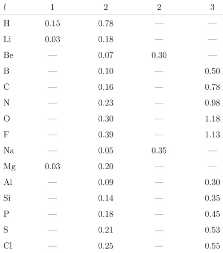
4.1.5 Recommended Exponents . . . 79
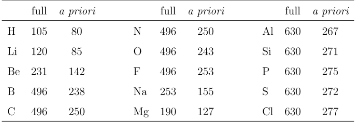
4.1.6 Efficiency of the A Priori Elimination . . . 80
4.2 Accuracy of LEDO-DFT . . . 82
4.2.1 Small Molecules . . . 83
4.2.2 Larger Molecules — Linear Alkanes . . . 87
4.2.3 Critical Cases — Assessment of the Projection Technique . 89 4.2.4 Some “Real Life” Examples . . . 90
4.3 Efficiency of LEDO-DFT . . . 96
5 Summary 99
6 Outlook 103
7 Zusammenfassung 107
B Accuracy of LEDO-DFT for a test set of 142 small molecules 117
List of Tables 125
List of Figures 127
6-31G Pople’s split-valence basis set au Hartree atomic units
AO atomic orbital
BP86 Becke–Perdew exchange-correlation functional CC2 approximate second order coupled cluster model COO canonically orthogonalized orbital
DFT density functional theory ERI electron repulsion integral
GGA generalized gradient approximation GTF Gaussian type function
HF Hartree–Fock
HOMO highest occupied molecular orbital
KS Kohn–Sham
LCAO linear combination of atomic orbitals LDA local density approximation
LEDO limited expansion of diatomic overlap LUMO lowest unoccupied molecular orbital MCSCF multi-configurational self-consistent field MO molecular orbital
MP2 second order Møller–Plesset perturbation theory PVM parallel virtual machine
RI resolution of the identity RMS root-mean-square
SCF self-consistent field STF Slater type function
SVD singular value decomposition
SVP Ahlrichs’ split-valence plus polarization basis set XC exchange-correlation
ψ(r) molecular orbital
φ(r) atomic orbital
χ(r) canonically orthogonalized orbital Ω(r) density fitting expansion function Λ(r) density fitting auxiliary function
η(r) density fitting auxiliary orbital
α, β perturbational parameters, e.g. a nuclear coordinate
ζ exponent of a basis function
Ξ(r) arbitrary charge distribution
ρ(r) and ρµν(r) electron density and overlap density φµ(r)φµ(r)
dp and dµνp expansion coefficients for electron density and overlap densities
l angular momentum quantum number
N number of AO basis functions
r position vector (x, y, z)†
r12 |r1−r2|
W,W weight operator
HKS,HKS Kohn–Sham operator
Q,Q projection operator
P first order reduced density matrix
S overlap matrix hf|gi R drf(r)g(r) hf|O|gi R dr1dr2f(r1)O(r1,r2)g(r2) (f|g) R dr1dr2f(r1)r12−1g(r2)
∆ Laplace operator, norm of a difference vector
Wpq and Vpq hΩp|W|Ωqi and (Ωp|Ωq) vii
aµν
p and bµνp hΩp|W|φµφνi and (Ωp|φµφν)
Eh, vh(r),Vh Hartree energy and potential
Exc, vxc(r),Vxc exchange-correlation energy and potential
Eext, vext(r),Vext external energy and potential
i, j indices denoting MOs or basis functions of a shell
µ, ν, κ, λ indices denoting AO basis functions or auxiliary orbitals
k, l, m, n indices denoting shells of basis functions
p, q indices denoting density fitting expansion functions
Introduction
This thesis describes the development, implementation, and benchmarking of ef-ficient algorithms for electronic structure calculations with the limited expansion of diatomic overlap density functional theory (LEDO-DFT) [1], a novel formalism in the framework of Kohn–Sham DFT (KS-DFT) [2, 3] which exhibits a favor-able scaling behavior. The general importance of quantum chemical methods, in particular of KS-DFT, and the relevance of the associated scaling behavior of the computational effort with system size are briefly sketched in this introduction followed by an outline of the contents of this work.
1.1
Background of this work
Today there is little doubt that the foundation for all of low-energy physics, chemistry and biology lies in the quantum theory of electrons and atomic nuclei. Therefore, the equations of quantum mechanics should be attempted to be solved, if such complex processes as occurring in real materials shall be described with high precision. Unfortunately, these equations are far too complicated to be solved analytically for all but the simplest (and hence most trivial) systems. The only chance to bring the power of quantum mechanics to investigations in the field of chemistry and related sciences is to solve the equations in a numerical fashion by a computational modeling of the systems of interest.
Electronic structure theory, i.e., the theoretical prediction of material proper-ties from quantum chemical methods without recourse to empirical parameters,
has advanced significantly in the recent years, serving basic science as well as applied research in numerous industries. In many fields, computer simulations have aided, stimulated, and sometimes even replaced experimental investigations. Nevertheless, many fundamental problems still continue to challenge scientists. The same complexity which precludes the exact analytical solution also results in a highly unfavorable scaling of computational effort and required resources. The computational demands of exact calculations, e.g., with the full configuration in-teraction (full CI) method, grow exponentially with the size of the system under investigation. Evidently, approximations that represent a reasonable compromise between efficiency and accuracy are needed if one desires to carry out electronic structure calculations on sizable molecules. A number of well-controlled approxi-mations which do not sacrifice the predictive power of the parameter-free nature of quantum mechanical calculations but exhibit polynomial rather than expo-nential scaling are routinely available nowadays. Among these are popular wave function based quantum chemical methods which include the effects of electron correlation in an approximate fashion such as the second order Møller–Plesset perturbation theory (MP2) and coupled cluster theory including all single, dou-ble and perturbative triple excitations (CCSD(T)). However, these correlated ab initio methods still exhibit a scaling behavior with system size of at leastO(N5).
Here, N denotes the number of basis functions employed in the calculation which in general is proportional to the number of atoms or electrons. Doubling the size of the investigated system therefore results in an increase of the required com-puting resources by a factor of at least 32, thus severely limiting the applicability of these accurate methods to large molecules.
This is where density functional theory (DFT) comes into play. The promise of DFT lies in its ability to fold into a local exchange-correlation operator the most difficult aspects of electronic structure theory. In the Kohn–Sham formula-tion of DFT, the complicated many-electron Schr¨odinger equation is replaced by an equivalent set of self-consistent one-electron equations [3]. It is precisely this feature, of treating complex many-body systems in principle exactly with only the computational expense of a self-consistent-field (SCF) calculation, which has been so appealing in KS-DFT. In the last decade electronic structure methods based on KS-DFT have evolved to a powerful quantum chemical tool and are
playing an increasing role in the ongoing effort for the determination of accurate properties of large molecular systems. Numerous electrical, magnetic, and struc-tural properties of molecules and materials have been calculated using DFT, and the extent to which DFT has contributed to the science of molecules is reflected by the 1998 Nobel Prize in Chemistry, which was awarded to Walter Kohn [4], the founding father of DFT, and John Pople [5], who was instrumental in im-plementing quantum chemical methods in computational chemistry. Nowadays, sophisticated density functionals are available in widely accessible commercial and non-commercial computer programs. Scientists applying DFT can rely on a wealth of information that has been gathered in the past and which documents the applicability and the reliability of DFT methods for molecular calculations. Especially for transition metal complexes, accuracies have been achieved that are comparable or superior to correlated wave function based theories [6–8].
A straightforward implementation of KS-DFT has anO(N4) scaling behavior.
Reduction to O(N3) is possible if density fitting is applied, i.e., if the electron
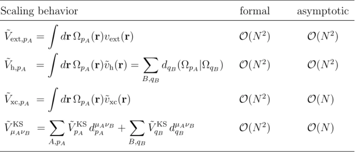
density is expanded into an auxiliary basis set. At this point it is important to distinguish between formal and asymptotic (or effective) scaling, because the actual computational cost as a function of system size is not necessarily related to the formal scaling properties. The formal scaling behavior results from a direct implementation of the equations appearing in a given formalism. However, in many cases technical tricks can be employed which exploit physical properties of the system under investigation like, e.g., that certain interactions between regions separated far enough are negligible. The prevention of the calculation of such negligible quantities can lead to a lower effective scaling behavior in the limit of large molecules which therefore is referred to as asymptotic scaling. Furthermore, a prefactor is always associated with the scaling behavior. It is clear that this prefactor will vary for different formalisms even if they share the same scaling behavior and that it will also depend on the efficiency of the algorithms used for the implementation. For sufficiently large molecular systems it is always the asymptotic scaling behavior together with the associated prefactor that determines the real cost of a calculation. The asymptotic scaling behavior for the setup of the secular matrix is O(N2) for KS-DFT, with and without
that determines the computational cost for extended systems. In the case of conventional density fitting the lower formal scaling leads to a smaller prefactor and speedups by more than a factor of 10 as compared to unapproximated KS-DFT calculations.
Recently, a novel formalism denoted as LEDO-DFT with the nice property of a formal scaling behavior as low asO(N2) for the setup of the secular matrix has
been presented by Kollmar and Hess [1]. This method therefore has the poten-tial to further reduce the prefactor associated with the asymptotic O(N2)
scal-ing of KS-DFT calculations. An implementation into the MOLPRO [9] program package demonstrates the accuracy of LEDO-DFT with respect to energetics and structural parameters for a little test set of small molecules containing H, C, N and O atoms. The authors employed a preliminary auxiliary basis set for all calcula-tions and made use of numerical gradients for the structure optimizacalcula-tions. Later, a rudimentary implementation of LEDO-DFT for single point calculations with limited features has been realized in the program package TURBOMOLE [10, 11] by the author during the course of his Diplomarbeit [12] (Master’s Thesis).
1.2
Outline of this work
This thesis builds upon the work of Kollmar and Hess [1] and extends the TUR-BOMOLE implementation mentioned above. Its main objectives have been:
1. to find a way for the systematic optimization of auxiliary basis sets 2. the optimization of auxiliary basis sets for a larger set of atom types 3. the implementation of analytical gradients for LEDO-DFT
4. the tuning of the implementation with respect to efficiency 5. the objective assessment of LEDO-DFT with respect to its
(a) accuracy and (b) computational cost
The text consists of three main parts. In chapter 2 the complete theory as necessary for a deeper understanding of all aspects of LEDO-DFT is presented. Because the process of creating a program often entails as much research as de-veloping the theory [13], chapter 3 is completely devoted to a description of the algorithms for the implementation of the formalism. In chapter 4, numerical results obtained with the implementation presented in chapter 3 are presented. First, the optimization of auxiliary orbitals for the LEDO expansion is described. Then, the accuracy and the efficiency of LEDO-DFT are critically assessed. A short overview is given at the beginning of each of these chapters to better guide the reader through the text. In chapter 5, the results obtained so far are summa-rized and some general conclusions are drawn. Finally, an outline of the direction for future work building upon this thesis is given in chapter 6.
Theory
This chapter deals with the theoretical aspects underlying the LEDO-DFT for-malism, which is intended to facilitate first-principles calculations in the frame-work of KS-DFT. Being based on the LEDO expansion, LEDO-DFT can be interpreted as a special kind of density fitting method. Therefore, after a con-cise introduction to DFT (Sec. 2.1), the main bottlenecks of DFT calculations are briefly summarized alongside with a description of established techniques to reduce their computational cost (Sec. 2.2). This is followed by a detailed re-view of density fitting methods (Sec. 2.3), actually being in wide use in DFT, which finally leads to a description of the LEDO expansion (Sec. 2.4). Next, the LEDO-DFT formalism is worked out (Sec. 2.5), followed by a presentation of the analytical gradients for the energy expression (Sec. 2.6). Finally, a projection technique to improve the SCF convergence behavior of LEDO-DFT calculations is presented in the last section of this chapter. After having presented all nec-essary ingredients, the description of the actual implementation will be given in chapter 3.
2.1
Density Functional Theory
The roots of modern density functional theory (DFT) [7, 14–22] can be traced back to the early days of quantum theory when Thomas and Fermi used models for the electronic structure of atoms which depend only on the electron den-sity [23, 24]. Later the Hartree–Fock–Slater orXα method was introduced to be
used in studies on systems with more than one atom. From todays perspective it represents one of the first density functional methods. It emerged from the work of Slater [25] who proposed to replace the complicated, non-local exchange term of the Hartree–Fock (HF) method by the approximate local exchange po-tential of Dirac [26] which is simply given byρ1/3. However, it was not until 1964 when DFT was put on a firm basis by the celebrated theorems of Hohenberg and Kohn [2], later generalized by Levy [27, 28], which state that all properties of an electronic system are functionals of the ground state electron density. In particular, the ground state energy of an electron system in an external potential, i.e., the potential due to a set of nuclei in a given arrangement, can be found by minimizing the functional of the total electronic energy with respect to variations in the density. Parr and Yang [14] have reviewed how major chemical concepts follow from the existence of such a functional. Unfortunately, it is very difficult to develop sufficiently accurate density functionals, in particular, for the kinetic energy. This is a problem that already plagued the Thomas–Fermi approach. Although the Hohenberg–Kohn theorems give a theoretically sound basis for the Thomas–Fermi approach and DFT in general, the practical importance of DFT might not have risen above that of the Thomas–Fermi model if it had not been for the ingenious idea of Kohn and Sham [3] to obtain the real, interacting elec-tronic density from an auxiliary system of hypothetical, non-interacting electrons as described below. The crucial point is that the electron density of this Kohn– Sham (KS) model system is identical to the electron density of the system of real, interacting electrons.
In KS theory [3], the total electronic energy is given as
E =Ts[ρ(r)] + Z drρ(r)vext(r) + 1 2 Z dr1dr2ρ(r1)r12−1ρ(r2) +Exc[ρ(r)], (2.1)
with r12 = |r1 −r2|. The various terms represent, in order, the kinetic energy
of the KS system (the fictitious system of non-interacting electrons), the inter-action between electrons and the external potential vext generated by the nuclei
and external fields, the Hartree energy arising from the Coulomb interactions of the electrons, and the remainder of the total energy which is referred to as the exchange-correlation (XC) energy Exc. Note that Exc, which is a crucial
to the HF wave function as in traditional ab initio methods. The electron den-sity is obtained from the KS wave function, i.e., from a reference wave function of non-interacting electrons which is simply a Slater determinant built from the eigenfunctionsψi of a single-particle Hamiltonian. For a closed-shell system one obtains ρ(r) = 2 occ. X i |ψi(r)|2, (2.2)
the sum extending over all occupied KS or molecular orbitals (MOs) ψi. An extension to the spin-polarized case is straightforward and shall not be considered here. The functional Ts representing the kinetic energy of the non-interacting
electrons is then given as
Ts[ρ(r)] = 2 occ. X i hψi| − 1 2∆|ψii. (2.3)
It must not be identified with the exact kinetic energy of the real system of interacting electrons. The important point is that it is a convenient and fairly good approximation to the exact kinetic energy based on the KS orbitals. The remainder of the exact kinetic energy is taken into account as part of the XC energy Exc.
According to the second Hohenberg–Kohn theorem [2] the ground state elec-tron density minimizesE[ρ] and hence must satisfy the Euler-Lagrange equation
δE[ρ(r)] δρ(r) = δTs[ρ(r)] δρ(r) +vext(r) +vh(r) +vxc(r) = µ. (2.4) Here, vh(r) = Z dr2r−121ρ(r2) (2.5) and vxc(r) = δExc[ρ(r)] δρ(r) , (2.6)
are the Hartree and the XC potential, respectively. The Lagrange multiplier µ
takes the constraint
Z
drρ(r) = n (2.7)
into account, where n is the number of electrons, thus guaranteeing charge con-servation. Since for Ts as explicit density functional no sufficiently accurate
therefore Eq. (2.4) cannot be solved directly, i.e., one cannot directly minimize Eq. (2.1) with respect to ρ in order to obtain the ground state energy and den-sity. Instead, this minimization is performed indirectly. For the non-interacting electrons moving in a potentialvs(r), the corresponding Euler-Lagrange equation
is
δEs[ρ(r)]
δρ(r) =
δTs[ρ(r)]
δρ(r) +vs(r) = µ. (2.8) The density solving this equation isρs. Comparing Eq. (2.8) with Eq. (2.4) shows
that both have the same solution ρ=ρs, if vs is chosen to be
vs(r) = vext(r) +vh(r) +vxc(r). (2.9)
Consequently, the density of the interacting (many-body) system in the external potential vext can be obtained by solving the one-electron Schr¨odinger equations
HKSψ
i(r) = εiψi(r) (2.10) with the KS single-particle Hamiltonian
HKS =−1
2∆ +vs(r) = − 1
2∆ +vext(r) +vh(r) +vxc(r) (2.11) and the canonical MO energies εi. Once the KS orbitals have been determined from Eq. (2.10), the total electronic energy of the real, interacting system can be obtained from Eq. (2.1).
Eq. (2.10) is somewhat deceptive, in that it looks like a simple single-particle Schr¨odinger equation. However, two features bring out the full many-body char-acter of the problem. One is that Eq. (2.10) has to be solved self-consistently since both vh and vxc depend on the electron densityρ which is a function of the
KS orbitals ψi. The other is the incomplete knowledge of the XC energy density functional Exc.
Exchange-correlation functionals
Classical electronic structure theories have always started with the exact Hamil-tonian operator, and used approximations for the wave function, usually with a single Slater determinant as a starting point. The foundation of KS-DFT begins with an approximate energy expression, the refinements placed only on the XC
term. The success of the KS method therefore hinges on the availability of good approximations toExc.
For many years the most widely used scheme has been the so-called local density approximation (LDA),
ExcLDA[ρ(r)] =
Z
drεxc(ρ(r)), (2.12)
whereεxc is the XC energy density1 in a homogeneous electron gas, known with
great accuracy from quantum Monte-Carlo calculations [29]. This approximation is obviously valid in the limit of slowly varying densities, but has proven its accuracy for a wide range of systems. The functional ELDA
xc can be divided into
exchange and correlation contributions,
ExcLDA[ρ(r)] = ExLDA[ρ(r)] +EcLDA[ρ(r)], (2.13) where the exchange contribution is given by the Dirac exchange energy func-tional [26]. A popular analytical form of the correlation contribution has been given by Vosko, Wilk and Nusair (VWN) [30], others are due to Perdew and Zunger (PZ81) [31] and Perdew and Wang (PW92) [32]. For practical purposes all LDA functionals are next to equivalent.
More recently, however, these approximations to Exc have been much
im-proved by the introduction of the generalized gradient approximation (GGA), which supplements the LDA term with one that depends explicitly on the gradi-ents of the density,
ExcGGA[ρ(r)] =
Z
drFxc(ρ(r),∇ρ(r)). (2.14)
It was the advent of GGAs that made DFT popular among chemists since these provided for the first time a level of accuracy which allows for the quantitative discussion of chemical bonds. Popular gradient corrections are the ones by Becke (B88) [33] and Perdew and Wang (PW86) [34] for the exchange contribution and the ones by Perdew (P86) [35], Becke (B88C) [36], and Lee, Yang and Parr (LYP) [37] for the correlation contribution. Perdew et al. (PW91) [38], Perdew,
1Sometimes the XC energy per particle is used instead of the XC energy density. In that case an additionalρ(r) appears under the integral on the right hand side of Eq. (2.12).
Burke and Wang (PBW96) [39] and Perdew, Burke and Ernzerhof (PBE) [40] have given widely used expressions for the complete XC energy. Many other GGA functionals are available, and new ones continue to appear. Some of these approximate functionals were constructed in a semiempirical fashion with many parameters fitted to chemical data, others were constructed to incorporate key properties of the exact XC energy. The latter functionals usually perform well for both small and extended systems. While the semiempirical functionals can achieve remarkably high accuracy for atoms and molecules, they are typically less accurate for surfaces and solids [41].
The most widespread functional among chemists is probably the one called B3LYP [42]. It is a so-called hybrid functional meaning that some portion of exact exchange, i.e. non-local HF-like exchange expressed with KS orbitals, is mixed into the expression of the XC energy as introduced by Becke [43]. Another beyond-GGA development is the emergence of so-called meta-GGAs, which de-pend, in addition to the density and its derivatives, also on the Laplacian of the density or the KS kinetic energy density [44, 45]. These functionals have given favorable results even when compared to the best GGAs [41, 46, 47], but the full potential of this type of approximation has not yet been explored sys-tematically. Finally, it should be mentioned that in the framework of orbital dependent density functionals, an exact treatment of the exchange contribution is feasible [48]. Future developments will be aimed at a description of correlation effects compatible to exact exchange (hyper-GGAs) [47, 49].
Basis set methods
Although in principle the MOs can be represented on a grid and the KS equations solved numerically, in molecular calculations the MOs are in general expanded into a set {φµ}of atom-centered basis functions or atomic orbitals (AOs) accord-ing to
ψi(r) =
X
µ
Within this linear combination of atomic orbitals (LCAO) expansion the electron density [Eq. (2.2)] is then given as
ρ(r) =X µ,ν
Pµνφµ(r)φν(r), (2.16) whereP is the first order reduced density matrix with elements
Pµν = 2
occ.
X
i
CµiCνi. (2.17)
The expression for the total electronic energy [Eq. (2.1)] now reads as
E =X µ,ν Pµνhφµ| − 1 2∆ +vext|φνi+ 1 2 X µ,ν,κ,λ PµνPκλ(φµφν|φκφλ) +Exc[ρ(r)]. (2.18)
In Eq. (2.18) the charge density notation for the electron repulsion integrals (ERIs),
(φµφν|φκφλ) =
Z
dr1dr2φµ(r1)φν(r1)r12−1φκ(r2)φλ(r2), (2.19)
has been employed. The variational parameters in this energy expression are the MO coefficients or the elements of the density matrix and application of the variational principle leads to the matrix eigenvalue equation
HKSC=SCε (2.20)
instead of the operator equation (2.10). In Eq. (2.20) HKS is the matrix
repre-sentation of the KS operator (2.11) in the AO basis,
HµνKS =hφµ|HKS|φνi, (2.21)
S is the overlap matrix with elementsSµν =hφµ|φνi, and the matrix Ccontains as elements Cµi the MO coefficients Cµi which are obtained by solving the KS equation (2.20). The matrixε of the Lagrange multipliers for the orthonormality constraints is a diagonal matrix which can be identified with the KS matrix in the canonical MO basis and its diagonal elements represent the corresponding MO energies εi of the KS orbitals ψi.
Due to decades of experience with HF calculations much is known about the construction of basis functions φµ that are suitable for molecules. Almost all of
this continues to hold in DFT, a fact that has greatly contributed to the pop-ularity of DFT in chemistry. The most popular types of basis functions φµ for molecular calculations can be classified with respect to their behavior as a func-tion of the radial coordinate into Slater type funcfunc-tions (STFs) [50], which decay exponentially from their origin, and Gaussian type functions (GTFs) [51], which have a Gaussian behavior. While STFs more closely resemble the true behavior of atomic wave functions, GTFs are much easier to handle numerically. In partic-ular an analytical evaluation of the ERIs is possible in an efficient manner. This is the reason for the predominance of GTFs not only in conventional ab initio
methods but also in programs for molecular DFT calculations [52].
2.2
Computational Aspects of DFT
Calcula-tions
In general, there are three important bottlenecks in Gaussian-based KS-DFT calculations. These are the evaluation of the Hartree energy, the XC quadrature and the diagonalization of the KS Hamiltonian. In this section, a short description of these bottlenecks along with a summary of existing techniques to speed up the respective part of the calculations shall be given, before density fitting methods are discussed thoroughly in the subsequent section.
Evaluation of the Hartree energy
In Gaussian-based KS theory the Hartree energy
Eh= 1 2(ρ|ρ) = 1 2 X µ,ν,κ,λ PµνPκλ(φµφν|φκφλ) (2.22) and the corresponding contributions to the KS matrix, i.e. the matrix elements of the Hartree potential (frequently termed Coulomb matrix)
Vh,µν = ∂Eh ∂Pµν =X κ,λ Pκλ(φµφν|φκφλ) = (φµφν|ρ) (2.23) have to be computed from four-index ERIs. Formally, this is an O(N4)
limit of extended systems scales asO(N2) if appropriate prescreening of the ERIs
is employed [53–56]. However, despite huge advances in integral evaluation tech-niques [57–72], the prefactor for this quadratic scaling is large enough to make the evaluation of the ERIs the rate-limiting step even for moderate-sized systems. As a consequence a wide range of refined technical tricks and elegant approximations have been devised to reduce the effective scaling and enable the rapid evaluation of the Hartree energy and the matrix elements of the Hartree potential.
Ahmadi and Alml¨of have developed an algorithm for the evaluation of the Coulomb matrix in which the density matrix is summed into the underlying Gaussian integral formulas with substantial benefits in the floating point oper-ation (FLOP) cost [73]. The “J matrix engine” [74–76] from Head-Gordon et al. and the Quantum Chemical Tree Code (QCTC) [77] work in a similar fash-ion. The latter is a modified version of the McMurchie/Davidson [61] algorithm for the ERI evaluation which is based upon a representation of the density in a Hermite Gaussian type function (HGTF) basis and has been reported to lead to sub-O(N2) scalings [77]. All of these algorithms do not require any
approx-imations. For a review about fast methods for computing the Coulomb matrix in a basis of GTFs up to the year 1996 the reader is referred to reference [78]. An evaluation of the Coulomb potential on an integration grid by explicit use of the Poisson equation has also been explored, but it does not lead to competitive methods [79].
Other research efforts have focused on methods that provide approximations to the ERIs. The Fourier transform Coulomb (FTC) method [80] is based on an intermediate discrete Fourier transformation of the electron density. It is in some sense similar to the Gaussian and augmented plane-wave (GAPW) method [81] and was shown to exhibit near-linear asymptotic scaling while retaining high nu-merical accuracy. Important progress with respect to the Coulomb problem has been achieved by generalization of the fast multipole method (FMM) [82, 83] to Gaussian charge distributions, which leads to linear scaling for the asymp-totic limit of very large systems [84–89]. In this method the computation of the Coulomb interaction is divided into a near-field and a far-field part, the latter of which is treated by accurate multipole approximations and the former by exact analytical integration. The recursive bisection method (RBM) [90] works in a
similar fashion and exhibits the same asymptotic scaling behavior. The linear scaling KWIK/CASE algorithm [91–96] relies on a similar partitioning, but the long-range part is computed by Fourier summations.
In practice, however, much of the computational effort for molecules of chem-ical interest does not fall into the asymptotic regime, and the underlying formal scaling behavior which determines the prefactor has a significant quantitative ef-fect on performance. The analytical integration of the four-index ERIs is still an expensive part of the calculation, and efficient algorithms are required to achieve high computational throughput. Fitting procedures for the electron density are widely used in DFT calculations to avoid the unfavorable formal O(N4) scaling
behavior in the processing of the ERIs and shall be reviewed in detail in Sec. 2.3. The pseudospectral approximation [97–101] is a different approach in a sim-ilar spirit. This method uses a grid as an auxiliary basis to expand the electron density (or the potential from it), which leads to the same formal O(N3)
scal-ing behavior as conventional density fittscal-ing procedures. It should be mentioned that density fitting has already been successfully employed for the evaluation of the nearfield interactions in order to reduce the prefactor of the fast multipole method [102].
If hybrid DFT functionals are used, the HF-like (orbital) exchange energy has to be evaluated from four-index ERIs like the Hartree energy. However, for non-metallic systems with a large HOMO-LUMO gap the density matrix is decaying exponentially [103]. This has lead to the development ofO(N) methods like ONX [104–106], LinK [107] and others [108] which exploit the fast decaying nature of the exchange interaction.
Exchange-correlation quadrature
The XC energy Exc in DFT is given by Eq. (2.14). As indicated in this formula,
the XC functional Fxc can depend both on the electron density ρand its gradient ∇ρ. In general this dependence is very complicated and the XC integrals cannot be solved analytically, even if the density is expressed in a basis of Gaussian charge distributions [Eq. (2.16)]. Instead, they are evaluated using an integration grid.
This is a set of pointsrj = (xj, yj, zj)† and non-negative weights ωj such that
Z
drf(r)≈X
j
ωjf(rj). (2.24)
The XC energy which is actually computed is thus given by
ExcGGA =X j
ωjFxc(ρ(rj),∇ρ(rj)). (2.25) The integrand is usually partitioned over atomic points using a weight scheme [109, 110], and a further decomposition into radial and angular com-ponents of each atomic contribution is introduced [111–113]. The formal scaling for the setup of an integration grid with such a weight scheme is O(N3). Other
steps in the numerical quadrature also yield O(N3) scaling simply because the
number of atomic-based grid points grows linearly with molecular size and their contributions need to be evaluated over every pair φµφν of AO basis functions. Advantages of such a numerical integration are the possibility to control and systematically enhance the numerical accuracy and the insensitivity of the in-tegration itself to the type of density functional in use. The numerical XC quadrature has long been recognized as being intrinsically linear scaling due to the fast decaying nature of the basis functions used [114, 115]. Much attention has also been focused on the construction of the grid with respect to the effi-ciency of the resulting code and linear scaling quadrature grid construction is feasible [116].
Diagonalization
The matrix eigenvalue equation (2.20) is usually solved by diagonalization of the KS matrix. Today, it turns out that the diagonalization steps which scale as
O(N3) are becoming more and more important, although the prefactor is very
small. This is partly because it is almost trivial to make use of parallel process-ing when constructprocess-ing the Kohn–Sham matrix, while this is more difficult when diagonalizing. As a result, there are methods available to replace the diagonal-ization step by procedures with a more favorable scaling behavior, like conjugate gradient [117–120] or quasi Newton approaches [121, 122].
2.3
Review of Density Fitting Methods
In this section, density fitting methods shall be reviewed. It has already been mentioned that these are widely used in DFT. Implementations are documented for the programs DGauss [123], DeFT [124], ParaGauss [125], ADF [126], Turbo-mole [127], Molpro [128], Orca [129] and Magic [130] and are most likely available in virtually any other KS-DFT program, even if not explicitly documented in the scientific literature. Furthermore, density fitting procedures have been success-fully applied as integral approximations in the framework of HF calculations [131– 136] for both the Coulomb problem and the HF exchange. Density fitting has also proven to offer significant advantages for multi-configurational SCF (MC-SCF) [132, 137], second order Møller–Plesset perturbation theory (MP2) [138– 142], CC2 [143, 144], coupled cluster [145, 146] and, more recently, explicitly correlated MP2-R12 [147–149] calculations.
2.3.1
Fit of an Arbitrary Charge Distribution
Consider an arbitrary charge distribution Ξ(r). Suppose that a model distribution
˜
Ξ(r) = X p
Ωp(r)dp =Ω†d (2.26)
shall be formed by expanding this charge distribution into a set {Ωp}of auxiliary functions. d is the coefficient vector that minimizes the norm of the difference vector Ξ−Ξ between the exact and the approximated charge distribution. Several˜ choices are possible for defining this norm, generally having the form
∆(W) = Z dr1dr2 h Ξ(r1)−Ξ(˜ r1) i W(r1,r2) h Ξ(r2)−Ξ(˜ r2) i =hΞ|W|Ξi −2hΞ˜|W|Ξi+hΞ˜|W|Ξ˜i. (2.27)
W is the weight operator whose Fourier transform has to be positive [150]. This norm is minimized with respect to the coefficients dp by setting ∇d∆(W) = 0 resulting in the system of linear equations
X
q
for the determination of the expansion coefficients dp. This can be rewritten in matrix notation as
Wd=a (2.29)
with the solution
d=W−1a, (2.30)
where Wpq =hΩp|W|Ωqi and ap =hΩp|W|Ξi. The matrix W is strictly positive definite if the expansion functions Ωp are linearly independent which guarantees the mathematical existence of the solution (2.30). Any prescribed accuracy in fitting the charge distribution Ξ(r) can thus be achieved if the expansion basis is sufficiently flexible and approaches completeness. Additional constraints, e.g. such that the total charge of Ξ(r) is exactly reproduced, can be easily imposed by the use of Lagrangian multipliers. In the following, however, this option shall not be considered. The approximated charge distribution is then given as
˜
Ξ(r) =Ω†d=Ω†W−1a. (2.31) The generalized least squares fitting procedure described here can also be inter-preted as a projection of the charge distribution Ξ(r) onto a basis{Ω0p} orthonor-mal in the linear vector space with metric W which is obtained by symmetric orthonormalization [151] as
Ω0 =W−1/2Ω. (2.32)
The projection becomes ˜
Ξ(r) = X p
|Ω0pihΩ0p|W|Ξi=Ω0†hΩ0|W|Ξi=Ω†W−1a, (2.33) in analogy with Eq. (2.31).
In the context of DFT, the charge distribution that shall be approximated is the electron density ρ(r) in order to facilitate the evaluation of the Hartree energy [Eq. (2.22)]. For doing so, the choice of the weight operator W is very important. UsingW =δ(r12) [152–154] amounts to minimizing the least-squares
error in the charge distribution2,
∆(W =δ(r12)) =
Z
dr|Ξ(r)−Ξ(˜ r)|2. (2.34)
At first sight, this seems very attractive since the integralsWpq andap involved in the fitting process reduce to simple overlap integrals. However, it was found that approaches usingW =r12−1are at least an order of magnitude more accurate [155– 157]. These approaches minimize the least squares error of the electric field because [155]
∆(W =r−121) = (Ξ−Ξ˜|Ξ−Ξ) =˜ 1 4π
Z
dr|E(r)−E˜(r)|2, (2.35) whereE and ˜Eare the electric fields arising from the exact and the fitted charge distribution. Expression (2.35) is frequently denoted as Coulomb norm. This form of fitting has also been suggested by Billingsley and Bloor [158], Whit-ten [159] and Fortunelli and Salvetti [160] for the approximation of overlap densities, by Hall for point charge models [161] and molecular electron densi-ties [162, 163], and is in wide use nowadays. It has not yet been established whether the idea of minimizing the least squares error in the Hartree potential
vh of the charge distribution,
∆(W =−r12) =
Z
dr|vh(r)−˜vh(r)|2, (2.36)
by using the weight operator W =−r12 [164], offers any advantage.
2.3.2
Fit of the Complete Electron Density
All current DFT implementations exploiting density fits rely on the expansion of the complete electron density, Eq. (2.16), according to
˜
ρ(r) =X p
Ωp(r)dp =Ω†d (2.37)
into a set {Ωp} of atom-centered auxiliary functions. This is desirable because the AO product basis {φµφν} in which the exact electron density is expanded is nearly linear dependent and grows as O(N2) whereas the dimension of the basis {Ωp} increases only as O(N). As described above, the expansion coefficients are obtained from the system of linear equations
with the solution
d=W−1a. (2.39)
The elementsap of the inhomogeneity vector are now defined as
ap =hΩp|W|ρi=
X
µ,ν
aµνp Pµν, (2.40)
with the three-index integrals
aµνp =hΩp|W|φµφνi. (2.41) The Hartree energy, given by Eq. (2.22), is then approximated as
˜ Eh = 1 2( ˜ρ|ρ˜) = 1 2d †Vd, (2.42) where Vpq = (Ωp|Ωq) (2.43)
is a two-index ERI. An analysis of the error
Eh−E˜h =
1
2{(ρ|ρ)−( ˜ρ|ρ˜)}= 1
2{(ρ−ρ˜|ρ−ρ˜) + 2(ρ−ρ˜|ρ˜)} (2.44) between the exact and the fitted Hartree energy shows that it contains terms linear and quadratic in the fitting errorρ−ρ˜in the electron density. The form of Eq. (2.44) therefore suggests the alternative approximation
˜ Ehrob = (ρ|ρ˜)− 1 2( ˜ρ|ρ˜) = b † d−1 2d † Vd (2.45)
which goes back to Dunlapet al. [155] In Eq. (2.45) the elements of the vectorb
are defined as
bp = (Ωp|ρ) =
X
µ,ν
bµνp Pµν (2.46)
with the three-index ERIs
bµνp = (Ωp|φµφν). (2.47) Fitting expressions of this kind are called robust since the error
Eh−E˜hrob =
1
2{(ρ|ρ)−2(ρ|ρ˜) + ( ˜ρ|ρ˜)}= 1
is always quadratic in the fitting errorρ−ρ˜. The robust energy expression (2.45) is also variational because it is a lower bound to the exact Hartree energy,
˜
Ehrob ≤Eh, (2.49)
which follows directly from Eq. (2.48). In other words, the expansion coefficients
dp have been determined in such a way as to maximize the robust approximation to the Hartree energy. Therefore, derivatives of the expansion coefficients will not appear in expressions for the gradient of the energy if robust fitting is per-formed. The concepts of robust and variational fitting in various contexts have been thoroughly discussed by Dunlap [155, 165–172].
For a generally fitted case one obtains ˜ Vh,µν = ∂E˜h ∂Pµν = ∂ ∂Pµν 1 2d † Vd= ∂d† ∂Pµν Vd (2.50)
for the matrix elements of the Hartree potential and the derivatives of the fitting coefficients are required. These are given as
∂d
∂Pµν
=W−1 ∂a
∂Pµν
=W−1aµν, (2.51)
which follows from Eqs. (2.39) and (2.40). The approximated matrix elements of the Hartree potential thus become
˜
Vh,µν =aµν †
W−1Vd. (2.52)
For robust fitting the approximated matrix elements are given as ˜ Vhrob,µν = ∂ ˜ Erob h ∂Pµν =bµν†d+aµν†W−1{b−Vd}. (2.53) It is not possible to say much about the quality of the fitted matrix elements ˜Vh,µν given by Eq. (2.52). For the robust approximation ˜Vrob
h,µν [Eq. (2.53)], however, the first term on the right hand side is (φµφν|ρ˜) and the term in the brackets is (Ω|ρ−ρ˜). Thus, the approximation of the matrix elements will be good, if the fit for the electron density is sufficiently accurate.
If the Coulomb norm Eq. (2.35) is employed in the fitting procedure, then
W =V and a=b and the expansion coefficients are obtained from the system of linear equations
with the solution
d=V−1b. (2.55)
The elements of V are two-index ERIs as defined in Eq. (2.43) and b contains three-index ERIs [Eqs. (2.46) and (2.47)].
Now the following equality holds [cf. Eq. (2.54)],
( ˜ρ|ρ˜) = d†Vd =b†d= (ρ|ρ˜). (2.56) Thus the linear term in the error of the fitted Hartree energy [Eq. (2.44)] vanishes and the robust and the simple approximation to the Hartree energy become identical, ˜ Ehrob = ˜Eh = 1 2d † Vd. (2.57)
This explains the observation that the Coulomb norm is the best. The derivatives of the fitting coefficients with respect to the elements of the density matrix are in this case given as
∂d
∂Pµν
=V−1bµν (2.58)
and the approximated matrix elements of the Hartree potential become ˜ Vh,µν = ∂d† ∂Pµν Vd=bµν†d = (φµφν|ρ˜). (2.59) This expression is of course identical to the robust approximation and the error in the matrix elements will be small if the fit of the electron density is good.
Scaling behavior
Before discussing methods fitting individual overlap densities, some conclusions about the scaling behavior of methods fitting the complete electron density shall be drawn. For simplicity, it will be assumed that the Coulomb norm has been employed. The formal scaling behavior is O(N3) for the evaluation of the ERIs
since only two- and three-index quantities Vpq and bµνp have to be evaluated. Due to the long-range nature of the Coulomb interaction the asymptotic scal-ing behavior remains O(N2) like for the four-index ERIs, however with a much
smaller prefactor. The number of ERIs that need to be explicitly evaluated is much smaller because the number of required fitting functions Ωp is considerably
smaller than the number of significant overlap densitiesφµφν generated from the AO basis set. A speed-up by more than a factor of 10 is generally achieved and the computational expense is typically dominated by the numerical quadrature for the evaluation of the XC energy and its matrix elements [127]. The necessity to compute at most three-center ERIs is furthermore very appealing since these can be evaluated with a much simpler algorithm than for the general case [173]. The determination of the expansion coefficients requires the inversion of the ma-trix V whose dimension grows linearly with the system size. The computational effort for such a matrix inversion grows cubically with the dimension of the ma-trix. Although the prefactor is rather small, the O(N3) scaling of this matrix inversion might therefore become dominant for very large systems. The actual determination of the expansion coefficients from Eq. (2.55) is done in O(N2)
operations in each SCF iteration.
There have also been efforts to restrict the fit basis in such density fitting methods. They are based on a partitioning of the total electron density into con-tributions from different regions in space. The approach of Baerends et al. [153] relies on the decomposition into atom pair densities according to
ρ(r) = X A≥B (2−δAB)ρAB(r), (2.60) with ρAB(r) = X µA,νB PµAνBφµA(r)φνB(r). (2.61) The additional subscript (A, B) indicates the particular atom on which an AO is located. Each of these atom pair densities is fitted individually using only fit functions located on the respective atoms A and B. Thus, the fitting procedure requires O(N2) inversions of matrices V
[AB] of size-independent dimension. At
the same time the integrals of the inhomogeneity of the system of linear equations (2.54) for the determination of the expansion coefficients reduce to two-center in-tegrals of the type bµAνB
pA = (ΩpA|φµAφνB). The resulting formal O(N
2) scaling
for the fitting procedure reduces to linear scaling in the asymptotic regime be-cause the number of significant atom pair densities is O(N) [126, 174]. For the evaluation of the approximated matrix elements ˜Vh,µν of the Hartree potential according to Eq. (2.59), however, three-index ERIs bµν
required. This yields a formal O(N3) scaling behavior for the evaluation of the
ERIs which reduces toO(N2) in the asymptotic limit, just as for methods fitting
the complete electron density. If the matrix elements of the Hartree potential are evaluated by numerical quadrature, as is actually done in the work of Baerendset al.[153], then the Hartree potential has to be first evaluated at each grid point. This is a formalO(N2) process because the number of fitting functions scales
lin-early as in the worst case does the number of sampling points for the potential. Because the Coulomb interaction is long range, this scaling behavior cannot be reduced by simple cut-off schemes [126, 174]. The subsequent evaluation of the matrix elements is a formalO(N3) process which can be reduced toO(N) in the asymptotic limit by employing cut-off techniques similar to the ones used for the XC quadrature. The density fitting procedure can also be implemented inO(N) versions by employing a divide-and-conquer (DAC) approach for the partitioning of the electron density [175–179]. The formal and asymptotic scaling behavior for the evaluation of the matrix elements of the Hartree potential, however, remains in any caseO(N3) andO(N2), respectively. Note that simple fitting expressions which work with a different expansion basis for different parts of a subdivided electron density are neither robust nor variational. It should finally be mentioned that a subdivision of the electron density enables a trivial parallelization of the density fitting process.
Auxiliary basis sets for the density expansion
The choice of an auxiliary basis for the expansion of the electron density is cer-tainly a topic that requires extensive and lengthy experimentation. However, in order to reproduce SCF total energies with good accuracy, it has been shown that the reproduction of the behavior of the exact expansion near the atomic nuclei is important [157]. Therefore, the expansion basis set should include one-center products of the AO basis set, which account for by far the largest contributions to the total electron density. Consequently, the auxiliary functions should cover the range of the sums of the exponents and angular momentum quantum numbers of the original basis functions. In practice, it is sufficient to use a relatively short, even-tempered expansion ranging between the highest and lowest exponent given by this recipe [180–182]. Efficient and at the same time accurate auxiliary basis
sets for the density expansion are available [127, 183]. The exponents of these basis sets fulfill a dependence similar to the definition of an even-tempered basis and have been optimized by exploiting the variational property of the approx-imated energy expression, Eq. (2.49). An increase of computational efficiency has recently been achieved by the substitution of a large part of the expansion functions by so-called Poisson functions. Although in this case the total number of expansion functions required for the density fit increases, the major part of the ERIs become simple overlap integrals without further approximation [128, 184].
2.3.3
Fit of Overlap Densities
The most general approach to the fit of individual overlap densities φµφν ≡ρµν was suggested by Vahtras et al. [157]. In contrast to the projection of diatomic differential overlap (PDDO) approach by Newton [152] and the limited expan-sion of diatomic overlap (LEDO) approach by Billingsley and Bloor [158], their method uses the same fit basis{Ωp}of atom-centered expansion functions for all overlap densities to be fitted. In analogy to Eq. (2.37) for the expansion of the complete electron density, the expansion of individual overlap densities can thus be written as ρµν(r)≈ρ˜µν(r) = X p Ωp(r)dµνp =Ω † dµν. (2.62)
For the sake of simplicity it will be assumed in the following that the Coulomb norm [Eq. (2.35)] is used for the definition of the scalar product. Then the expansion coefficients dµν
p are obtained from the system of linear equations
Vdµν =bµν (2.63)
with solution
dµν =V−1bµν, (2.64)
where Vpq = (Ωp|Ωq) and bµνp = (Ωp|ρµν) are two- and three-index ERIs, similar to Eqs. (2.54) and (2.55) for the fit of the complete electron density. Taking the symmetry of the matrix V into account, any four-index ERI can thus be approximated as
(ρµν|ρκλ)≈( ˜ρµν|ρ˜κλ) =dµν †
Incidentally, the same expression is obtained if a conventional resolution of the identity (RI) is introduced into the ERIs,
1 = ∞ X p,q |ΩpiVpq−1hΩq| ≈ X p,q |ΩpiVpq−1hΩq|, (2.66) where the approximate equality reflects the incompleteness of the expansion ba-sis. Therefore, density fitting is frequently denoted as RI approximation by some authors. As a matter of fact, this approximation is an inner projection similar to the method of Beebe and Linderberg which is based on the Cholesky decomposi-tion of the ERI matrix [185, 186]. Here, however, the projecdecomposi-tion is formulated in terms of an auxiliary set of basis functions{Ωp}, rather than to generate the pro-jection manifold explicitly from the original overlap densities. Note, that density fitting mathematically resembles a (truncated) RI only in the specific case where the weight operatorW used in the metric of the expansion basis is the same as in the target integral. Furthermore, RIs do not offer a framework in which to discuss fitting criteria, constraints or robust fitting.
An analysis of the error
(ρµν|ρκλ)−( ˜ρµν|ρ˜κλ) = (ρµν−ρ˜µν|ρκλ−ρ˜κλ) + (ρµν−ρ˜µν|ρ˜κλ) + ( ˜ρµν|ρκλ−ρ˜κλ) (2.67) between the exact and the approximate ERIs shows that it contains terms linear and quadratic in the fitting error ρµν−ρ˜µν. However, if the Coulomb norm has been employed, the expansion coefficients are obtained from Eq. (2.64) and the following equality holds,
( ˜ρµν|ρ˜κλ) =dµν † Vdκλ =bµν†dκλ = (ρµν|ρ˜κλ) =dµν†bκλ = ( ˜ρµν|ρκλ). (2.68)
Thus the linear error terms in Eq. (2.67) vanish and the approximation is robust. It is important to realize that this holds only if the Coulomb norm has been employed.
Insertion of the expansion for the overlap densities [Eq. (2.62)] into the ex-pression for the electron density [Eq. (2.16)] yields
˜
ρ(r) = X p
for the approximate electron density. This expression is identical to Eq. (2.37) for the fit of the total electron density. Here, however, the expansion coefficients
dp for the electron density have been obtained by contraction of the elements of the density matrixP with the expansion coefficientsdµνp for the overlap densities according to
dp =
X
µ,ν
dµνp Pµν. (2.70)
In analogy to Eq. (2.46), a vector b with components
bp = (Ωp|ρ) =
X
µ,ν
bµνp Pµν (2.71)
can be defined. Similar relations as derived for the fit of the complete electron density also hold for the fit of individual overlap densities. Specifically, the ap-proximated Hartree energy is given as
˜ Eh = 1 2( ˜ρ|ρ˜) = 1 2d † Vd, (2.72)
and the approximated matrix elements of the Hartree potential are given as ˜ Vh,µν = ∂E˜h ∂Pµν = ∂d† ∂Pµν Vd =dµν†Vd= ( ˜ρµν|ρ˜). (2.73) The derivatives of the expansion coefficients dp with respect to the elements Pµν of the density matrix yield the expansion coefficientsdµνp for the overlap densities
ρµν, as can be seen from Eq. (2.70). While these need not be explicitly determined in methods fitting the complete electron density, a comparison of Eqs. (2.58) and (2.64) shows, that also in that case they do appear implicitly in the expression for the approximated matrix elements of the Hartree potential. Using Eqs. (2.63), (2.70) and (2.71), Eqs. (2.72) and (2.73) can be rewritten as
˜ Eh = 1 2b † d= 1 2(ρ|ρ˜) (2.74) and ˜ Vh,µν =bµν † d= (ρµν|ρ˜). (2.75)
It is very important to note that the step leading from Eqs. (2.72) and (2.73) to Eqs. (2.74) and (2.75) can only be performed if
a) the fit basis {Ωp} is identical for all overlap densities ρµν and
b) the Coulomb norm [Eq. (2.35)] has been employed for the fitting procedure. Only in this case the simple approximation of the ERIs and thus of the Hartree energy is identical to the robust expression. Note that the approximated ERIs are not a bound to the exact ERIs, i.e. they can be smaller or larger in magnitude. The approximated Hartree energy, however, is a lower bound to the exact Hartree energy, just as in methods fitting the complete electron density.
Requirements to the expansion basis
Now it is possible to draw an interesting conclusion. As a fit for each individual overlap density ρµν is performed, one might expect from Eq. (2.73) that the fit basis has to be sufficiently large to reproduce any particular member of the set of overlap densities with good accuracy. However, this is not the case as becomes evident by comparing Eqs. (2.23), (2.73) and (2.75). It can be easily seen that the matrix elements Vh,µν of the Hartree potential are well approximated if a good fit for the total electron density is obtained, i.e. if ρ and ˜ρ are sufficiently close. According to Eqs. (2.69) and (2.70), it is sufficient for the representation of the complete electron density to determine expansion coefficientsdµνp corresponding to density matrix elements Pµν of significant magnitude. It is obvious that the fit of the total electron density is a much easier task than the fit of each overlap density generated by the AO basis functions, thus requiring a much smaller fit basis. The most extreme example is perhaps a closed-shell atom which has a spherically symmetric electron density. Hence, s-type functions are sufficient for a density fit. It has been found that even electron densities of molecules can be fitted quite accurately by short expansions of spherical Gaussians located on the nuclei [162]. Clearly, this would be an extremely poor basis for a fit of individual AO products. However, it is sufficient for a good approximation of the matrix elements of the two-electron Coulomb part of such products. It should be noted that the demand on the expansion basis may be a lot higher in other types of calculations, where products that have nothing to do with the density expansion must also be accurately represented. This is the case, e.g., if density fitting is employed for the HF exchange (without reducing the formal
scaling behavior), which requires products φµψi between AO basis functions and occupied MOs to be fitted. In the case of MP2 calculations, products of the type
ψiψa between occupied and virtual MOs have to be fitted. Ten-no and Iwata successfully employed one-center AO products φµ0Aφµ00A as auxiliary functions in HF and MCSCF calculations [132, 137] and optimized auxiliary basis sets are available both for HF [135] and MP2 [140, 141, 144] calculations.
Scaling behavior
Although the approach of Vahtras et al., just like methods fitting the complete electron density, is not very demanding with respect to the fit basis, it has a rather unfavorable formal scaling behavior. The number of overlap densities ρµν grows as O(N2) with the system size. For each of these overlap densities the system of linear equations (2.63) has to be solved. Since the dimension of the fit basis also grows linearly with the system size, the numerical effort for obtaining the expansion coefficients for a particular overlap density scales as O(N2), once
the matrixV has been inverted. Altogether, one therefore ends up with the same formalO(N4) scaling just as the unapproximated method. However, the prefactor
might be rather favorable and, in contrast to methods fitting the total electron density, the fit does not have to be repeated in every SCF cycle. It is clear, that the fit has to be performed only for productsφµφν of AOs with significant overlap, the number of which is of O(N) in the limit of large molecules. Therefore, the asymptotic scaling for the fitting process is O(N3) due to the matrix inversion
like for the fit of the complete electron density.
2.3.4
Fit of Overlap Densities with a Restricted
Expan-sion Basis
It seems desirable to avoid the increase of the fit basis with system size for the fit of individual overlap densities which would lead to formalO(N2) scaling. Indeed, the success of the expansion technique for diatomic systems suggests [182] that it is sufficient to use a local expansion in Eq. (2.62), i.e., to use a sparse (blocked) set of expansion coefficients{dµν
p }, with coefficients only for the expansion functions Ωp on the two centers where φµ and φν are centered. Such an expansion for
diatomic overlap densities φµAφνB ≡ ρµAνB given by a product of AOs centered on atoms A and B can be written as
φµA(r)φνB(r)≈ X pA ΩpA(r)d µAνB pA + X qB ΩqB(r)d µAνB qB , (2.76)
or, in a shorthand notation, as
ρµAνB ≈ρ˜µAνB =Ω † Ad µAνB A +Ω † Bd µAνB B =Ω † [AB]d µAνB [AB] . (2.77)
Note that the caseA =B is assumed to be handled in analogy to Eq. (2.76) as
φµ0A(r)φµ00A(r)≈ X pA ΩpA(r)d µ0Aµ00A pA . (2.78)
The expansion functions {Ωp} are restricted to be located on atoms A and B. Indeed it is not obvious that an expansion function located on an atom C far away from atomsAand B should improve the fit significantly. Furthermore, the possible benefit in fitting diatomic overlap densities ρµAνB obtained by including expansion functions from other atoms C 6= A, B is heavily system dependent. Since the presence of atomsC close to ρµAνB is accidental, the quality of the fit could vary from one system to another depending on the accidental surrounding of a pairAB by other atoms. A reliable expansion basis will have to be able to fit an overlap density ρµAνB accurately, with approximately the same precision, under all circumstances, also in cases where other atoms are remote or not present at all, for instance in the diatomic molecule AB. A restriction of the expansion basis like in Eq. (2.76) makes the quality of the fit independent of the molecular environment.
In analogy to Eq. (2.54) for the fit of the complete electron densityρand Eq. (2.63) for the fit of individual overlap densities ρµν, the expansion coefficients
dµAνB
pA and d
µAνB
qB are obtained from the system of linear equations
VAAdµAνB A +VABd µAνB B =b µAνB A VBAdµAνB A +VBBd µAνB B =b µAνB B (2.79)
if the Coulomb norm [Eq. (2.35)] is employed, i.e. forW =r12−1. The definition of the matrixVand the vectorbµAνB is the same as for the fit of individual overlap densities ρµν, i.e. VpAqB = (ΩpA|ΩqB) and b
µAνB
Eqs. (2.63) and (2.79) shows that the latter involves certain blocks of the complete matrix V depending on the location of the AOs forming the overlap densities to be fitted. To put it in more mathematical terms, the overlap densities are now projected onto subspaces of the total space spanned by the expansion basis{Ωp}. These subspaces can differ for different overlap densities. Of course it is also possible to use distinct sets {ΩAB
pA } of expansion functions on an atom A for different atom pairs AB containing that atom depending on e.g. the type of the partner atomB or the interatomic distance. The system of linear equations (2.79) can be rewritten as V[AB]dµAνB [AB] =b µAνB [AB] (2.80) with solution dµAνB [AB] =V −1 [AB]b µAνB [AB] , (2.81) where V[AB]= VAA VAB VBA VBB , (2.82) dµAνB [AB] = dµAνB A dµAνB B (2.83) and bµAνB [AB] = bµAνB A bµAνB B (2.84)
Introducing the notation
V[ABCD]= VAC VAD VBC VBD , (2.85)
any four-center ERI can be approximated as (ρµAνB|ρκCλD)≈( ˜ρµAνB|ρ˜κCλD) =d
µAνB†
[AB] V[ABCD]d
κCλD
[CD] . (2.86)
The error between the exact and the approximated ERIs,
(ρµAνB|ρκCλD)−( ˜ρµAνB|ρ˜κCλD) = (ρµAνB −ρ˜µAνB|ρκCλD −ρ˜κCλD)
contains terms that are linear and quadratic in the fitting error ρµAνB −ρ˜µAνB. It is important to realize that even if the Coulomb norm has been employed, the linear error terms do not vanish for the general case of four-index ERIs because the expansion basis differs for each atom pair. In order to get rid of the linear error terms, the robust approximation
( ˜ρµAνB|ρ˜κCλD) rob = (ρ µAνB|ρ˜κCλD) + ( ˜ρµAνB|ρκCλD)−( ˜ρµAνB|ρ˜κCλD) =bµAνB† [CD] d κCλD [CD] +d µAνB† [AB] b κCλD [AB] −d µAνB† [AB] V[ABCD]d κCλD [CD] (2.88) has to be invoked. However, this requires the evaluation of three-center ERIs of the type bµAνB
pC = (ΩpC|ρµAνB) which vitiates the advantage of the restriction of the expansion basis. For approximated two-center ERIs of the type ( ˜ρµAνB|ρ˜κAλB) the following equality holds,
( ˜ρµAνB|ρ˜κAλB) = d µAνB† [AB] V[ABAB]dκ[ABAλB] =bµAνB† [AB] d κAλB [AB] = (ρµAνB|ρ˜κAλB) =dµAνB† [AB] b κAλB [AB] = ( ˜ρµAνB|ρκAλB), (2.89)
since V[ABAB] = V[AB]. Thus, for this kind of two-center ERIs the linear error
terms in Eq. (2.87) vanish and the simple approximation of Eq. (2.86) becomes identical to the robust approximation of Eq. (2.88).
Just like in the approach of Baerends et al. [153], the total electron density can be decomposed into atom pair densities according to
ρ(r) = X A≥B ρAB(r), (2.90) with ρAB(r) = X µA,νB (2−δAB)PµAνBρµAνB(r). (2.91) Using expansion (2.77) for the diatomic overlap densities in expression (2.91) for the atom pair densities leads to
˜ ρ(r) = X A≥B ˜ ρAB(r) = X A≥B Ω†[AB]d[AB] (2.92)
for the approximated electron density. Here, the expansion coefficientsdAB pA for an atom pair density ρAB have been obtained by contraction of the elements of the