Xiaoliang Zhou
Submitted in partial fulfillment of
the requirement for the degree of Doctor of Philosophy under the Executive Committee of
the Graduate School of Arts and Sciences COLUMBIA UNIVERSITY
Xiaoliang Zhou All Rights Reserved
Studies of Extensions of HRM-SDT for Constructed Responses Xiaoliang Zhou
This research examines an ordered perception rater model, an extension of the equal perception signal detection theory (SDT) latent class rater model. The expectation-maximization algorithm and the Newton-Raphson algorithm are used to estimate parameters. Four simulation studies are conducted to answer three research questions.
Simulation studies 1 and 2 fit correct models to the data. Simulation study 1 generates one hundred data sets from the equal perception rater model, both with fully-crossed design and BIB design, and both without and with rater effects, and fits the equal perception model. Parameter recovery is excellent for fully-crossed design and reasonable for BIB design, and all rater effects are detected. Simulation study 2 generates one hundred simulated data sets from the ordered perception model, both with fully-crossed design and BIB design, and both without and with rater effects, and fits the ordered perception rater model. Although parameter recovery is biased for some parameters in the BIB design, all rater effects are recovered.
Simulation studies 3 and 4 fit wrong models to the data. Simulation study 3 fits equal perception models to the fully-crossed and BIB ordered perception data sets generated in simulation study 2. All rater effects are revealed, although rater effects are distorted to some extent in the BIB design. Simulation study 4 fits ordered perception models to the fully-crossed and BIB equal perception data sets generated in study 1. All rater effects are recovered.
Using essay scores from a large-scale language test, an empirical study is conducted. Both the equal and the ordered perception models are fitted. Information criteria favor the equal perception model.
i
List of Tables...iii
List of Figures...iv
1 Introduction...1
2 Literature Review...6
2.1 The FACETS Model...6
2.2 The Hierarchical Rater Model (HRM)... 8
2.3 HRM with a Latent Class Signal Detection Theory (HRM-SDT)... 12
2.4 HRM with Covariates (HRM-C)... 15
2.5 Latent Class Signal Detection Theory with Covariates (LC-SDTC) Model...17
2.6 Extensions of HRM-SDT... 18
2.7 Diagnostic Measures for Model Fit...22
2.8 Estimation Methods...24
3 Methods...25
3.1 Simulation Studies...25
3.2 Empirical Study... 34
4 Results...35
4.1 Simulation 1: Equal Perception Data, Fit Equal Perception Model... 35
4.2 Simulation 2: Ordered Perception Data, Fit Ordered Perception Model...40
4.3 Simulation 3: Ordered Perception Data, Fit Equal Perception Model... 45
4.4 Simulation 4: Equal Perception Data, Fit Ordered Perception Model... 49
4.5 Model Selection...53
4.6 Real World Analysis: Language Test...54
4.7 Summary...58
ii
5.2 Practical Implications... 62
5.3 Limitations and Future Research...62
References...67
Appendix A...74
Appendix B... 86
iii
2.1 Rating Probabilities for the First-level Signal Detection Process Modeled in the HRM... 9
2.2 Design Matrix X for HRMC...15
3.1 Parameters for Equal Perception Model Without Rater Effects... 26
3.2. Parameters for Equal Perception Model with Rater Effects... 26
3.3 Parameters for Ordered Perception Model Without Rater Effects... 28
3.4 Parameters for Ordered Perception Model with Rater Effects... 28
3.5 Balanced Incomplete Block (BIB) Design, 45 Rater Pairs, 24 per Pair... 31
4.1 Performance of Fit Indices, N = 1,000...53
4.2 Score Frequencies and Number of Essays by Each Rater for Language Test Data... 55
4.3 Estimated Sizes of Latent Classes for Equal and Ordered Perception Models for Language Test Data...58
iv
2.1 Representation of HRM... 9
2.2 Representation of SDT...12
2.3 Representation of HRM-SDT... 14
2.4 Representation of HRM-SDTC...18
2.5 Representation of Ordered Perception HRM-SDT...19
3.1 Representation of Rater Effects in Equal Perception Models...29
3.2 Representation of Unequal Distances in Ordered Perception Models Without Rater Effects.29 3.3 Relative Criteria Parameters for a 4-class Equal Perception Model...33
4.1 Fully Crossed Design, Distance and Criteria Parameters for a 4-class Equal Perception Model Without Rater Effects, Fit Equal Perception Model... 36
4.2 BIB Design, Distance and Criteria Parameters for a 4-class Equal Perception Model Without Rater Effects, Fit Equal Perception Models... 37
4.3 Fully Crossed Design, Distance and Criteria Parameters for a 4-class Equal Perception Model with Rater Effects, Fit Equal Perception Model... 38
4.4 BIB Design, Distance and Criteria Parameters for a 4-class Equal Perception Model with Rater Effects, Fit Equal Perception Models... 39
4.5 Fully Crossed Design, Criteria Parameters for a 4-class Ordered Perception Model Without Rater Effects, Fit Ordered Perception Model... 41
4.6 BIB Design, Criteria Parameters for a 4-class Ordered Perception Model Without Rater Effects, Fit Ordered Perception Models... 42
4.7 Fully Crossed Design, Criteria Parameters for a 4-class Ordered Perception Model with Rater Effects, Fit Ordered Perception Model... 43
4.8 BIB Design, Criteria Parameters for a 4-class Ordered Perception Model with Rater Effects, Fit Ordered Perception Models...44
4.9 Fully Crossed Design, Criteria Parameters for a 4-class Ordered Perception Model Without Rater Effects, Fit Equal Perception Model...46
4.10 BIB Design, Criteria Parameters for a 4-class Ordered Perception Model Without Rater Effects, Fit Equal Perception Models...46
v
4.12 BIB Design, Criteria Parameters for a 4-class Ordered Perception Model with Rater Effects, Fit Equal Perception Models...48 4.13 Fully Crossed Design, Criteria Parameters for a 4-class Equal Perception Model Without
Rater Effects, Fit Ordered Perception Model...49 4.14 BIB Design, Criteria Parameters for a 4-class Equal Perception Model Without Rater
Effects, Fit Ordered Perception Model... 50 4.15 Fully Crossed Design, Criteria Parameters for a 4-class Equal Perception Model With Rater
Effects, Fit Ordered Perception Model... 51 4.16 BIB Design, Criteria Parameters for a 4-class Equal Perception Model With Rater Effects,
Fit Ordered Perception Model...52 4.17 Distance Parameters for a 5-class Unequal Perception SDT Model, 27 Raters... 56 4.18 Criteria Parameters for 5-class SDT Models, 27 Raters...57
vi
I would like to give my foremost thanks to my adviser, Dr. Lawrence T. DeCarlo. Without your consistent support, encouragement, and comments, I would have never been able to complete this dissertation. It is a great pleasure to listen to your smart comments on the current development of psychometrics and statistics, your views on life and human nature, and your advice on how to prepare for presentations and job interviews. It is of tremendous fun to attend your seminars where it is impossible to feel tired or drowsy once you start to talk. Also, I have learned essential measurement concepts from your courses of psychological measurement, latent structure analysis, and multilevel and longitudinal data analysis. You have the magic of keeping students laughing now and then with your humorous remarks so we understood the most
important concepts with a light heart and little burden.
Also, I would like to extend my sincere thanks to Dr. Mathew S. Johnson, Dr. Arron M. Pallas, Dr. Charles Lang, and Dr.Shaw-Hwa Lo, the members of my thesis committee, for your insightful comments and constructive suggestions. Dr. Johnson’s deep understanding of statistics made it enjoyable to learn complex ideas. Dr. Pallas’s decades of studies on education introduced me to a fantastic world of sociology of schools. Dr. Lang showed to me how to apply data
mining skills to real world education data. Dr. Lo gave the modern statistical techniques course which I found to be the most thorough and deep. Thank you, Lo, for inviting me to your
thanksgiving parties where I knew many talented researchers and scholars.
I would also like to say thanks to the fabulous professors at TC and QMSS who helped me to grow academically by showing me how to do research or teach. Thanks first go to
vii
statistics or psychometrics. Thank you Corter for meeting me regularly and guiding me to do a project on CDM. I would say special thanks to Dr. Alex J. Bowers in the educational leadership program who provided me with fellowship and graduate assistantship from 2016 to 2018, teaching me hands-on skills of doing statistical analysis and visualizing education data,
introducing me to education and big data conferences, and greatly relieving my financial burden of study at TC. Thanks also go to Dr. Mun C. Tsang who gave me a graduate assistantship to do two studies on Children’s museum in 2016. Finally, I would like to thank Dr. Parrott, Dr. Eirich, and Dr. Goodrich at the QMSS program who gave me abundant freedom of holding office hours or attending classes, especially after I underwent two surgeries.
I would like to thank my friends and classmates I came to know while studying at TC. I enjoyed the numerous discussions with Nayeon Yoo, Rui Lu, Jiaxi Yang, Xiang Liu,
Zhuangzhuang Han, Lu Han, Yihan Zhao, Xinyu Ni, Sen Zhang, Tianyang Zhang, Yilin Pan, and many others. You lightened and enlightened my life at TC.
Finally, I would like to thank my parents, Aimei and Fawen, for your dedicated love, for the examples you set for me, always to be diligent, simple, grateful, always to strive for the best. I would like to thank Cuiyan my sister who took care of my parents while I was studying at Columbia University. A special thank-you goes to my love Le. Without Le’s companionship and care for me, I might have been tortured more by depression and anxiety and would have been unable to complete this work at this time.
Chapter I
Introduction
Testing with constructed response (CR) items has a very long history and is still popular today. The traditional Chinesekejuimperial exam lasted for over 1,300 years, where examinees wrote several essays and were evaluated by one or two official experts. In this period, essays were the only form of assessment. Today multiple choice (MC) items constitute a large
proportion of tests, however testing with CR items is still acknowledged as a necessary way of evaluating performance in many modern tests such as the SAT (College Board), ACT (ACT), GRE (Educational Testing Service), and Advanced Placement Program (AP; College Board). Besides essays, other types of CR items are open-ended questions and ratings of art works.
Testing institutions include CR items in tests owing to three advantages that they have over MC items. First, the time an examinee takes to complete a CR item is 16 times longer than the time to complete an MC item (Lukhele, Thissen, & Wainer, 1994), which means that the examinee has sufficient time to generate in-depth information (Pollock, Rock & Jenkins, 1992; Rodriguez, 2002). Therefore, stakeholders such as students, parents, teachers, and principals can have a better understanding of students’ academic achievements. Second, it is difficult for examinees to guess on a CR item, and even if they write prepared answers, it is easy for trained raters to detect such answers. This means that CR items tend to generate more valid information than MC items on the constructs examiners wish to obtain information about. Statistically, no guessing parameters are needed releasing more degrees of freedom. Third, CR items can measure information on test takers of extremely high or low abilities (Ercikan et al., 1998). As
long as an examinee gives a response to a CR item, raters will always have some information to give a rating score.
Despite these advantages of CR items over MC items, two characteristics of CR items make it more difficult to model scores from CR items as compared to those from MC items. First, whereas MC items can be automatically and objectively scored as right or wrong, coded as 1 or 0, the quality of CR items needs to be judged by raters using complex cognitive processes. Second, the cognitive scoring process involves raters evaluating the CR, which means that raters may have biases or inconsistently score the same CR, and they may do either thing in different degrees.
A typical model to estimate essay quality is the latent trait model, an IRT-based model (Linacre, 1989; Muraki, 1992). For example, the FACETS model (Linacre, 1989) is one of the earliest efforts to model rater effects in addition to item and examinee characteristics. However, this model has a major problem in its way of accumulating information (Casabianca, Junker, & Patz, 2012), in that perfect estimation of examinee proficiency is achievable by increasing the number of ratings while holding the number of items constant (DeCarlo, Kim, & Johnson, 2011; Mariano, 2002). This way of treating the response data is problematic since this assumes
independence among these ratings but actually the multiple ratings of the same item are dependent (Casabianca et al., 2012). Raters are also correlated across essays since raters are rating responses to the same prompt and have received the same training for scoring.
There have been attempts to address rating dependence by applying a hierarchical structure and combining IRT and generalizability theory (GT; Brennan, 1992, 2001). For
example, researchers have proposed an IRT model for multiple raters (IRT-MMR) that considers each observed item-examinee combination as representing a latent continuous quality of the
examinee who responds to an item (Verhelst & Verstralen, 2001). Other researchers have developed alternative forms of multiple ratings IRT models using “rater bundles” (Wilson & Hoskens, 2001). Yet other researchers have attempted other forms of utilizing the GT model (Bock, Brennan, & Muraki, 2002; Briggs & Wilson, 2007). Still other studies have made attempts to extend the FACETS model (see Hung & Wang, 2012; Mariano & Junker, 2007; Muckle & Karabatsos, 2009; Wang & Liu, 2007; Wang & Wilson, 2005).
The present study examines essay quality within a hierarchical rater model (HRM; DeCarlo,Kim, & Johnson, 2011; Patz, 1996; Patz, Junker, Johnson, & Mariano, 2002). Major advantages of HRM lie with its ability to appropriately model dependence among multiple ratings of the same essay and it also solves the information accumulation problem that exists in many IRT-based models.
HRM has been extended in two directions, one by adding covariates of the rating process such as rater status (e.g., human vs. machine, see Casabianca et al., 2012; Wang, 2012) into the model, the other by incorporating a discrete latent variable between the examinee’s discrete latent quality of the CR item and the observed rater scores (DeCarlo, 2002, 2005; DeCarlo et al., 2011). The first direction of HRM extension (HRMC) comes from Junker and his colleagues (Casabianca & Junker, 2013; Mariano & Junker, 2007; Patz et al., 2002). This effort makes it possible to incorporate factors into HRM that may influence rater effects such as bias and variability. The idea of including covariates in latent class models has a history of over three decades (Bandeen-Roche, Miglioretti, Zeger, & Rathouz, 1997; Clogg & Goodman, 1984; Dayton & Macready, 1988a; Dayton & Macready, 1988b; Formann, 1992; Huang & Bandeen-Roche, 2004; Kamakura, Wedel, & Agrawal, 1994; Melton, Liang, & Pulver, 1994; Yamaguchi, 2000).
Another approach to HRM comes from DeCarlo and his colleagues who borrow ideas from signal detection theory (SDT; DeCarlo, 2002, 2005; DeCarlo et al., 2011), leading to an HRM-SDT model. SDT is a cognitive theory of perception that is consistent with various differences among raters. Specifically, a latent perception variable is assumed to mediate
between the observed rating scores and the ideal category of the CR item. In addition, a rating is arrived at by using decision criteria. By varying the location of the decision variable, researchers can model rater effects of bias, variability, and tendency to favor certain score categories
(DeCarlo, 2008b; Wolfe & McVay, 2012). The inclusion of the perception and decision variables offers advantages over the original HRM in terms of being able to model rater effects and rater accuracy.
The present study adopts and extends the HRM-SDT model by adding some flexibility. The main manipulation is to allow the distance parameter to vary. Allowing flexibility in the distance parameter may be worth trying since there is no necessary reason, apart from parsimony, to fix this parameter. We examine parameter recovery for this model and see how it affects the simplified equal perception model.
Models tend to have better performance as the number of parameters increase and so relative fit measures recognize this by penalizing for the number of parameters. Researchers commonly use measures such as Akaike information criterion (AIC; Akaike, 1973), Bayesian information criterion (BIC; Schwarz, 1978), or deviance information criterion (DIC;
Spiegelhalter, Best, Carlin, & Van der Linde, 2002) to assess relative fit. For these measures, smaller values mean better model fit.
The present study conducts both simulations and real data analyses to explore the ordered perception model. In the first and fourth simulation studies, the same equal perception data are
fitted with both the equal and ordered perception models and results are compared. In the second and third simulation studies, the same ordered perception data are fitted with both the ordered and equal perception models and results are compared. Analyses of real data are carried out to see whether the ordered perception model outperforms the equal perception model. Thus, the present study addresses the following research questions:
1. To what extent can model parameters be recovered for the ordered perception model? 2. To what extent will fitting wrong models affect parameter recovery?
3. How does model fit compare for the ordered and equal perception models? Chapter 2 reviews previous models used to model CR items, including the FACETS model, the HRM, the HRM-SDT, the HRMC, and the LC-SDTC, and introduces the ordered perception model. This chapter also reviews diagnostic measures for evaluating model performance, such as AIC, BIC, and DIC, as well as estimation methods such as maximum likelihood (ML), marginal maximum likelihood (MML), and Markov chain Monte Carlo (MCMC). Chapter 3 outlines methods of assessing the ordered perception model, including simulation and empirical studies. Chapter 4 reports results of the simulation and empirical studies. Chapter 5 summarizes findings of the current study and discusses implications and limitations.
Chapter 2
Literature Review
Unlike MC items, which are objectively scored as right or wrong, usually coded as 1 or 0, CR items tend to be scored by different raters, or the same rater may rate more than one CR item. Under this circumstance, it is inevitable that rater effects will affect the scoring of CR items. Common rater effects include rater severity, rater centrality/extremity, restriction of rating range, and halo effect (Engelhard Jr, 1994, 1996). To incorporate these rater effects into appropriate models, researchers have put forward a plethora of rater models. One of the earliest such models is the FACETS model.
2.1 The FACETS Model
The FACETS model (Linacre, 1989) incorporates rater severity into the modeling process. It is a Linear Logistic Test Model (LLTM) (Fischer, 1973, 1983) based on item response theory (IRT). It treats raters, items, and examinees effects on the logit scale, in the same way as does an ANOVA approach (Patz et al., 2002). Through parameters in its function, the FACETS model recognizes that score variability is derived from sources or “facets” such as items, examinees, and raters (Linacre, 1989). The main rater effect incorporated into the model is rater severity,
log ᰖ ݇
ᰖ ݇ ᰖ ᰖ݇ (1)
where
ᰖ ݇ = probability of raterrgiving examineeiscorekon itemj, = latent proficiency of examineei,
ᰖ = difficulty for itemj,
ᰖ݇ = step parameter for itemj, = bias or severity for raterr.
So far, there have been a host of studies using the FACETS model and its extensions to explore various rater effects, such as rater severity and differential rater functioning (Engelhard Jr, 1994, 1996; Jin & Wang, 2017; Myford & Wolfe, 2003, 2004; Wesolowski, Wind, & Engelhard Jr, 2015, 2016; Wu & Tan, 2016). Differential rater functioning occurs when raters demonstrate differing degrees of severity in rating students from different subgroups, such as gender subgroups or ethnic subgroups.
Popular as it is, the FACETS model tends to have several disadvantages. First, it may have made inappropriate assumptions that raters have an equal ability to discriminate among categories of CR items. However, raters may vary on discrimination, since when scoring CR items, raters may be influenced by factors such as expertise in scoring CR items and emotional fluctuations and other factors such as duration of training and environmental stimuluses.
Second, the FACETS model can miss information about rater effects. The FACETS model only accounts for rater severity/leniency, whereas other effects, such as avoiding end categories (centrality), are often found in practice. If the FACETS model covers only one rater effect, then this model will miss other rater effects.
Third, the FACETS model ignores the fact that multiple raters, when rating the same item, are not independent. Owing to the improper assumption of rater independence, the item difficulty
estimates shrink toward zero, a problem especially serious for extreme items, and the estimates for the variance of examinee proficiency distribution are also underestimated (Patz et al., 2002).
Fourth, a fundamental flaw in the FACETS model is that increasing the number of raters will indefinitely increase the precision of estimating examinee proficiency, even when there is only one CR item in the test (DeCarlo et al., 2011; Patz et al., 2002). It has also been argued that increasing the number of ratings can only increase the precision of estimating the latent quality of the CR item, and not the precision of examinee proficiency (DeCarlo et al., 2011).
2.2 The Hierarchical Rater Model (HRM)
To tackle issues arising from assumptions of rater independence, and to effectively model rater effects, researchers (Patz, 1996; Patz et al., 2002) modified the traditional IRT model and proposed the HRM model. As shown by Equation 2, the first level of HRM corresponds to the process of raterrscoring CRj, linking rater scoring ᰖ to latent examinee proficiency
ηᰖassociated with specific constructed itemj. The second level corresponds to the process of examineeiresponding to CR itemj, connecting latent proficiencyηᰖwith examinee ability .
~i.i.d.(µ, σ2), for examineei
(2) ηᰖ~ IRT model, for examineeiand itemj
ᰖ ~ SDT model, for examineei, itemj,and raterr.
Patz et al.’s (2002) version of the HRM model is shown in Figure 2.1. As shown in the figure, on the second level the latent examinee proficiency is reflected through the latent quality of CR itemsηwhere the nonlinear relationship is realized through parametersaandb. On the first level, the latent quality of CR itemsηis in turn evaluated and given scores Y by multiple raters where the nonlinear relationship is modeled through parameters and .
Figure 2.1. Representation of HRM (Patz et al., 2002) First level: Simple SDT model
In the HRM designed for polytomous items (Mariano & Junker, 2007; Patz et al., 2002), the first level employs a simple signal detection theory model where a rater assesses an
examinee’ CR and assigns to it a score reflecting its quality, as defined by a scoring rubric. The relationship between the ideal ratings and the observed ratings in the first level of the HRM can be represented in a matrix (Table 2.1). Here, the HRM uses a discrete latent model with four categories to show the quality of the ratings for the CR. As mentioned above, η݇ means the probability of raterrgiving scorekgiven ideal ratingη. Ideally, the entries on the diagonal of the matrix should be close to 1 and the off-diagonal entries should be close to 0, which means that the rater can accurately capture the ideal latent category of the CR through the ratings she gives.
Table 2.1. Rating Probabilities for the First-level Signal Detection Process Modeled in the HRM Ideal
Rating (ηᰖ) 0 Observed Rating (݇)1 2 3
0 2 3 4
1 2 22 23 24
2 3 32 33 34
The HRM uses a discrete unimodal distribution to model each row of the matrix, or the probability of the observed rating, 큠 ᰖ ݇ ηᰖ η . The mode of the distribution represents the bias of the rater , and the spread of the distribution the variability of the raterr. This probability can be modeled with a normal distribution, with 큠 ᰖ ݇ ηᰖ η ~N(η ). So, the first level of HRM can be written as
η݇ 큠 ᰖ ݇ ηj η exp 22큠݇ η 2 (3)
where
η݇ = probability of raterrgiving scorekgiven ideal ratingη, = variability for raterr,
= bias or severity for raterr.
The inverse of 2 measures the rater precision. The higher this inverse, the more reliable raterr is. The parameter indicates the bias of raterr.A value of zero means that raterrhas no bias. Positive values mean that raterris likely to be lenient and give scores higher than latent classη, whereas negative values mean that raterris likely to be strict and give scores lower than latent classη.
Though HRM has appropriately relaxed the restricted assumption of rater independence made in the FACETS model, it is not free from estimation problems. First, raters with small values of tend not to have good estimates of (Patz et al., 2002). For small values of , the likelihood function of is approximately uniform over (-0.5, 0.5), which means that it is
difficult for the parameter estimation algorithm to select a value for within this interval (Patz et al., 2002). Beyond this interval, the likelihood drops to nearly zero because the probability of scores in response categories other than the true category is close to zero (DeCarlo et al., 2011).
Second and more importantly, while modeling rater severity/leniency, HRM ignores such rater effects as restriction of rating range or central tendency, which commonly appear in real world data (DeCarlo et al., 2011).
Second level: IRT model
For an item with polytomous response categories, the second level of HRM uses polytomous IRT models, such as the partial credit model (PCM) (Masters, 1982) or the
generalized partial credit model (GPCM) (Muraki, 1992), to link the examinee ability to latent categories of this item. Both models are generalized linear models using adjacent category logits (Agresti, 2013; Dobson & Barnett, 2008). The GPCM represents the ratio of two adjacent latent categories on the logit scale and can be written as
log ηᰖη η
ᰖ η ᰖ ᰖ耀 (4)
where
ηᰖ η = probability of examinee being in latent categoryη+1, ηᰖ η = probability of examinee being in latent categoryη, ηᰖ = latent category for itemj, at 0, 1, …,M–1,
= examinee proficiency, assumed asN(0, 1), ᰖ = item discrimination for itemj,
ᰖ耀 = item step for itemj(m=η–1).
Modifying Equation 4 produces other polytomous IRT models (DeCarlo, Kim, & Johnson, 2011). For example, restricting ᰖto be equal for all items gives rise to the PCM, and using cumulative probabilities leads to the graded response model (GRM) (Samejima, 1969).
2.3 The Hierarchical Rater Model with a Latent Class Signal Detection Theory (HRM-SDT) The problems of HRM such as parameter estimation difficulties and the inability to
estimate rater effects other than severity have been addressed (DeCarlo et al., 2011) through incorporating a latent class SDT into the first level of HRM (DeCarlo, 2002, 2005, 2008a). The usefulness of applying SDT (Green & Swets, 1988) to understanding the psychological process of scoring CR items has been shown in previous studies (DeCarlo, 2002, 2005).
Incorporating latent class SDT into the first level of HRM
SDT involves two processes, namely, the perception of an item’s quality and the use of criteria to score this item, associated with parametersdandcrespectively. The use of these two parameters is illustrated in Figure 2.2. It is assumed that the quality of response to the item is a latent continuous variableη, and the perceptions of the response’s quality are based on a location-family probability distribution, such as logistic or normal (DeCarlo, 1998). For a latent variableηwith four latent categories, the location-family distribution has four locations, each for one latent category. In the task of detecting an item from latent categorym, the rater’s
perceptions are based on themth probability distribution. Parametersdandccorrespond to rater precision and response criteria respectively.
Parameterd, the distance between two locations of perceptual distributions, represents the rater’s ability to distinguish the latent categories of an item, hence an indicator of rater
precision. Although previous research has shown that an equal perception assumption is useful in parameter estimation (DeCarlo, 2002, 2005), it is also possible to assume that the distances between the perceptual distributions vary since it is unknown whether data with true ordered perceptions will be better modeled with ordered perception models or equal perception models. However, in the HRM-SDT model, equal perception is assumed. The present study examines effects of ordered perceptions.
On the other hand, parametercprovides reference points that “divide the decision space into the four response categories” (DeCarlo et al., 2011, p. 338), corresponding to the four scores of 1 to 4. If the rater perceives that the quality of an item is between the 2ndand 3rdcriteria, for
example, then the rater gives the examinee a score of 3. In Figure 2.2, the location ofcis located at the intersection position of distributions which is “optimal” in the sense that it will maximize proportion correct in certain circumstances (DeCarlo, 2008a; DeCarlo et al., 2011).
Based on the discussion above and the information in Figure 2.2, the latent class SDT model for the cumulative probability of raterjgiving scorekto an item can be written as
p(Yj≤k |=) =F(cjk-dj) (5)
where
Yj = score given by raterj, at 0, 1, …,K–1,
= latent ordinal category for an item,
= cumulative location-family distribution function, jk = response criteria for categorykand raterj,
Note that there are two standard assumptions in ordinal response models. First, jk’sare strictly ordered, with restriction of j0=-∞ and jK=+∞. Second, in logistic models, jkanddjare scaled by the square root of the variance of the logistic distribution, 2 3.
The use of parameters of jk makes it possible for the HRM-SDT to model several rater effects that the HRM (Patz et al., 2002) cannot. For one thing, the HRM-SDT can model raters’ central tendency, i.e., preference to not use end categories, by setting j0and jKfar to the end of the perceptual space (DeCarlo, 2008a; DeCarlo et al., 2011), whereas the HRM (Patz et al., 2002) cannot model this effect since it only has a severity parameter. For another, the HRM-SDT can model raters’ preference for specific category scores by a flexible use of jk. The HRM (Patz et al., 2002), by contrast, can only model raters’ overall severity.
The full HRM-SDT
The full HRM-SDT including both levels 1 and 2 is shown in Figure 2.3. This is one type of structural equation model (Bollen, 1989) where the first level is modeled as a latent class SDT model and the second level as a polytomous IRT model (DeCarlo, 2002, 2005, 2008a, 2008b; DeCarlo et al., 2011).
At the first level, the probability of raterr’s scores ᰖ is nonlinearly related to her perception ᰖ , this relationship determined by the response criteria parameterc. For the first time, DeCarlo (2008a; 2008b) used curved arrows to indicate a non-linear relation between perception and rater scores. In turn, raterr’s perception ᰖ is linearly related with the latent categoryηᰖof itemj, this relationship determined by the precision parameterd.
At the second level, items’ latent categoriesηᰖare used to estimate the examinee proficiency θ via a polytomous IRT model.
2.4 HRM with Covariates (HRMC)
To examine possible influence of factors on rater effects such as bias and variability, researchers (Mariano & Junker, 2007) have incorporated covariates into the HRM and created the HRMC model. They designed a V by Q + S matrix X (see Table 2.2) where V is the number of rows for pseudoraters and Q + S is the number of columns for covariates. Pseudoraters are defined as unique combinations of raters and covariates. The Q columns are indicators of 1 or 0 for each rater, and the S columns contain values for covariates. In Table 2.2, for example, there are four rows for the pseudoraters (v= 4); meanwhile, there are four Q columns to indicate which rater each pseudorater involves as well as two S columns to represent values for the two
covariates. If it is not intended to examine effects from individual raters, only the S columns are included in the design matrix.
Table 2.2. Design Matrix X for HRMC
Pseudo-raterv Rater1 Rater2 Rater3 Rater4 2
1 1 0 0 0 2
2 0 1 0 0 2 22
3 0 0 1 0 3 32
4 0 0 0 1 4 42
η݇ 큠 ᰖ ݇ ηᰖ η exp 22큠݇ η 2 (6) where
η݇ = probability of pseudoratervgiving scorekgiven ideal ratingη, = variability for pseudoraterv,
= bias or severity for pseudoraterv.
For the updated function, the bias effect for pseudoratervcan be calculated with a linear model as
X (7)
where
Xv = thevth row of the design matrix for pseudoraterv, = bias vector for the full rating process.
Specifically, the bias vector = ( , … , ,γ, , … ,γ )Tcontains two components, with the first component representing rater bias effects and the second covariate bias effects.
Likewise, the variability effect (in log scale) can be calculated with a linear model as
s 2 X th (8)
where
2 = rating variance,
th = log-scale rater and covariate rater effects.
Specifically, the variability vector th = (s 2, … , s 2, s
2 , … , s 2)Tcontains
two components, with the first component representing rater variability effects and the second covariate variability effects.
The HRMC model can be specified in two ways, either as a fixed rating effects model or as a random rating effects model (Mariano & Junker, 2007).
Fixed rating effects model
For the fixed rating effects model, the function can be represented as
η݇ 큠 ᰖ ݇ ηᰖ η exp 2 exp X log 2 큠݇ η X γ 2 . (9)
Comparing Equation 9 with Equation 6, you may find that the original bias and variance 2have been superseded bythe new bias X γandthenew variance
exp X log 2 respectively. Random rating effects model
For the random rating effects model, the bias effect parameter and variance parameter 2in Equation 6 are both considered as random variables. The bias effect parameter follows a normal distribution
X 2). (10)
The variability effect parameter 2follows a log-normal distribution
s 2 X s 2 . (11)
Different from the fixed predictors ofX γandX log 2 in Equation 9, the corresponding random predictors have errorsƐ andƐ 2 respectively.
2.5 Latent Class Signal Detection Theory with Covariates (LC-SDTC) Model
There have also been studies incorporating covariates into the HRM-SDT model (Wang, 2012), producing the latent class signal detection theory with covariates (LC-SDTC) model. Compared with the LC-SDT model, the LC-SDTC model incorporates covariates that may influence the rating process and thus various rater effects.
The LC-SDTC model is illustrated in Figure 2.4. CovariatesX, a vector of variables, are linearly related to latent perceptual categorical variables , a relationship that is modeled with multiple regression approaches (Wang, 2012). Researchers can also introduce covariates to affect Y,η orθ.
Figure 2.4. Representation of HRM-SDTC (Wang, 2012) 2.6 Extensions of HRM-SDT
The models reviewed so far have studied rater effects from different perspectives and deepened our understanding of how covariates may influence these rater effects. However, there has been little effort to study possible effects of various simplifying assumptions. The present study examines an extension of HRM-SDT where the parameterdis not fixed to be equally spaced and examines how this modification of the HRM-SDT may influence the model estimation and fit. This extension makes the latent variable in the new model similar to that in the ordered cluster model or ordinal latent class model (Johnson & Albert, 2006; Uebersax, 1993; van Onna, 2004). But the difference is that the ordered perception model, as the name implies, allows the rater perception rather than the latent essay score variable to be ordinal, whereas the
ordered cluster model or ordinal latent class model are statistical models making the latent score variable ordinal.
The flexible HRM-SDT is represented in Figure 2.5, wheredis allowed to vary across categories. Compared to the original model in Figure 2.2, the extensions of HRM-SDT have more parameters to be estimated. More generally, withkcategories,k-1 parameters are included in the first level of the hierarchical model.
If in reality the true underlyingdparameters are unequally spaced, then it seems
reasonable to attempt to estimate unequald’s. This is equivalent to allowing for different slopes for each item category in Equation 5, similar to the GPCM model in Muraki (1992). But there is no interaction betweendandc, since this will make the model unidentifiable. In Figure 2.5 it is easier for raters to tell category 1 from category 2 than from category 2 from category 3. The present study examines whether or not an extended model can detect this.
Figure 2.5. Representation of Ordered Perception HRM-SDT
Since thed1,d2,d3,andd4notation is used for the ordered perception model, then ‘unequal’ applies to the differences,d2-d1,andd3-d2and so on and not thed. In the equal perception model, these differences are all equal tod.
Based on the discussion above and the information in Figure 2.5, the latent class SDT unequal perception model can be written as
p(Yj≤k |m=) =F(cjk-
M 1 jm m d m ) (12) wherem = nominal indicator for latent categorym, either 0 or 1,
djm = precision for raterjand categorymof latent perception (DeCarlo & Zhou, 2019).
Mis the number of latent categories and response categories soM=K. Restrictions are in place thatdj1=0,1=0, and dj1≤dj2 ... ≤djM. Equation 12 has the same two standard assumptions as Equation 5. For a four-class SDT ordered perception rater model, the cumulative probability is
F(cjk-dj11-dj22-dj33-dj44). The dummy coding for the nominal latent perception variables
are as follows. 1 2 3 4 0 0 0 0 0 1 0 0 0 0 1 0 0 0 0 1
Each row shows the dummy coding for that category. Here, the first category (0 0 0 0) is the reference category. In terms of implementation, Croon's (1990) approach was used of imposing ordering through order restrictions on the probabilities (Vermunt & Magidson, 2016).
Restrictions on the probabilities are the same in this case as an order restriction on thed's, so Croon's approach and LG were used to implement the parameter restriction.
Equation 12 specifies the cumulative probability model for rater j. The SDT ordered perception model is a restricted latent class model (Clogg, 1995; Dayton, 1998). AssumingJ
raters andMmutually exclusive latent classes,the probabilities of the response patternsY1-
YJcan be derived by summing over the probability weighted latent classes as
p(Y1=k1, . . . ,YJ=kJ)
M m J J m k Y k Y p 1 1 1 ) , ,..., (
M m m J J m k Y k Y p p 1 1 1 ) | ,..., ( ) (
M m J j j j m m p Y k p 1 1 ) | ( ) ( , (13) with
M m m p 1 1 ) ( and
M m j j m k Y p 1 1 ) |( . The last step is based on independence of responses given the latent class.
The SDT is incorporated into the latent class model by obtaining the conditional
probability of each response which is the difference of the cumulative probabilities in Equation 12. The conditional probability of each response by each rater is
) - ( ) | ( 1
M m jm jk m j j k F c d m Y p kj=1 ) - ( - ) - ( ) | ( M 1 ) 1 -( 1
m jm k j M m jm jk m j j k F c d m F c d m Y p 1<kj<Kj ) - ( - 1 ) | ( M 1 ) 1 -(
m jm k j m j j k F c d m Y p kj=Kj. (14) So, the full SDT ordered perception rater model is a restricted latent class model having a SDT probability for each rater.2.7 Diagnostic Measures for Model Fit
Researchers need to cope with the fact that models with more parameters will fit better and can lead to overfitting. The goodness of the fitted model will not generalize to new data. A commonly used measure that suffers from this problem is model deviance which tends to be used to compare performance of nested models. Deviance contains the marginal likelihood of the observed rater scores given model parameter estimates. It can be written as
2 s ,
where is the observed rater scores and is the model parameter estimates. LR test is a test of proportional odds. Subtract theDfor the fits of the two models anddfis the difference in the number of parameters between the two models. Strictly speaking, it is not an LR test because the PME with Bayes constants of 1 was used, but it is close enough to be of interest.
To tackle the overfitting problem ofD, statisticians have propose various diagnostic measures such as AIC, BIC, and DIC that not only incorporateDbut also use parameter numbers and/or degree of freedom. One of the earliest information criteria proposed to penalize an
increase in the number of parameters is AIC. Akaike information criterion (AIC)
Strictly speaking , AIC (Akaike, 1973) is not a Bayesian measure of model evaluation, but it does penalize for an increased number of parameters. The equation for AIC is
AIC=D+ 2k,
whereDis the deviance andkis the number of free parameters to be estimated. Since smaller values of AIC mean better model fit, biggerkincrease AIC and thus penalize models with smaller degrees of freedom.
Bayesian information criterion (BIC)
Similar to AIC, BIC (Schwarz, 1978) also penalizes increased parameters in the model, but meanwhile it also penalizes increase number of observations. BIC is a Bayesian approach since it approximates the Bayes factor (Kass & Raftery, 1995). The equation of BIC is
BIC=D+klog(n),
whereDis the deviance,kis the number of free parameters to be estimated, andnis the number of observations. Since smaller values of BIC mean better model fit, biggerkand/or biggern
increase BIC and thus penalize models with smaller degrees of freedom or those models built on more observations.
Deviance information criterion (DIC)
DIC (Spiegelhalter et al., 2002) is a relatively new information criterion for evaluating model fit. Similar to AIC, DIC only penalizes the degree of freedom. However, different from AIC or BIC that uses exact number of parameters, DIC uses an effective number of parameters that is close to the mode of the likelihood function or the posterior distribution function. The equation of DIC is
DIC D+ 2pD,
wherepDis effective number of parameters (Ando, 2011; Gelman & Hill, 2007).
Of course, readers may refer to other means of assessing the fit of a model. To compare non-nested models, researchers may refer to modified versions of AIC or BIC (Burnham & Anderson, 2004; Claeskens & Hjort, 2008). To use methods related to the Bayes factor or marginal likelihood based on MCMC (Chib, 1995; Chib & Jeliazkov, 2001; Gelman & Meng, 1998; Neal, 2001) that have been applied to HRM models, researchers may refer to Mariano (2002). To assess the fit of a model itself, researchers can use cross-validation methods or
posterior predictive check methods (Gelman et al., 2014; Levy, Mislevy, & Sinharay, 2009; Sinharay, Johnson, & Stern, 2006; Zhu & Stone, 2011).
2.8 Estimation Methods
HRM can be estimated via either marginal maximum likelihood (MML; Hombo & Donoghue, 2001), or Bayesian estimation (MCMC; Johnson, 2012; Junker, Patz, & Vanhoudnos, 2012; Patz et al., 2002) methods. For the HRM-SDT model, a partial Bayesian approach
posterior mode estimation (PME; DeCarlo et al., 2011) methods can be implemented through the expectation-maximization (EM; Dempster, Laird, & Rubin, 1977; Wu, 1983) algorithm in Latent Gold (Vermunt & Magidson, 2016). The PME is a maximum a posteriori (MAP) estimator which picks the estimate with the highest probability. In the current study, all models were fitted with the PME method.
One advantage of PME is that it can tackle boundary problems. Boundary problems occur when the maximum likelihood estimates (MLE) of some parameters are close to the boundary, “such as obtaining an estimate of a latent class size of zero or unity or obtaining a large or
indeterminate estimate of detection (with a large or indeterminate standard error)” (DeCarlo et al., 2011, p. 343). PME solves boundary problems through adding a prior, which penalizes boundary solutions, to the log posterior function and maximizing this function (DeCarlo et al., 2011), so in this sense it is partly Bayesian. The usefulness of PME in dealing with boundary problems has been studied by many researchers (Galindo-Garre & Vermunt, 2006; Gelman et al., 2014; Maris, 1999; Schafer, 1997; Vermunt & Magidson, 2016).
Chapter 3
Methods
The current study focuses on parameter estimation, using bias, absolute percent bias, and mean squared error (MSE) to assess estimation.The percent bias is defined as
100 ˆ %Bi as ,
whereθis the simulated true parameter andˆ the mean of the 100 parameter estimates. Generally
speaking, %bias < 5% is trivial, 5%<%bias<10% moderate, and %bias>10% large (Flora & Curran, 2004). In this study, the absolute percent biases are shown. Note that parameter recovery of large percent biases may not be an issue practically if the bias itself is not large. Or for some cases, even large biases are not problematic. For example, that a truedof 6 is estimated as 9 is not practically problematic sinced’s over 5 all mean great precision in perception.
3.1 Simulation Studies
The simulation design was based on the following research questions. Four groups of simulations, 16 in total, were carried out.
Simulation 1: Generate equal perception model, fit equal perception model
The data were generated from equal perception models and equal perception models were estimated. This type of simulation was conducted in previous studies and results were similar (DeCarlo, 2005, 2008b). Table 3.1 shows the parameters for equal perception models without rater effects where the criteria ware located at the intersection points of adjacent latent perception variables. Thed’s were between 1 and 5.5 and thec’s could be calculated from the formulas in the note under the table.
Table 3.1. Parameters for Equal Perception Model Without Rater Effects Raters (j) 1 2 3 4 5 6 7 8 9 10 dj1 1 2 3 4 5 5.5 4.5 3.5 2.5 1.5 dj2 2 4 6 8 10 11 9 7 5 3 dj3 3 6 9 12 15 16.5 13.5 10.5 7.5 4.5 Raters (j) 1 2 3 4 5 6 7 8 9 10 cj1 0.5 1 1.5 2 2.5 2.75 2.25 1.75 1.25 0.75 cj2 1.5 3 4.5 6 7.5 8.25 6.75 5.25 3.75 2.25 cj3 2.5 5 7.5 10 12.5 13.75 11.25 8.75 6.25 3.75 Note cj1=1/2dj1;cj2= 3/2dj1;cj3=5/2dj1. Latent-class sizes 1 2 3 4 0.15 0.35 0.35 0.15
Table 3.2. Parameters for Equal Perception Model with Rater Effects Raters (j) 1 2 3 4 5 6 7 8 9 10 dj1 1 2 3 4 5 5.5 4.5 3.5 2.5 1.5 dj2 2 4 6 8 10 11 9 7 5 3 dj3 3 6 9 12 15 16.5 13.5 10.5 7.5 4.5 Raters (j) 1 2 3 4 5 6 7 8 9 10 cj1 0.5 0 2.5 3 4.5 0.75 2.25 0.75 -0.75 0.75 cj2 1.5 2 5.5 6 9.5 6.25 6.75 5.25 3.75 2.25 cj3 2.5 4 8.5 9 14.5 11.75 11.25 9.75 8.25 3.75 Note
Strictness: #3 (+1), #5 (+2) ; Leniency: #2 (-1), #6 (-2) ; Centrality: #8 (-1,0,+1), #9 (-2,0,+2); Extremity: #4 (+1,0,-1).
Latent-class sizes
1 2 3 4
Table 3.2 shows the parameters for equal perception models with rater effects where the criteria were shifted to the right or left producing rater effects such as strictness, leniency, extremity, and centrality. Rater effects were reflected by adding or subtracting numbers fromc’s. The specific rater effects are illustrated in the note under the table. Results of this simulation study provide a baseline for comparison with results from other simulation studies and answer the third research question of how model fit compares for the ordered and equal perception models.
Figure 3.1 shows the rater effects for the equal perception model. Panel A shows the situation where the criteria are shifted to the right of the optimal point, this rater has lower probabilities of assigning higher scores, so this rater is strict. Panel B shows the situation where the criteria are shifted to the left and so this rater is lenient. Panel C shows the situation where the lower criterion is shifted to the left whereas the higher criterion is shifted to the right. This rate has higher probabilities of assigning middle scores, so this rater has centrality effect. Panel D shows the situation where the lower criterion is shifted to the right whereas the higher criterion is shifted to the left. This rate has lower probabilities of assigning middle scores, so this rater has extremity effect.
Simulation 2: Generate ordered perception model, fit ordered perception model Table 3.3 shows the parameters for ordered perception models without rater effects. Figure 3.2 shows examples of unequal distances in the ordered perception model where adjacent distributions at different locations are close together. Panel A shows the situation where this rater cannot distinguish latent categories 1 and 2. Panel B shows the situation where this rater cannot distinguish latent categories 2 and 3. Panel C shows the situation where this rater
Table 3.3. Parameters for Ordered Perception Model Without Rater Effects Raters (j) 1 2 3 4 5 6 7 8 9 10 dj1 1 1 3 1 5 5.5 1 1 2.5 1.5 dj2 2 3 6 5 6 11 5.5 4.5 3.5 3 dj3 3 5 7 6 11 16.5 6.5 8 6 4 Note L: #2 (-1,0,0), #8 (-2.5,0,0); M: #5 (0,-4,0), #9 (0,-1.5,0); H: #3 (0,0,-2), #10 (0,0,-0.5); E: #4 (-3,0,-3), #7 (-3.5,0,-3.5). L, M, H, and E mean low, middle, high, and end locations.
Raters (j) 1 2 3 4 5 6 7 8 9 10 cj1 0.5 0.5 1.5 0.5 2.5 2.75 0.5 0.5 1.25 0.75 cj2 1.5 2 4.5 3 5.5 8.25 3.25 2.75 3 2.25 cj3 2.5 4 6.5 5.5 8.5 13.75 6 6.25 4.75 3.5 Note cj1=1/2dj1;cj2=1/2 (dj1+dj2);cj3=1/2(dj2+dj3). Latent-class sizes 1 2 3 4 0.15 0.35 0.35 0.15
Table 3.4. Parameters for Ordered Perception Model with Rater Effects Raters (j) 1 2 3 4 5 6 7 8 9 10 dj1 1 1 3 1 5 5.5 1 1 2.5 1.5 dj2 2 3 6 5 6 11 5.5 4.5 3.5 3 dj3 3 5 7 6 11 16.5 6.5 8 6 4 Note L: #2 (-1,0,0), #8 (-2.5,0,0); M: #5 (0,-4,0), #9 (0,-1.5,0); H: #3 (0,0,-2), #10 (0,0,-0.5); E: #4 (-3,0,-3), #7 (-3.5,0,-3.5). Raters (j) 1 2 3 4 5 6 7 8 9 10 cj1 0.5 -0.5 2.5 1.5 4.5 0.75 0.5 -0.5 -0.75 0.75 cj2 1.5 1 5.5 3 7.5 6.25 3.25 2.75 3 2.25 cj3 2.5 3 7.5 4.5 10.5 11.75 6 7.25 6.75 3.5 Note
Strictness: #3 (+1), #5 (+2) ; Leniency: #2 (-1), #6 (-2) ; Centrality: #8 (-1,0,+1), #9 (-2,0,+2); Extremity: #4 (+1,0,-1).
Latent-class sizes
1 2 3 4
(A) Strictness (B) Leniency
(C) Centrality (D) Extremity
Figure 3.1. Representation of Rater Effects in Equal Perception Models.
(A) Low (B) Middle
(C) High (D) End
Figure 3.2. Representation of Unequal Distances in Ordered Perception Models Without Rater Effects. One panel respectively represents one place where adjacent distributions are difficult to distinguish.
cannot distinguish latent categories 3 and 4. Panel D shows the situation where this rater can distinguish neither between latent categories 1 and 2 nor between 3 and 4 but can tell 2 from 3.
Table 3.4 shows the parameters for ordered perception model with rater effects. The true adjacent perception distributions had unequald’s between 1 and 5.5. Rater effects were added as in simulation 1. Ordered perception models were fitted. Results answer the first research
question of to what extent model parameters can be recovered for the ordered perception model. Simulation 3: Generate ordered perception model, fit equal perception model
The data in simulation 2 were fitted with equal perception models. Results answer the second and third research questions of to what extent fitting wrong models will affect parameter recovery and how model fit compares for the ordered and equal perception models.
Simulation 4: Generate equal perception model, fit ordered perception model
The data in simulation 1 were fitted with ordered perception models. Results answer the second and third research questions of to what extent fitting wrong models will affect parameter recovery and how model fit compares for the ordered and equal perception models.
Complete versus incomplete data
Simulations in this study used a fully-crossed design, where each essay is scored by each rater, and balanced incomplete block (BIB) design, where each essay is scored by the same number of raters and each rater rates the same number of essays. Since for 10 raters a strict BIB design should involve 1,080 students, the current study which had 1,000 students is an
approximate BIB design. As shown in Table 3.5 (DeCarlo, 2010), there are 45 rater pairs, each pair scores 24 essays, each rater scores 216 essays, and in total 1,080 essays are scored. Every possible combination of raters is used. For example, the rater pair of 1 and 2 or the rater pair of 2 and 3 scores the same 24 essays. For BIB design, the same 100 corresponding data sets without
Table 3.5. Balanced Incomplete Block (BIB) Design, 45 Rater Pairs, 24 per Pair Rater 1 2 3 4 5 6 7 8 9 10 Total 24 24 24 24 24 24 24 24 24 24 24 24 24 24 24 24 24 24 24 24 24 24 24 24 24 24 24 24 24 24 24 24 24 24 24 24 24 24 24 24 24 24 24 24 24 24 24 24 24 24 24 24 24 24 24 24 24 24 24 24 24 24 24 24 24 24 24 24 24 24 24 24 24 24 24 24 24 24 24 24 24 24 24 24 24 24 24 24 24 24 1080 Total/Rater 216 216 216 216 216 216 216 216 216 216
and with rater effects in the fully-crossed design were used, only that scores were randomly deleted to create the BIB design with 80% of scores missing. Each essay was rated by two raters. Seven raters rated 199 essays, two raters 200 essays, and one rater 207 essays.
Relative criterion plot
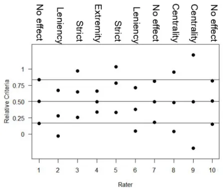
Figure 3.1 is a relative criterion plot for the equal perception model showing the various rater effects generated in the four simulation studies. For the equal perception model, the relative response criterion is calculated as each estimated criterion parameter divided by the estimated distance between the highest and lowest latent perception distributions for each rater,cjk/[(K -1)×dj] (DeCarlo, 2005). Then, it is possible to compare rater effects among each rater. Raters 1, 7, and 10 have no rater effects since their estimated criteria are located on the lines. Raters 8 and 9 have centrality effects since their first criteria are below the optimal line and their third criteria above the line. Since the criteria are thresholds of assigning scores, these two raters will never give scores of 1 or 4. Rater 4 has extremity effect since her first criteria are above the optimal line and her third criteria below the line. Raters 2 and 6 are lenient since their three criteria are all below the lines. Raters 3 and 5 are strict since their three criteria are all above the lines.
Data generation
The data were simulated with modified SAS macros by DeCarlo (2005). 10 raters discriminated between four latent classes and assigned a score of 1-4. The latent class sizes followed an approximately normal distribution, in consistency with the results from analyses of real-world data (DeCarlo, 2008b). The logistic-model values ofdfrom 0.5–5.5 were used, which means moderate to excellent rater precision (DeCarlo, 2008b). Distance less than 0.5 is small, over 2 big, and around 1 medium (DeCarlo, 2002, 2005). Without rater effects, the criteria are located at the interaction of adjacent latent perception distributions. Each condition had a sample
Figure 3.3. Relative Criteria Parameters for a 4-class Equal Perception Model. The plot shows relative response criteria for each rater as filled circles and optimal location points as lines. Names of rater effects are shown on top.
size of 1,000 and 100 datasets. The process of data generation followed three steps as in DeCarlo (2008b):
1. Generate the values for the latent variableη(0, 1, 2 and 3) with a multinomial distribution. The probability for each latent category followed the size of each latent class.
2. Generate cumulative response probabilities for raters and response categories with a logistic distribution forF. Plugηobtained in step 1 together with population
parameterscrkjanddrjinto Equation 5 orcrkjanddrkj into Equation 12.
3. Generate an observed response. The probabilities generated in step 2 were compared to the value of a uniform random variable sampled from 0–1. The response was assigned 1, if the value of the uniform random variable was smaller than or equal to the probability of the lowest response category; was assigned 2, if the value was
greater than the probability of the lowest response category but smaller than or equal to the probability of the second response category; and so on.
Model estimation
Latent Gold 5.1 (Vermunt & Magidson, 2016) was used to fit the equal and ordered perception models. First, simulation studies showed that Version 4.5 had good performance for latent class SDT models (DeCarlo, 2008b). Second, Version 5.1 allows for numerous models and constraints. Third, for latent discrete variables, the algorithm in Latent Gold converges hundreds of times faster than Mplus. Latent Gold starts with the EM algorithm and shifts to the Newton-Raphson algorithm when estimate is in the neighborhood of the ML value (Vermunt & Magidson, 2016). Fourth, Bayes methods can handle missing data and boundary parameters such as large
d's. All models were estimated with the PME method.
Note that label switching (McLachlan & Peel, 2000) is a problem that should be tackled before summarizing the results from estimation. It is arbitrary to assign latent classes as 0, 1, 2, 3 or 3, 2, 1, 0. Since the order of the estimated latent classes is arbitrary, it is possible to have two solutions ofdthat have the same log likelihood values but reversed signs. To address this problem, a (+) was added before each latent class in the equations of Latent Gold. The plus imposes a monotonicity constraint on the probability of each latent category so thatd1≤d2≤d3. 3.2 Empirical Study
Essay scores of 2,350 test taker from a large-scale language test were analyzed to
compare the ordered perception model to the equal perception model. The essays were scored by 27 raters using scores of 1-5, each was rated by two raters, and each rater rated from 61 to 354 essays.
Chapter 4
Results
This chapter shows results for the four simulation studies and the real data analysis. The first five sections discuss results for simulated data both without and with rater effects, both for the fully-crossed design and the BIB design. Also shown is how information criteria are useful in picking the correct models. Section 4.6 discusses results for analyses of real data.
4.1 Simulation 1: Equal Perception Data, Fit Equal Perception Model Without rater effects
Table A1.1 shows parameter recovery ofd’sandc’sover 100 replications of the fully-crossed design without rater effects. The recovery was excellent, with all the percent biases below 3% and all the MSE’s below 0.3. The recovery of the latent class sizes was also excellent, with all the percent biases below 1% and all the MSE’s <0.001.
For the equal perception model, the relative response criterion is calculated as each estimated criterion parameter divided by the estimated distance between the highest and lowest latent perception distributions for each rater,cjk/[(K-1)×dj] (DeCarlo, 2005). Then, it is possible to compare rater effects among each rater.
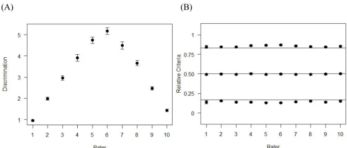
Figure 4.1 shows the distance and relative criteria parameters for the 4-class model. Panel (A) shows a plot of the estimated discrimination parameters with an error bar for each rater which is almost too small to see. The error bar is calculated as
100 2 SD
. It is easy to compare the relative discrimination abilities among each rater and to see that the SE’s of all raters were
negligible. Panel (B) shows relative response criteria for each rater where there were no rater effects as the SE’s of all points overlapped with the lines or optimal locations.
(A) (B)
Figure 4.1. Fully Crossed Design, Distance and Criteria Parameters for a 4-class Equal Perception Model Without Rater Effects, Fit Equal Perception Model. Panel (A) shows
discrimination parameters for each rater and SE bars. Panel (B) shows relative response criteria for each rater and SE bars and optimal location points as lines.
Table B1.1 shows the parameter recovery ofd’sandc’sover 100 replications of the BIB design without rater effects. Compared with its fully-crossed counterpart, the quality of
parameter recovery was a little worse. Although the first criteria ofc's, e.g.,c11, c31, c41, tended to be underestimated by 10%-30%, the biases of other parameters were mostly trivial and all
MSE’s were below 5. For estimates of latent class sizes, the first and fourth classes were overestimated by about 15%, whereas the middle classes were underestimated by slightly over 5%. All MSE’s were around 0.001. Therefore, missing data to some extent degraded parameter estimation.
Figure 4.2 shows the distance and relative criteria parameters. Compared with Figure 4.1, the SE’s were slightly larger, and most SE’s were negligible. Panel (B) shows that there were no rater effects as the SE’s of all points overlapped with or were close to the lines or optimal
locations. Therefore, although missing data increased the percent biases ofd’s andc’s and the SE’s ofd’s, they had little effects on detection of rater effects.
(A) (B)
Figure 4.2. BIB Design, Distance and Criteria Parameters for a 4-class Equal Perception Model Without Rater Effects, Fit Equal Perception Models. Panel (A) shows discrimination parameters for each rater and SE bars. Panel (B) shows relative response criteria for each rater, SE bars, and optimal location points as lines.
With rater effects
Table A1.2 shows the parameter recovery ofd’sandc’sover 100 replications of the fully-crossed design with rater effects. The recovery of parameters was excellent, similar to that of the fully-crossed simulation without rater effects, with all the percent biases below 3%. Note that a dash was used to supersede the infinity percent bias of the estimate ofc21which occurred because of a 0 true value. Dashes were also used for other percent biases of true values of 0. The MSE’s were mostly below 0.5, except for the largestc53which was slightly over 1. The recovery of the latent class sizes was also excellent, as the percent biases were all below 2% and the MSE’s were all <0.001. Similar parameter recovery between without and with rater effects means that adding rater effects in the fully-crossed design had little effect on estimation of model parameters and latent class sizes.
Figure 4.3 shows the distance and relative criteria parameters for the 4-class model. Panel (A) shows that compared with the fully-crossed simulation without rater effects in Figure 4.1, the SE’s were a little larger. Panel (B) shows that all the generated rater effects were perfectly
caught. For example, either Rater 8’s or Rater 9’s obtained first relative criterion was lower than the optimal first relative criterion and both of their obtained third relative criteria were high than the optimal third relative criteria, meaning that those two raters had centrality effects. They were more likely to assign scores 2 and 3.
(A) (B)
Figure 4.3. Fully Crossed Design, Distance and Criteria Parameters for a 4-class Equal Perception Model with Rater Effects, Fit Equal Perception Model. Panel (A) shows
discrimination parameters for each rater and SE bars. Panel (B) shows relative response criteria for each rater and SE bars and optimal location points as lines.
Table B1.2 illustrates the parameter recovery ofd’sandc’sover 100 replications of the BIB design with rater effects. Compared with its fully-crossed design counterpart, the quality of parameter recovery was a little worse. Although the first criteria ofc's, e.g.,c11, c41, c51, tended to be underestimated by 10%-60% and boundaryd's tended to be underestimated by around 20%, the biases of other parameters were mostly trivial. The MSE’s were mostly below 1, except for the largest parameters. For estimates of latent class sizes, the first and fourth classes were
overestimated by about 10%-15%, whereas the middle classes were underestimated by about 5%. The MSE’s were around 0.001. Once again, this comparison shows that missing data somewhat biased the estimation of parameters.
Figure 4.4 shows the distance and relative criteria parameters for the 4-class model of the BIB design with rater effects. Panel (A) shows that compared with Figure 4.2, the SE’s were slightly larger, which means that for BIB design adding rater effects had little effect on SE’s of parameter estimation. Raters 1 and 10 had the smallest standard errors whereas Raters 3-8 had the largest. Raters 5 and 6 had large, negative biases for theird’s, and these two raters had the highest trued’s and relatively large criteria shifts-up 2 ford5and down 2 ford6. So, large rater effects can bias thed’s a little. Panel (B) shows that all rater effects were determined. Once again, it was found that missing data had little effect on detection of rater effects.
(A) (B)
Figure 4.4. BIB Design, Distance and Criteria Parameters for a 4-class Equal Perception Model with Rater Effects, Fit Equal Perception Models. Panel (A) shows discrimination parameters for each rater and SE bars. Panel (B) shows relative response criteria for each rater, SE bars, and optimal location points as lines.