CONCEPTUAL DESIGN AND SAMPLING PROCEDURES OF THE BIOLOGICAL PROGRAMME OF NUUKBASIC

(1)

Scientifi c Report from DCE – Danish Centre for Environment and Energy No. 158 2015

CONCEPTUAL

DESIGN

AND

SAMPLING

PROCEDURES

OF

THE

BIOLOGICAL

PROGRAMME

OF

NUUKBASIC

2nd edition

AARHUS

UNIVERSITY

DCE – DANISH CENTRE FOR ENVIRONMENT AND ENERGY

AU

(2)

(3)

Scientifi c Report from DCE – Danish Centre for Environment and Energy 2015

AARHUS

UNIVERSITY

DCE – DANISH CENTRE FOR ENVIRONMENT AND ENERGY

AU

CONCEPTUAL DESIGN AND SAMPLING PROCEDURES

OF THE BIOLOGICAL PROGRAMME OF NUUKBASIC

2nd edition

Peter Aastrup1 Josephine Nymand2 Katrine Raundrup2 Maia Olsen2 Torben L. Lauridsen1

Paul Henning Krogh1

Niels Martin Schmidt1

Lotte Illeris3

Helge Ro-Poulsen3

1_{Aarhus University, Department of Bioscience} 2_{Greenland Institute of Natural Resources}

3_{University of Copenhagen, Department of biology}

(4)

Data sheet

Series title and no.: Scientific Report from DCE – Danish Centre for Environment and Energy No. 158 Title: Conceptual design and sampling procedures of the biological programme of

NuukBasic

Subtitle: 2nd edition

Authors: Peter Aastrup1, Josephine Nymand2, Katrine Raundrup2, Maia Olsen2, Torben L. Lauridsen1, Paul Henning Krogh1_{, Niels Martin Schmidt}1_{, Lotte Illeris}3_{& Helge}

Ro-Poulsen3

Institutions: 1Aarhus University, Department of Bioscience, 2Greenland Institute of Natural Resources & 3University of Copenhagen, Department of Biology

Publisher: Aarhus University, DCE – Danish Centre for Environment and Energy © URL: http://dce.au.dk/en

Year of publication: August 2015 Editing completed: May 2015

Quality assurance, DCE: Vibeke Vestergaard Nielsen

Financial support: The present project has been funded by the Danish Energy Agency as part of the climate support programme to the Arctic. The authors are solely responsible for all results and conclusions presented in the report, and do not necessary reflect the position of the Danish Energy Agency.

Please cite as: Aastrup, P., Nymand, J., Raundrup, K., Olsen, M., Lauridsen, T.L., Krogh, P.H:, Schmidt, N.M., Illeris, L. & Ro-Poulsen, H. 2015. Conceptual design and sampling procedures of the biological programme of NuukBasic. 2nd edition. Aarhus University, DCE – Danish Centre for Environment and Energy, 68 pp. Scientific Report from DCE – Danish Centre for Environment and Energy No. 158 http://dce2.au.dk/pub/SR158.pdf

Reproduction permitted provided the source is explicitly acknowledged

Abstract: This manual describes procedures for biologic climate effect monitoring in Kobbefjord, Nuuk. The monitoring is a part of NuukBasic which is a cross-disciplinary ecological monitoring programme in low Arctic West Greenland. Biological monitoring comprises the NERO line which is a permanent vegetation transect, and monitoring reproductive phenology of Salix glauca, Loiseleuria procumbens, Eriophorum angustifolium, and

Silene acaulis. The progression in vegetation greenness is followed along the vegetation transect and in the plant phenology plots by measurement of Normalized Difference Vegetation Index (NDVI). The flux of CO2 is measured in natural conditions as

well as in manipulations simulating increased temperature, increased cloud cover, shorter growing season, and longer growing season. The effect of increased UV-B radiation on plant stress is studied by measuring chlorophyll fluorescence in three series of plots. Arthropods are sampled by means of yellow pitfall traps as well as in window traps. Microarthropods are sampled in soil cores and extracted in an extractor by gradually heating up soil. The avifauna is monitored with special emphasis on passerine birds. Only few terrestrial mammals occur in the study area. All observations of mammals are recorded ad-hoc. Monitoring in lakes include ice cover, water chemistry, physical conditions, species composition of plankton, vegetation, bottom organisms and fish. Physical-chemical parameters, phytoplankton and zooplankton are monitored monthly in the ice-free period.

Keywords: Monitoring, arctic, phenology, carbon flux, NDVI, UV-B, arthropods, microarthropods, lake ecology

Layout: Graphic Group, AU Silkeborg Front page photo: Peter Aastrup

ISBN: 978-87-7156-157-9 ISSN (electronic): 2245-0203

Number of pages: 68

(5)

1 Introduction

The Nuuk Basic programme was initiated in 2007 by the National Environ-mental Research Institute, Aarhus University, in cooperation with the Greenland Institute of Natural Resources. BioBasis is funded by the Danish Energy Agency and the Danish Environmental Protection Agency as part of the environmental support programme DANCEA – Danish Cooperation for Environment in the Arctic. The present manual describes methods and sam-pling procedures. The manual will be updated regularly. The latest version can always be found here: www.nuuk-basic-dk

Nuuk Basic is a climate change effects monitoring programme close to Nuuk in west Greenland. The programme studies the effects of climate variability and change on marine and terrestrial ecosystems. In terms of scientific con-cept, Nuuk Basic copies the investigations carried out in Zackenberg Basic, at Zackenberg Research Station in Northeast Greenland

(www.zackenberg.dk).

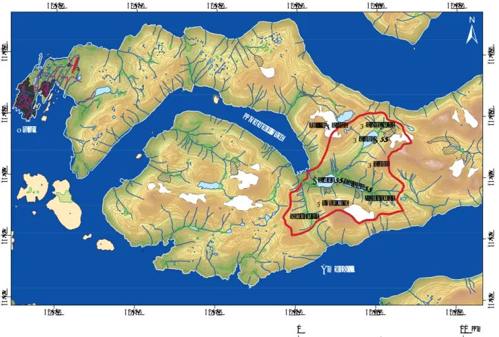
The study area is situated approximately 20 km east of Nuuk as seen on fig-ure 1 and 2. The local climate is low arctic with a mean annual temperatfig-ure of -1.4 °C and a mean annual precipitation of 752 mm (1961-90). The drain-age basin is situated in an alpine landscape with mountains rising up to 1400 meter above sea level and with glacier coverage of approximately 2 km2_.

Geologically, the area is homogenous with Precambrium gneisses as base-ment throughout the drainage basin.

0 10 Km Qassi Langsø Badesø Yderdal Inderdal Qassi Sø Qassi dal Storfjeld Lille-Qassi 51°42'W 51°36'W 51°30'W 51°24'W 51°18'W 51°12'W 51°42'W 51°36'W 51°30'W 51°24'W 51°18'W 51°12'W 64°12'N 64°10'N 64°8'N 64°6'N 64°4'N 64°12'N 64°10'N 64°8'N 64°6'N 64°4'N Nuuk Ameralik Kobbefjord

(8)

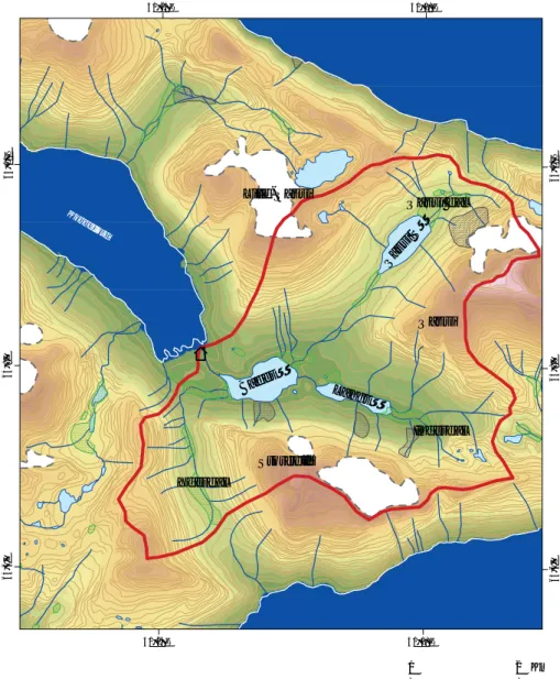
Figure 2. Close-up of the

BioBasis study area.

Qassi Langsø Badesø Yderdal Inderdal Qassi Sø Qassi dal Storfjeld Lille-Qassi Kobbefjord d 51°24'W 51°18'W 51°24'W 51°18'W 64°10'N 64°8'N 64°6'N 64°10'N 64°8'N 64°6'N 0 2 Km

(9)

7

2 Overview of monitoring elements

2.1 Plants

Table 1 gives an overview of the monitoring of plants.

2.1.1 The NERO-line

The NERO line is a permanent vegetation transect which was established in July 2007 in order to monitor future changes in the distribution and compo-sition of vascular plant species in the plant communities (Bay et al. 2008). Surveys of the transect will take place with 5 year intervals. In 2010 mosses and lichens were included in the monitoring programme.

Table 1. Overview of monitoring elements Monitoring element Species Number of plots Sampling frequency Sampling object Sampling period

NERO-line Plant communities and species Every 5th year

Phenology Salix glauca 4 Weekly Buds, flowers, and seeds. May- October Loiseleuria procumbens Buds, flowers, and seeds May- October

Silene acaulis Buds, flowers, and seeds

Vegetation analysis – pin point analysis – to be done

4 per plot Every 5th year Plot – four subplots per plot

-

Total count of flowering shoots

Salix glauca Once per season

at peak flowering Flowers Depending on phenology Loiseleuria procumbens Silene acaulis Eriophorum angustifolium

NDVI Along vegetation transect Monthly May- October

In phenology plots, plots with Eriophorum angustifolium, and plots with Empetrum nigrum

16 weekly May- October

CO2 - Flux Control, C 6 plots per treatment

Weekly Plot May- October

Increased temperature, T Shading, S

Long growing season, LG Short growing season, SG

UVB Control 5 3 plots weekly,

week 29-31 Mylar film (0,25 mm)

Filter control (Teflon)

Arthropods All taxonomic groups 4 plots - 8 subplots weekly specimens May - October

MicroAr-thropods

Collembolan species 8 plots 3 times per season specimens June - Septem-ber Orbatid and actinedid mites

and others

Birds Passerines etc. Mammals Ad hoc

Lakes Water chemistry Two lakes 5 times per season June – October

Flora Every year (ice-free period)

Fauna Every 5th year

Arctic char, Stickleback

(10)

The concept relies on the assumption that changes in the distribution of plant communities can be seen by changes of boundary lines between vege-tation zones. Therefore each boundary between vegevege-tation zones has been marked by a peg. The species composition of the vegetation zones has been documented by Raunkjær analyses. Immigration of new species is assumed to be documented by the surveys with five year intervals. The concept is also used for the ZERO line in Zackenberg in high arctic North East Greenland (Fredskild & Mogensen 1996, Bay 2001, 2006).

Movement of zones is documented by the position of pegs, while changes in species composition are recorded by Raunkjær analyses.

2.1.2 Reproductive phenology

It is expected that plant phenology will give an early and distinct response to climate change. This has already convincingly been shown in Zackenberg. In Nuuk we follow four species: Salix glauca, Loiseleuria procumbens, Eriophorum angustifolium and Silene acaulis. These species were chosen because they are widely distributed in the area, they cover a spectrum of different growth forms (deciduous dwarf shrub, evergreen dwarf shrub, graminoids and cushion forming herb), and they are comparable to species monitored in Zackenberg.

For each species four observation plots were established. The specific sites of the plots were chosen in order to cover the ecological amplitude of the spe-cies with respect to duration of snow cover, difference in soil moisture at the site and altitude. The size of each plot varies depending on the abundance of individual flowering shoots of the species in question.

2.1.3 Total flowering

Total flowering in the reproductive phenology plots is followed for Salix glauca, Loiseleuria procumbens, Eriophorum angustifolium, and Silene acaulis. The number of flowers is counted at peak flowering as the total number of buds, flowers (catkins in Salix) and senescent flowers (catkins in Salix).

2.1.4 Normalized Difference Vegetation Index (NDVI)

The progression in vegetation greenness is followed along the vegetation tran-sect (the NERO line), in the plant phenology plots and in the CO2 flux plots

by measuring NDVI with a scanner. NDVI is used as an index of plant pro-duction and vigorousness. The scanner measures the spectral reflectance of the plant canopy.

2.1.5 CO2 flux plots

The CO2 flux is important for understanding the balance between CO2

emis-sion and uptake. This study aims at documenting the present state, but it will also provide data from manipulations simulating increased temperature and increased cloud cover, shorter growing season, and longer growing season.

2.1.6 UV-B exclusion

UV-B radiation will increase as a result of the expected depletion of the ozone layer in the atmosphere. We monitor the effect of increased UV-B ra-diation on plant stress indirectly by measuring chlorophyll fluorescence in

(11)

9 three series of plots: Controls, plots with a filter excluding UV-B, and filter controls with a film without exclusion of UV-B. Measurements of chloro-phyll fluorescence are carried out in Betula nana and Vaccinium uliginosum in a mesic dwarf shrub heath dominated by Empetrum nigrum and with Betula nana and Vaccinium uliginosum as subdominant species.

2.2 Arthropods

Arthropods are sampled by means of yellow pitfall traps. Window traps are used for flying insects. The traps are emptied weekly throughout the sum-mer season. Samples are stored at Greenland Institute of Natural Resources (GINR) and shipped to Department of Bioscience, Aarhus University, Silke-borg.

2.3 Microarthropods

Soil cores are collected with a soil corer from which the organisms are ex-tracted in a heat extractor by gradually heating up. Microorganisms are de-termined at Department of Bioscience, Aarhus University, Silkeborg.

2.4 Birds

The avifauna is monitored with special emphasis on passerine birds repre-senting the highest trophic level. Breeding phenology (first egg dates, hatch-ing, fledging) is monitored throughout the season on an ad hoc basis.

Weekly counts of birds are carried out at census points during the entire sea-son. Other bird observations are recorded ad-hoc during the entire field seasea-son.

2.5 Mammals

Only few terrestrial mammals occur in the study area and only very sporad-ically: Arctic fox Alopex lagopus, arctic hare Lepus arcticus, and caribou Rangi-fer tarandus. All observations of mammals are recorded ad-hoc. If arctic fox dens are discovered, reproduction will be followed.

2.6 Lakes

The two sampling lakes are located in the Kobbefjord catchment area in the bottom of Kobbefjord (Badesø / Kangerluarsunnguup Tasia: 64,13ºN, 51,36ºW and Qassi Sø: 64,15ºN, 51,31ºW).

Monitoring include ice cover, water chemistry, DOC (dissolved organic car-bon), chlorophyll a, physical conditions, species composition of plankton, vegetation, bottom organisms and fish. Physical-chemical parameters, DOC, chlorophyll a, phytoplankton and zooplankton are monitored monthly in the ice-free period.

(12)

3 Detailed manual

Appendix 1 gives an example of the activities during a monitoring season in Kobbefjord. In the following paragraphs procedures are described in detail for all monitoring elements.

3.1 Plants

3.1.1 The NERO line

The NERO line was established in 2007. It is described in detail in Bay et al. (2008 - http://www2.dmu.dk/Pub/FR693.pdf). Surveys of the vegetation transect are done with 5 year intervals. Next survey of the line is expected in 2017. The location of the line is shown in figure 3. See also Bay et al. 2008).

Figure 3. The NERO line. The

dots show the positions of the pegs and the colour indicate the vegetation zone northeast of the peg. Numbering of the pegs starts in the south-western cor-ner. The break in the long black line to the north-east marks a steep slope that was not ana-lysed by Raunkjær analyses and pin-point analyses. The short line represents the coastal zone. The black square shows the position of the characteristic, but rare plant community dominated by Deschampsia flexuosa and Jun-cus trifidus, which is found on south facing, dry slopes. The map is based on GPS-positions (accuracy 5-10 m). Bedrock Bedrock/heath Copse Fen Heath Lake River River bed Salt marsh Snow-patch Badesø Kobbefjord

Main vegetation transect Salt marsh transect

Deschampsia-Juncus transect

64°8'N

(13)

11

Input of data into database

Data from the Raunkjær circle analyses are entered into an Access data base with the columns Peg no., Plot no., Year, Month, Day, Observer, Vegetation type, species name, Raunkjær value, Uncertain species identifications have cfr. (=confer) added to indicate the need for further confirmation. Fertility is given by Flowering added next to the Raunkjær value.

Digital pictures are kept at the Greenland Institute of Natural Resources backup server.

3.1.2 Reproductive phenology

The monitoring consists of weekly counts of buds, flowers, and senescent flowers to monitor the proportion of buds, flowers and senescent flowers of the species: Salix glauca, Loiseleuria procumbens, and Silene acaulis.

Species to be monitored

Three species: Northern willow Salix glauca, Trailing azalea Loiseleuria pro-cumbens, and Moss campion Silene acaulis

• Are commonly found in the area.

• Cover a spectrum of different growth forms (deciduous dwarf shrub, ev-ergreen dwarf shrub, and cushion forming herb/dwarf shrub.

• Are comparable to species monitored by BioBasis in Zackenberg.

There are four plots for each species. The size of each plot varies (see table 2) depending on the abundance of individual flowering shoots of the species in question.

Frequency of sampling

Censuses of Salix glauca, Loiseleuria procumbens, and Silene acaulis are made at weekly intervals in the snow free season (normally May – October). Total counts of flowers are done once a year at peak flowering.

Equipment

• Map with position of study plots (+GPS)

• Data form Appendix 2/ Notebook. Location and marking of study plots

The positions of the 12 study plots are shown in Figure 4. The plots are marked with angle pegs in each corner. The plots are divided into four sec-tions (quarters A, B, C, and D separated by pegs at the centre where the di-agonals cross and at the midpoint of each side – see Figure 5). The lettering starts at the corner with the plot-ID and continues clockwise around the cen-tre. Co-ordinates, dimensions etc. appear from table 2.

(14)

Figure 4. The locations of the

plant reproductive phenology plots and plots for annual total counts of flowering shoots for Salix glauca (SAL1-SAL4), Silene acaulis (SIL1-SIL4), and

Loiseleuria procumbens (LOI1-LOI4). Note that for Eriophorum angustifolium (ERI1-ERI4) only total counts of shoots are carried out. Coordinates can be found in table 2. LOI4 LOI3 LOI2 LOI1 SIL3 SIL2 SIL1 SIL4 SAL4 SAL3 SAL2 SAL1 _ERI4 ERI3 ERI2 ERI1 Badesø Kobbefjord 64°8'N 64°8'N 0 0.5 Km

Table 2. Positions and sizes of plant reproductive phenology plots. Positions are given in

decimal degrees.

Species Plot Latitude Longitude Plot dimensions (m)

Eriophorum nigrum ERI1 64,1346 -51,3837 4*10 ERI2 64,1312 -51,3873 10*10 ERI3 64,1348 -51,3789 6*8,5 ERI4 64,1333 -51,3666 5*9

Salix glauca SAL1 64,1325 -51,3729 7*11

SAL2 64,1316 -51,3714 8*8

SAL3 64,1337 -51,3678 6*9

SAL4 64,1374 -51,3741 4*5

Silene acaulis SIL4 64,1361 -51,3681 5*12

SIL1 64,1328 -51,3745 5,5*7 SIL2 64,1364 -51,3703 11*11 SIL3 6,4137 -51,3736 7*11 Loiseleuria procumbens LOI1 64,1323 -51,3759 1,8*3,85 LOI2 64,1316 -51,3705 1,7*2,95 LOI3 64,1324 -51,3708 1,6*2,6 LOI4 64,1328 -51,3702 1,6*3,0

(15)

13

Sampling method

The following observations and censuses are entered into the relevant data forms for all plots:

• Time

• Cloud cover

• Plot number

• Snow cover

• Number of buds

• Number of flowers (catkins in Salix) – note that for Salix both male and female plants can be found in the plots

• Number of senescent female catkins with hairs (Salix)

• Number of senescent flowers (Loiseleuria and Silene)

• Total number of flowers (Salix, Eriophorum, Silene and Loiseleuria)

• Occurrence of larvae, fungi etc.

Data forms are found in Appendix 2. The data from the weekly counts of the plots are entered into data files with columns relevant for each species. The basic data are: Year, Month, Day, Photo no., Observer, Species (SAL, LOI, SIL, ERI), Plot (1-4), Subplot (A-D), Snow (percent in sector), Cloud cover (x/8), Buds (actual numbers counted, not percent), Flowers, Senescent (flowers), Total (sum of buds, flowers and senescent flowers), Larvae, Fungi and Remarks. Specific columns for individual species appear from the data-base files.

During snow melt in May/June, percent snow cover in each plot section is estimated at each sampling trip. If any plant part is visible above the snow layer, the cover is given as 99%. If any ground/vegetation cover is free, no more than 98% can be stated.

When visiting Silene plots, samples of a total of 50 flower buds, flowers or senescent flowers (or capsules with exposed seeds) are recorded within each subplot. In the Salix and Loiseleuria plots a total of 100 buds, flowers and se-nescent flowers are recorded. This is done by counting the different

pheno-Figure 5. Lettering of subplots in

plant phenology plots. The dot indicates the corner with the plot ID. Arrows indicate clock-wise round direction for

NDVI-measurements.

B

C

(16)

logical stages until a total of 50/100 is achieved. Begin to the right in each section and count towards the left. Avoid biasing the count by actively se-lecting a starting point other than the right corner.

In general, flower buds are defined as flowers not yet open, flowers are open giving insects access to the reproductive organs, and senescent flowers as flowers that have lost all petals or with all petals almost or fully faded or brown. In some of the final stages, flower stems from the preceding year may interfere with the counts. However, such old stems are always dry and stiff; stems of this year are soft and fleshy.

For each species, the following sampling procedures apply in particular. Salix

The sampling unit is catkins, not individual flowers. Most flowers from one catkin emerge the same day, and they also wilt at the same time. Hence, cat-kins are recorded as buds (Figure 6), when no stigmas or anthers are visible, and as male (Figure 7) and female (Figure 8) flowers as soon as anthers (m) or stigmas (f) are visible (they are often both red in the early stages, but the colour may vary).

Both senescent flowers and fruits continue to be recorded as 'flowers' until they are recorded as having exposed seed hairs (Figure 9) from the time of exposure of the first hairs on top of the splitting capsules. Notice that fruits may be affected by larvae so that they expose seed hairs from the bottom of the capsules (excreta from the larvae are often visible among the seed hairs). These capsules must not be recorded as having seed hairs exposed, but should be recorded separately. In Kobbefjord this has not been seen yet.

Fruits infected by sponges (yellow and twisted) should be recorded separately (yet still included in the number for 'flowers', i.e. the infected fruits appear twice in the data forms). Also, infections by insects should be recorded.

Figure 6. Salix glauca buds. It is

not possible to discriminate be-tween male and female flowers at this stage.

(17)

15

Figure 7. Salix glauca male

flowers.

Figure 8. Salix glauca female

(18)

Silene

Silene acaulis grows in hummocks (Figure 10) and one or a few specimens may dominate the sample.

Flower buds are reddish or light purple (Figure 11). Senescent flowers (Fig-ure 12) have wilted petals or appear as empty “cups” (Fig(Fig-ure 12). Senescent flowers are defined as flowers with faded petals and empty pollen anthers.

Figure 9. Senescent Salix glauca

(19)

17

Figure 10. Silene acaulis

hum-mock.

Figure 11. Silene acaulis –

flow-ers in the foreground. The buds in the background should be recorded as buds even though they are close to opening as flowers.

(20)

Loiseleuria

Loiseleuria procumbens is a matted shrub with pairs of tiny, oblong, closely-set leaves and abundant clusters of small flowers, see Figure 13. In Greenland plants are not taller than 10 cm. The plant is creeping, much-branched, mat-forming, with 2-5 pink, bell-shaped flowers in terminal clusters and ever-green leaves with rolled edges.

The data from the weekly registrations are entered into Excel data sheets with columns relevant for each of the three species. Year, Month, Day, Photo no., Observer, Species (SAL, LOI, SIL, ERI), Plot (1-4), Subplot (A-D), Snow (percent in sector), Cloud cover (x/8), Buds (actual numbers counted, not

Figure 12. Silene acaulis –

se-nescent flowers – in the middle still with wilted petals.

Figure 13. Loiseleuria

procum-bens. Half open flowers, opening buds, closed buds and senescent flowers from last year.

(21)

19 percent), Flowers, Senescent (flowers), Total (sum of buds, flowers and se-nescent flowers), Larvae, Fungi and Remarks. Specific columns for individu-al species appear from the data base.

3.1.3 Total flowering

Northern willow Salix glauca, Trailing azalea Loiseleuria procumbens, Moss campion Silene acaulis, and Cotton grass Eriopherum angustifolium. See previ-ous section for descriptions of Salix glauca, Loiseleuria procumbens, and Silene acaulis. E. angustifolium is described below.

Eriophorum

Eriophorum angustifolium flowers are monoecious (individual flowers are ei-ther male or female, but both sexes can be found on the same plant) and are pollinated by wind. There are two or more flowers on each stem. There are two or more fruiting heads per plant, which distinguishes it from the other common species, Arctic cotton grass. Figure 14-15 shows different stages of Eriophorum flower development.

Figure 14. Eriophorum

(22)

Once per season. Total counts of S. glauca, L. procumbens, and S. acaulis are made at peak flowering. The optimal time for total counts of E. angustifolium is when most or all flower buds have reached senescence.

• Equipment

• Map with position of study plots

• Pieces of cord totalling 100 m

• Flower sticks

• Tally counters

• Data form Appendix 2/ Notebook. Location and marking of sampling plots

The plots are divided into four subplots (A, B, C, and D) separated by steel pegs at the centre where the diagonals cross and at the midpoint of each side. The lettering starts at the corner with the plot-ID and continues clock-wise around the centre. Co-ordinates, dimensions etc. appear from table 2.

Figure 15. Eriophorum

(23)

21 The plots are identical with the plant reproductive phenology plots shown in figure 4.

Sampling method

Tighten a cord around each section of the plot. In large plots, subsections are established by placing two additional cords with about 0,5 or 1 m intervals from one end of each section, whereupon the summed number of flower buds, flowers, and senescent flowers, respectively, are counted between each cord. Move one cord at a time and repeat the process until the entire plot is covered. In small plots, sticks may be used instead of cords. In the Salix plots, male and female catkins are counted separately. Catkins that have been grazed, but can still be sexed, are included.

The data from the yearly registrations are entered into Excel data sheets with columns relevant for each of the three species. Year, Month, Day, Photo no., Observer, Species (SAL, LOI, SIL, ERI), Plot (1-4), Subplot (A-D), Snow (cent in sector), Cloud cover (x/8), Buds (actual numbers counted, not per-cent), Flowers, Senescent (flowers), Total (sum of buds, flowers and senes-cent flowers), Larvae, Fungi and Remarks. Specific columns for individual species appear from the data base.

3.1.4 Normalised Difference Vegetation Index (NDVI) in plots and along the NERO line

The progression in the vegetation greenness is followed along the vegetation transect (the NERO line) and in the plant phenology plots. The monitor measures the spectral reflectance of the plant canopy.

Species or taxonomic groups to be monitored

All vegetation types along the NERO line between VT001 and VT076.

All plants in the reproductive plant phenology plots. Frequency of sampling

Along the NERO line: Monthly.

Plant phenology plots: Weekly in connection with the plant phenology cen-suses.

Equipment

• Map of vegetation transect and plant phenology plot positions

• GPS with positions of vegetation transect and phenology plot positions

• Crop Circle Handheld system. A handheld Crop Circle TM ACS-210 Plant Canopy Reflectance Sensor which calculates the greening index (NDVI).

• Notebook

• Digital camera.

Location and marking of sampling plots

The NERO line crosses all the dominating vegetation types found in the study area. The NERO line is described in detail in Bay et al. 2008. The measurement is carried out 5 m north-east of the vegetation transect. Sur-veying rods mark the transect to be scanned.

(24)

Plant phenology plots: See Table 2 and Figure 4. Sampling method

NDVI is measured by The Crop Circle Handheld System which integrates a Crop Circle ACS-210, GeoSCOUT GLS-400 and a FieldPAK PS-12 into a single instrument (See Figure 16). Data is collected and stored on a SD flash disk.

The procedure is:

1. Insert an empty SD flash card into the card slot

2. Turn on the CropCircle system by pressing the ON/OFF button 3. Press the DISP button to select MAP mode. Then press OK

4. When ready press LOG and the CropCircle starts to measure NDVI 5. Use the trigger switch also connected to the CropCircle between each

subplot (A, B, C, and D)

6. Turn the CropCircle OFF after each plot in order for the data to be saved on the SD flash card.

Scans are conducted by moving the sensor steadily forward (ca. 1 meter per second) approximately 75 cm above the vegetation. This results in a measur-ing footprint of approximately 10 x 45 cm. Refer to the CropCircle manual for more information.

The following sampling order must be applied (table 3). Also, always meas-ure all plots in the order A-D (see Figmeas-ure 5). At each visit, note under Re-marks the presence of snow (snow in subplot; snow at plot edge) and if the vegetation is moist.

Figure 16. Equipment for

meas-uring NDVI – the Crop Circle Handheld System.

(25)

23 All measurements are conducted only on the AB and the CD sides of the plots (Figure 5). Place yourself at the plot number plate, just outside the plot. Hold the sensor approximately 50 cm into the subplot at the subplot edge. Switch on the NDVI logger (switch on the left of the stage), and walk slowly (approximately 1 m per second) along the sides indicated by arrows on fig-ure 5. Use the trigger switch to pause the NDVI logger at the next corner of the subsection. Repeat the procedure in the remaining subsections. Hence, four scans are made in each of the vegetation plots. Turn off the Crop Circle system between plots by pressing the ON/OFF button.

When measuring the NERO line always start at the top of the slope and walk towards the river.

Ideally all plots and transects on both sides of the river should be measured on the same day. If the vegetation is wet, the measurements must be post-poned to the following day.

Data is downloaded from the SD card from the CropCircle using a card reader. The CropCircle automatically names the files (e.g. ddmmyyAA.CSV; ddmmyyAB.CSV; etc.) Each file holds the following variables: Longitude, Latitude, Elevation, Fix Type, UTM Time, Speed, Course, SF1, SF2, SF3, SF4, SF5, and SF6. All Crop Circle data files are saved separately. In Excel, each data file is supplemented with the following columns: Year, Month, Day, DOY, Observer, Plot, Subplot, and Remarks. All files are merged into one sheet in one file. Please notice that if your computer is set with a Danish Of-fice-version the ddmmyyAA-file may be the last file in the file list since the AA is regarded as Å (but it is still the first one recorded).

Digital pictures are stored at the Greenland Institute of Natural Resources backup server (F:\40-59 PaFu\41 Vegetation\08 NuukBasic_BioBasis). Pic-tures are named PlotPlotno_Date (e.g. SAL1_110930).

Table 3. Sequence of phenology plots and NDVI.

ERI1 (Eriophorum 1) EMP1 (Empetrum 1) ERI2 (Eriophorum 2) EMP2 (Empetrum 2) ERI3 (Eriophorum 3) EMP3 (Empetrum 3) LOI1 (Loiseleuria 1) SIL1 (Silene 1) SAL1 (Salix 1) SAL2 (Salix 2) LOI2 (Loiseleuria 2) LOI3 (Loiseleuria 3) LOI4 (Loiseleuria 4) ERI4 (Eriophorum 4) EMP4 (Empetrum 4) SAL3 (Salix 3) SIL4 (Silene 4) SIL2 (Silene 2) SIL3 (Silene 3) SAL4 (Salix 4)

(26)

3.1.5 Normalised Difference Vegetation Index (NDVI) in CO2 flux plots

The progression in the vegetation greenness is followed in the CO2 flux

plots. The monitor measures the spectral reflectance of the plant canopy as well as the incoming light using two sensors.

Species or taxonomic groups to be monitored All plants in the CO2 flux plots.

Weekly in connection with the CO2 flux measurements.

Equipment

• Map of CO2 flux plot positions

• GPS with positions of CO2 flux plot

• A handheld SpectroSense 2+ system including two light sensors (marked 38291 and 38294 respectively) which calculates the greening index (NDVI). See figure 17

• Data form Appendix 3A or 3B / Notebook. Location and marking of sampling plots CO2 flux plots: See figure 20.

Sampling method

NDVI in the CO2 flux plots is measured by the SpectroSense 2+ system

which integrates the analysing apparatus / the device with two light sen-sors. Data is not stored, and must be written in the “Remarks” section on ei-ther data form 3A or 3B.

The procedure is:

1. Fasten the 4 metal legs/rods loosely to the Plexiglas plate using the ac-companying screws and bolts. The legs should be fixed but able to turn slightly to fit into the metal frame in the plots – one leg in each corner. This ensures identical measurement height every time.

2. Unscrew the bolt on the light sensors and attach the sensors to the Plexi-glas plate as follows: attach the sensor marked 38291 with a diffuser in the hole outside the “square” made out of the 4 bolts from the legs. The 38291 sensor must face upwards. Attach the sensor marked 38294 with-out a diffuser in the hole in the middle of the “square” between the bolts from the legs. The 39284 sensor must face downwards.

3. Connect the light sensor marked 38291 with a diffuser in the “Current C1/C3” (plug no. 2 from the left) on the device. See figure 17.

4. Connect the light sensor marked 38294 without a diffuser in the “Current C2/C4” (plug no. 3 from the left) on the device. See figure 17.

5. Place the 4 legs connected by the Plexiglas plate with the sensors (double check that the sensors are correctly placed) in the metal frame in the plot. See figure 18.

6. Turn on SpectroSense 2+ with the ON button.

7. Tap the MENU button and scroll down to MENU “6-NDVI” using the ar-row keys on the right hand side. Press ENTER.

8. Initially the NDVI value fluctuates but should reach a fairly stable value after a few seconds. Write the value (with 3 decimals) in the data form 3A or 3B in the remarks column.

(27)

25 9. Continue to the next plot. Do not dismantle the setup between plots. The SpectroSense 2+ may turn off automatically at some point. In that case start at # 7.

10.When all plots have been measured dismantle the legs, Plexiglas plate and unscrew the light sensors but leave the sensor cables in the device until next week.

The easiest way of sampling the plots is by following the same route as when measuring CO2 flux. It may be favourable to do the NDVI measuring

when the flux measurements are completed. Input of data into database

Data is stored in a Excel file with the following columns: Year, Month, Day, Day of Year (DOY), Plot, Treatment, Snow, NDVI and Remarks.

Figure 17. The SpectroSense 2+

device for measuring NDVI in the CO2 flux plots. Attach the light sensors as indicated in the figure.

Figure 18. The light sensors

attached to a plexiglas plate with 4 legs positioned in each of the corners of the flux plot metal frame. Notice the light sensor with the diffuser marked 38291 is facing upwards while the sensor without a diffuser (marked 38294) is facing downwards.

(28)

3.1.6 CO2 flux plots

The ratio between the release of CO2 for photosynthesis and decomposition

of organic matter in the soil, and respiration is measured. The ratio is called Net Ecosystem Exchange (NEE).

The vegetation in the CO2 flux plots which is dominated by Empetrum heath

with Salix as subdominant species. The reproductive phenology of Salix is followed in all plots. Soil moisture is measured in all plots. Temperature is recorded by wireless GeoPrecision mini data loggers.

Carbon fluxes are measured weekly. All plots should be measured between 10 AM and 3 PM, and on the same day.

Equipment

• ITEX-chambers incl. bolts and guy ropes

• Wireless GeoPrecision mini data loggers

• EGM4 – see Figure 21

• Plexiglass measuring chamber (PMC) – measuring 33x33x34 cm (LxWxH).

• Theta-probe for soil moisture measurements

• Black plastic bag adjusted for the PMC

• Sticky Tack

• External 12V battery

• Ruler

• Digital camera

• Data forms Appendix 3A-B/ Notebook. Location and marking of sampling plots

30 plots are situated in a mesic dwarf shrub heath dominated by Empetrum nigrum and with Salix glauca as subdominant species. The heath is facing west. Figure 19 gives an overview of the site and Figure 20 shows the relative posi-tions of the plots.

(29)

27 The setup consists of 5 treatments each replicated 6 times: Control (C), in-creased temperature (T, ITEX hexagons), Shading (S, hessian tents), long growing season (LG, removal of snow during spring) and short growing season (SG, addition of snow during spring).

Temperature is enhanced at T plots by placing hexagonal open top ITEX chambers (OTCs), see Figure 22. This way temperature is expected to in-crease 1-2 ºC during the growing season (for further information, see Molau & Mølgaard, 1996). The shading treatment (S) implies erecting dome shaped sack cloth tents over the soil and vegetation causing an expected 60% reduc-tion of incoming light (Havström et al., 1993).

Figure 19. Overview of CO2 flux plot site with Hessian tents for shadowing and ITEX hexagons for increasing temperature.

Figure 20. Detailed map showing

the position of the CO2 flux plots. The position of the midpoint is 64,14˚N/51,38˚W. For explana-tion of the abbreviaexplana-tions please see text. 1S 1C 1T 1SG 1LG 2SG 2C 2T 2S 2LG 3SG 3C 3T _3S 3LG 4SG 4C 4T 4S 4LG 5SG 5C 5T 5S 5LG 6SG 6C 6T 6S 6LG North

(30)

Short and long growing season plots were supposed to be implemented by respectively adding to and removing snow from SG and LG plots during snow melt at the spring causing plants and soils to be exposed earlier (LG) or later (SG) than in control plots. This has not been done. Instead these plots have been used as controls.

In each of the 30 plots a metal frame of 35x35 cm has been inserted perma-nently into the soil. The frame is used for weekly measurements of ingoing and outgoing fluxes of CO2 to the system by the closed chamber technique.

The metal frames were placed at spots were E. nigrum and S. glauca domi-nated the vegetation. The metal frame is not to be removed by the end of the season.

Sampling method

The CO2 flux plots are established as soon as possible early in the season

(make note of the date). By the beginning of the season, check that the metal frames are level and adjust if needed. Do not adjust the metal frames later or in connection with the gas flux measurements!

The six plexiglas sides of each ITEX hexagon is bolted together in the field, and additionally secured with six guy ropes. Place a wireless GeoPreci-sion mini data logger approximately 2 cm horizontally into the soil. Also place the wireless GeoPrecision mini data logger inside the plot. The wire-less GeoPrecision mini data loggers are programmed to log the temperature every 30 minutes.

Before each measuring round, the EGM must be calibrated to the CO2 level

in the air (the level varies between approximately 365 and 380 ppm). Also, in the lab replace the old Soda lime in the EGM with fresh Soda lime. See the EGM manual for further details (PP Systems 2003). This is done only once a year before the beginning of the season.

Before beginning the gas flux measurements in a plot take a digital ortho-photo covering the entire area inside the metal frame, take three soil mois-ture measurements outside the metal frame but inside the plot using the ThetaProbe. See the ThetaProbe manual for further details, and measure the height (cm) of the upper edge above the ground of the metal frame on the four sides of the frame. Measurements of the chamber height is only done three times during the season (beginning, mid and end of season) in order to avoid unnecessary tear on the vegetation.

Measurement of carbon flux

1. While at the laboratory or in the field cabin make sure the EGM4 is set to take measurements manually (Figure 21). This is done by turning on the EGM4 and press the 2SET button followed by the 5RECD button. The re-cording mode should read 1REC:M. If not press 1REC to get the desired mode. Furthermore check that the handheld computer (YUMA) is set to take automatic measurements every 10 seconds. This is done by starting up the PP Systems Transfer Software, and pressing the “File” bar. Go to “Preferences” and make sure the “Record/Block Interval” is set at 10. 2. In the field place the HTR-2 probe into the plexiglas measuring chamber

(PMC), connect the probe and the tubes from the probe to the EGM4 (in = black tube) and back from the EGM4 to the PMC (out = clear tube). Seal the entrance to the chamber with sticky tack (Figure 21 and 22).

(31)

29 4. Turn on the EGM4 and press 1REC for record by pushing button 1. The EGM4 will have to heat up to approximately 50°C (it may take a while depending on the surrounding temperature). Following the “heating-up” it automatically runs a calibration with the CO2 in the air.

5. Start the PP Systems Transfer Software programme. Press the “Logging” bar and choose the “Auto logging” bar. Select your designated folder and name your file. Press “Save” and then “Pause” immediately afterwards. 6. When the EGM4 has run the calibration (called “Counting Zero”) place

the PMC in the metal frame in the first plot to be measured. Make sure the PMC handle does not cast a shadow on the HTR-2 probe with the PAR measuring device. While measuring gas flux the EGM4 automatical-ly measures the PAR (photosynthetic active radiation) and the tempera-ture in the PMC. The EGM4 may run a calibration while measurements are being taken. The procedure will then have to be repeated from the beginning.

7. The PP Systems Transfer Software is set to automatically take a meas-urement every 10 seconds. Take 13 measmeas-urements under light conditions. Start the first measurement by pressing “Resume” on the YUMA. After the 13th_{measurement press “Pause” on the YUMA. Lift the PMC off the}

frame. Aerate the PMC making sure the CO2 level returns to that prior to

measuring. Monitor the CO2 concentration on the EGM4 or the YUMA.

Place the PMC on the frame again and cover it completely with the black plastic bag. Press “Resume” on the YUMA. After yet another 13 meas-urements press “STOP” on the YUMA. Lift the PMC and aerate it while walking to the next plot to be measured.

8. When all plots have been measured turn off the EGM4.

Measurement of soil moisture

Take three measurements in each plot by pressing the sensor into the soil, read out the soil moisture, and enter data into the form Appendix 3A.

Reproductive phenology of Salix

Reproductive phenology of Salix glauca is followed in all plots according to the procedure described in section 3.1. Data is entered into the form Appendix 3B. Laboratory work

None.

Input of data into the database

Data is saved directly on the handheld computer (YUMA). The raw files are saved in a separate folder (named by the date of measurement) and renamed to include the type of measurements (e.g. 1c, 1t and 1s.dat). In Excel, data are supplemented with the following columns: Year, Month, Day, DOY, Hour, Min, Plot, Treatment, Light, Photo_no, Recno, Cloud cover, Observer, Soil moisture, NDVI (more info in the paragraph on measuring NDVI in CO2

flux plots), Chamber height, and Remarks. All files are merged into one, covering the whole season.

Download digital pictures and rename them to include plot name and date (e.g. ITEX_1C_090602). Save under “Photos” in the folder named “C-flux”.

Data from the wireless GeoPrecision mini data logger is downloaded once a year at the end of the season. Rename the individual files to include plot name and year (e.g. ITEX_5C_2008), and save in a separate folder named “EGM/Temperature”.

(32)

Figure 21. Upper figure shows

the EGM4 which is used for measuring CO2 concentrations. The lower figure shows the top of the instrument.

Figure 22. Measurement of CO2 flux in an ITEX-hexagon open-top chamber with a measuring chamber (PMC) fitted with a HTR-2 probe connected to the EGM4. The black plastic bag is used for dark (respiration) meas-urements.

(33)

31

3.1.7 UV-B exclusion

The impact of ambient UV-B radiation on the vegetation is studied in a me-sic dwarf shrub heath by placing filters approximately 10 cm above the vegetation. At the time of peak plant growth the chlorophyll a fluorescence is measured as an indicator of plant health.

A mesic dwarf shrub heath (facing WSW) dominated by Empetrum nigrum and with Betula nana and Vaccinium uliginosum as subdominant species. The effect of UV-B is measured on Betula nana and Vaccinium uliginosum.

Measurements of chlorophyll fluorescence of leaves of Betula nana and Vac-cinium uliginosum is carried out three times with one week interval at the peak of plant growth (week 29 to 31).

Equipment

• HandyPea fluorimeter (PEA=Photosynthesis Efficiency Analyzer) – See figure 23 and further description below.

• 80 leaf clips

• Data form Appendix 4 / Notebook

• Digital camera

• 5 Frames with UV-B filter (Mylar film, 0.25 mm - with exclusion of UV-B)

• 5 Frames of filter control (Teflon film - without exclusion of UV-B). By the end of the field season, all equipment at UV plots are taken down and brought back to GNIR.

The Handy PEA chlorophyll fluorimeter consists of a control unit. The chlo-rophyll fluorescence signal received by the sensor head during recording is digitised within the Handy PEA control unit. Up to 1000 recordings of be-tween 0.1 - 300 seconds may be saved in the memory of Handy PEA chloro-phyll fluorimeter. Saved data can be viewed onscreen but shall be trans-ferred to a computer for storage and further analysis.

(34)

The sensor unit consists of an array of 3 ultra-bright red LED’s optically fil-tered to a peak wavelength of 650 nm, which is readily absorbed by the chlo-roplasts of the leaf. The LED's are focused via lenses onto the leaf surface to provide even illumination over the area of leaf exposed by the leaf clip (4 mm diameter).

Location and marking of sampling plots

The UVB plots are situated west of the CO2 plots. Figure 24 and 25 gives

overviews of the plots.

There are three series of plots with five replicates:

1. Control - no treatment: C1-C5

2. UV-B filter (Mylar film, with exclusion of UV-B): B1-B5 3. Filter control (Teflon film, without exclusion of UV-B): F1-F5.

Each treatment plot measures 60 cm x 60 cm; the plots are marked with alu-minum tubes at each corner and covered with a frame with the appropriate filter placed approximately 10 cm above the vegetation. During summer the vegetation may grow as tall as the filter, which may then be lifted within the aluminium tubes.

Figure 24. Overview of UV-B

plots.

Figure 25. Schematic

presenta-tion of the locapresenta-tion of UV-B plots. B1

F3 C3 B3 C2 B2 F2 F1 C1 _F4 C5 F5 B5 C4 B4 North

(35)

33

Sampling method

Before establishing the UV plots, filters on frames are checked carefully, and changed if necessary. There is two filter types, Teflon (filter control; the thinnest and most flexible film) and Mylar (excludes UVB; thicker and less flexible). Frame positions are given by small sticks within each plot. UV plots are checked regularly during the entire field season, and repaired if necessary. Specifically, filters in the UV plots must be checked after heavy rain or wind.

The procedure is:

1. Select five green, “healthy-looking” leaves or shoot-tips of Betula nana and Vaccinium uliginosum in each plot.

2. Mount leaf clips on all leaves – preferably without removing the leaf from the branch. Mount on one species at a time. Make sure that the leaf is visible through the hole in the clip and push the shutter to cover the hole so the leaf material is in complete darkness.

3. Keep the shutters closed for at least 30 minutes. The closure time may be longer.

4. Switch on the Handy PEA, Open “main menu” and turn the arrow on the screen to “Measure”.

5. Fit the sensor head to the clip; uncover the hole by pushing the shutter back. Start measuring by pushing “OK” or push the black button on the sensor head. During the measurement a number of parameters appear on the screen. Note that the “Fv/Fb” should be about 0.8. If something goes wrong step three must be repeated before you carry out a new measure-ment.

6. Accept to store the measurement. Note which measurement number cor-responds to each plot.

7. Repeat the sampling now measuring on Vaccinium uliginosum leaves. 8. Take a photo of each plot at each measurement round.

When all measurements have been completed, data must be transferred to a computer by use of the Handy PEA programme. Make sure that all data have been transferred to the computer before clearing the memory in the Handy PEA.

Data are downloaded from the HandyPEA using the PEA Plus software, and the raw files are saved in a separate folder named to include the date of the measurements (e.g. yymmdd.pcs). In Excel, data are supplemented with the following columns: Year, Month, Day, Observer, Species, Treatment, and File no.

3.2 Arthropods

Surface living arthropods are captured in yellow pitfall traps. Flying arthro-pods are captured in wind traps.

(36)

The traps are emptied weekly. If bad weather prohibits visits to the fjord or proper handling of the samples, the traps may be emptied on the earliest day of convenience.

Equipment For field work:

• GPS

• 32 yellow (Pantone no. 108U) plastic cups, 10 cm in diameter and 8 cm deep. Cups have been placed permanently for the season. At the begin-ning of the season it is checked if all cups are placed properly

• Extra yellow cups for emptying the permanent cups

• 4 window traps which are placed permanently

• A thermos

• A garden trowel with sharp edge

• 5 L container for water

• 5 L container for wastewater

• Detergent: Odour free detergent (Coop Änglemark Bluecare Dish washing fluid, concentrated, without perfume, colour and preservation agent)

• Salt (NaCl) without iodine and anti-caking agent

• 20 Metal pegs (to be used in the fen area)

• 1 lady’s stocking per emptying bout

• A pair of flat tweezers

• 36 plastic containers with lids

• 2 L of 70% ethanol

• Small bottle with tip (for rinsing the stocking with alcohol)

• Waterproof speed marker

• Disposable syringes for removal of surplus water

• Ethanol resistant labels

• Pencil

• Water-proof paper

• Ethanol resistant speed marker

• Data form Appendix 5/note book. Location and marking of sampling plots

The position of the study plots are shown on Figure 26. Each plot measures 10 x 20 m and is made up of eight 5 x 5 m squares marked with metal pegs in each corner. Each plot is identified with a number plate, and subplots (with one trap each) are lettered A-H clockwise from the number plate, see figure 27. Sampling method

A set of eight pitfall traps are established in each plot. Each trap is composed of two plastic cups fitting into each other, so that the upper one can be lifted and emptied without disturbing the surrounding soil. The traps are posi-tioned randomly within squares, each of 5 x 5 m, by using the table with random numbers (see the Microarthropod section). The trap is then buried on the nearest reasonably level and ‘elevated’ site (so that it is not flooded during the snow melt) and carefully sunk into the soil, so that the upper rim levels exactly with the soil surface. Place the turf and the removed soil about a meter away from the trap. Do not disperse it, since it must be repositioned after the season, when the traps are removed.

(37)

35 The new traps are placed upside-down during the winter. At the start of the season (i.e. on the round when the traps have appeared from the snow), new clean (washed with a little biodegradable, non-perfumed detergent) upper cups replace the ‘wintering’ ones.

If there is any risk that cups will float up due to water in the lower cup, two metal pegs must be placed along each cup to keep them in position.

The upper cup of the trap is then filled 2/3-3/4 with water (1 l needed per station) added three drops of detergent and a spoonful of salt as killing agent, preservation and to prevent freezing. Use two spoonfuls of detergent and 5 drops of detergent for the wind traps.

Figure 26. Location of arthropod

plots. Art1: Empetrum nigrum heath, Art2: Fen, Art3: Betula nana / Salix glauca heath, Art4: Abrasion. Wind traps are located at Art2 and Art3.

Art4 Art3 Art2 Art1 64°8'N 64°8'N 51°24'W 51°24'W Badesø Kobbefjord 0 0.5 Km

(38)

Emptying the traps

Catches from each of the pitfall traps and wind traps are kept separate. Be-fore emptying a pitfall place the ladies stocking on a spare cup. Then pour the trap liquid through the stocking into the spare cup. Check the trap cup for remaining arthropods and flush with ethanol down into a 100 ml con-tainer should any still remain in the trap. Mites, especially, often remain in the cups. Reposition the pitfall in the soil. The catch from the ladies stocking is now emptied into the 100 ml container by turning the stocking upside down on top of the container. Rinse the inverted stocking with ethanol from the tip of the small bottle. All remaining invertebrates must be removed carefully from the stocking using tweezers and put into the container.

Wind traps are emptied using a plastic spoon with a mesh net. Before emp-tying a wind trap a spare cup is filled (ca. 50%) with water from the trap. Use the spoon with the net to catch all arthropods in the trap. Rinse the spoon in the spare cup now and then. The spare cup is emptied as described above when all arthropods are in this cup.

Figure 27. Schematic diagram

showing positions of arthropod subplots.

D

E

C

B

A

F

G

H

(39)

37 Plot number (Art1-4 or WArt1-4) and Section (A-H) are written with an al-cohol proof pen on the containers and Date, Plot number and Section are written with a pencil on a small water-proof piece of paper which is placed in the bottle.

When needed extra water is added (to compensate for evaporated water), removed (after rain) or replaced (e.g. if the water smells or if foxes have uri-nated or defecated in the pit fall). When water is replaced make sure to add a little salt and detergent. Bring all contaminated water back and pour into the river.

Bring some extra cups on each round, together with equipment for setting up traps, in case a trap has been destroyed, e.g. by a fox. Any failures such as flooded or floating cups, fox faeces etc. must be recorded. This includes oc-currence of fungi in the water. In that case a new cup with new water must be established.

Note the full hour of the day, when the traps in each plot are emptied.

At all visits at the arthropod stations during snow melt, the snow cover (%) is estimated for each section of the plot.

Never touch the traps with mosquito repellent or sun cream on your fingers! Ending the season

At the end of the catching season the trap liquid must be collected from all the traps and poured into the river. All the ‘old’ traps are gathered, and the turfs put back into the hollows. New traps are established at all plots – re-member to do this before the ground freezes! Arthropod samples are kept at GINR until shipping to Department of Bioscience, Aarhus University, Silke-borg can be arranged.

Laboratory work None.

After the weekly emptying of the pitfall traps, the following data are entered into an Excel data sheet named Arthropods: Year, Month, Day, DOY, Hour, Observer, Trap (Art or WArt), Plot (1-4), subplot (A-H), Snow, Days (days since last emptying), Remarks. Under Remarks, data of opening and closing together with relevant observations about the traps are stated. This include any disturbance that may influence the efficiency of the traps such as flood-ing, drying out, icflood-ing, dirt, faeces, adding/removing water and vandalism by mammals or humans.

After sorting, the total number of individuals per group is entered into an Excel data sheets according to Taxon and trap section.

3.3 Microarthropods

(40)

Sampling (Figure 28) is performed three times during the season corre-sponding to: spring (after snow melt), summer and autumn (before the snow appears). Extraction will be very slow in wet samples. To avoid this, sam-pling should be postponed until soil moisture is lower.

Figure 28. Location of plots for

microarthropod sampling. MART2 MART1 MART6 MART5 MART7 MART4 MART8 MART3 Badesø Kobbefjord 64°8'N 64°8'N Vegetation type Empetrum Loiseleuria Salix Silene 0 0.5 Km

Figure 29. Microarthropods

sam-pling grid in 10x10 m plots with grid size: 0.5 x 0.5 m. 0 5 10 0 5 10 Column (m) Ro w (m) N

(41)

39

Equipment

• Map/GPS with positions of plots

• Soil auger

• 64 microcosm tubes made of Plexiglas (height 5.5 cm and diameter 6 cm)

• 128 DBIdut lids (size 89B)

• Knife to cut roots etc.

• Transportation boxes.

Location and marking of study plots

The sampling programme consists of collecting microarthropod samples from:

4 habitats * 2 plots * 8 subsamples * 3 sampling occasion = 192 samples.

To ensure enough undisturbed sampling points for several years each plot is divided into a ½ meter square grid (figure 29).

The coordinates (x,y)=(0 m, 0 m) is the exact position of the iron corner stick with written label. An Excel table with random sampling points include these coordinates, for each subsample. The sampling points are sorted ac-cording to the x-coordinate. The random sampling Excel table with x (col-umn) and y (row) coordinates include 10 subsamples to be used for the lit-terbags and of those 8 are used for the microarthropod soil cores. For practi-cal reasons the same set of random numbers are used for all 8 plots at each sampling occasion.

Sampling method

1. The soil auger including two microcosm tubes is closed and ready for use.

2. The point of sampling is found using the random sampling table.

3. The soil auger is placed vertically at the sampling point so it touches the soil surface.

4. At sites with dense vegetation it may be necessary to use a knife to cut around the soil auger before pushing it down into the soil or peat. Take care not to damage and compress the soil/peat core.

5. Push the soil auger vertically 5.5 cm downwards so that the lowest tube is just filled with soil. The soil surface shall level the upper rim of the lowest tube. The soil auger is open in the top so that you can follow how the soil appears in the tube. The upper tube functions only to fix the low-er tube. While pushing the soil auglow-er down turn it from side to side thereby avoiding compressing the soil in the tube.

6. Tilt the soil auger from side to side to loosen the soil core at the bottom and carefully draw the soil auger including the soil core up.

7. Open the soil auger and carefully remove the tube including the soil core. Place a labelled DBIdut lid at the top immediately to keep organisms on the soil from escaping.

8. Turn the tube around and cut surplus soil away with the knife so the soil surface levels the bottom of the lower tube. Place a DBIdut lid in the bot-tom of the tube.

9. Place the tubes in a box with the top of the sample facing upwards.

Store the samples at low temperature in a shaded place, and avoid excess bumping during transportation. On arrival to the lab the samples are stored in the dark at 5ºC until extraction no later than two days after sampling.

(42)

Laboratory work

Extraction of microarthropods

The capacity for extraction is limited so it may be necessary to run the ex-traction more than once. To account for differences due to longer storage etc. between two extraction batches the principle of “blocking” is followed. Thus, a fraction of sub-samples, with a unique name e.g. extraction block no. 1, with e.g. half of the samples from a sampling plot, are randomly selected for the first extraction and the remaining other half, block no. 2, is stored at 5°C until extractors are ready. The blocking enables a statistically valid as-sessment of the possible differences between the blocks, i.e. the two extrac-tion sessions.

Equipment

• Extractor with temperature sensor and data logger

• Insulation foam

• X number of soil samples

• X number of meshes with a mesh size of 1x1 mm

• X number of extraction cups

• Saturated benzoic acid (14.5 g benzoic acid and approximately 1 ml de-tergent per 5 L)

• Manual for extractor

• Detergent

• X number of lids for extraction cups

• Incubator

• 96% ethanol (may be denatured if pure ethanol is not available)

• Small cups for transportation of extracted organisms in extraction liquid and ethanol.

Extraction procedure

1. One day before extraction: Start the refrigerator connected to the extrac-tor as the samples may not be sextrac-tored at temperatures higher than 5°C. 2. At the day of extraction: Bring the samples carefully from the storage

room to the extraction room.

3. Fill all extraction cups with a saturated solution of benzoic acid + deter-gent (14.5 g in 5 L water + roughly 1 ml) up to 0.5 cm.

4. For each sample: Take a tube containing a soil sample. Move the label from the lid to the extraction cup. Carefully remove the upper lid and place the mesh on the tube with the sample.

5. Place a suitable cup above the soil sample unit and turn the cup with the sample around.

6. Remove the DBIdut lid from the bottom and sweep surplus soil down in-to the cup.

7. Place the microcosm tube with a net on an extraction cup with the benzo-ic acid.

8. Pour the surplus soil into the soil sample.

9. Carefully place the microcosm tube with the soil surface facing down-wards into the extractor.

10.Place the insulating material around the samples when all samples are in place in the extractor. The insulation around the tubes must be placed carefully so that no soil particles will drop into the cups.

11.Connect one temperature sensor in the extractor for regulation of tem-perature and connect three temtem-perature sensors to a data logger to follow the temperature during the extraction in the benzoic acid liquid, just above the mesh and on surface of the soil sample facing the heater. 12.Close the extractor.

(43)

41 13.Turn on the extractor and press the green start button. The extractor will

now heat the samples according to this schedule: 30°C for 48 hours

40°C for 48 hours 50°C for 48 hours

60°C for 24 hours, terminated manually by switching off the power sup-ply, but it may be continued until all the samples are dry on the down-facing surface on the mesh. The cooling system should ensure that the temperature of the benzoic acid solution is minimum 4°C and maximum 20°C throughout the extraction.

14.Samples with high organic matter such as peat should be divided into two horizons, e.g. the lower 3 and the upper 3 cm, and extracted inde-pendently. The samples may be divided either from the beginning of the extraction or at the temperature, e.g. 50°C, where the upper 2 cm has be-come completely dry. In the latter case, the upper 2-3 centimetre is cut off the sample and discarded provided they are completely dry. The sample is removed from the extractor during this operation, to ensure that no sample material will drop into the extraction beaker.

15.The extraction is stopped manually by turning the power off.

16.Check that the samples are dry on the surface facing downwards after termination of the pre-programmed extraction process. If some samples are still wet continue the extraction at 60ºC until the samples are dry. Samples with high organic content can be divided in two, to ensure com-plete extraction.

17.Turn off the extractor and data logger. 18.Throw the soil away.

19.Brush the nets clean. Wash the tubes.

20.Add a drop of detergent to all cups in the extractor to reduce the surface tension of the benzoic acid.

21.Take the cups from the extractor and put lids on. If there are organisms on the sides of the cups then flush or move them into the benzoic acid with a brush.

22.Put all cups with lids on into a heating oven for 24 hours at 50°C. The heat and the detergent ensure that all organisms sink to the bottom. 23.Pour the content from each cup into plastic cups and fill up with 96%

ethanol in the proportion one part water to two parts of ethanol (result-ing in approximately 70% ethanol). If necessary to obtain this proportion divide the sample into two plastic cups.

24.Store the samples with lids closed tightly until analysis at Department of Bioscience, Aarhus University, Silkeborg.

25.Draw a graph (temperature as a function of time) of the extraction in Ex-cel and save it on the server drives. The curves are used when evaluating the results.

3.4 Birds

Monitoring of birds consists of two elements: Breeding phenology of small passerines on an ad hoc basis and weekly samplings of bird observations at permanent points.

(44)

3.4.1 Breeding phenology of passerines

The passerine bird species Northern wheatear Oenanthe oenanthe (Stenpik-ker), Snow bunting Plectrophenax nivalis (Snespurv), Lapland Bunting Cardu-elis flammea (Laplandsværling), and Common Redpoll Calcarius lapponicus (Gråsisken) are monitored in the study area indicated in figure 2 and from census points as shown in figure 30.

During June and July on an ad hoc basis. Nests of breeding passerines are located ad hoc and the located nests are followed as frequently as possible until the chicks have left the nest.

Equipment

• Binoculars

• GPS

• Data form Appendix 6A/Notebook

• Location and marking nests. Sampling method

At all visits at located nests note:

• Species

• Date

• Number of eggs/chicks

• GPS position

• Take close up photo of the nest and chicks. Input of data into database

The position of nests is entered into an Excel file named “Bird_nests.xls” and holding the following columns: Species, Date, Observer, GPS-position, Number of eggs, number of chicks, and Remarks.

3.4.2 Point sampling

The primary objective of this study is to monitor the birds in the Kobbefjord valley. It is, however, also a very good opportunity to watch for other kinds of wildlife. The main focus is on the small passerines.

Species to be monitored All bird species.

Weekly during the entire field season. Equipment

• Binoculars

• Data form Appendix 6B/Notebook. Location and marking of sampling plots

CONCEPTUAL DESIGN AND SAMPLING PROCEDURES OF THE BIOLOGICAL PROGRAMME OF NUUKBASIC

CONCEPTUAL

DESIGN

AND

SAMPLING

PROCEDURES

OF

THE

BIOLOGICAL

PROGRAMME

OF

NUUKBASIC

2nd edition

AARHUS

UNIVERSITY

AU

AARHUS

UNIVERSITY

AU

CONCEPTUAL DESIGN AND SAMPLING PROCEDURES

OF THE BIOLOGICAL PROGRAMME OF NUUKBASIC

2nd edition

Data sheet

Contents

1

Introduction

2

Overview of monitoring elements

2.1

Plants

2.2

Arthropods

2.3

Microarthropods

2.4

Birds

2.5

Mammals

2.6

Lakes

3

Detailed manual

3.1

Plants

B

C

3.2

Arthropods

D

E

C

B

A

F

G

H

3.3

Microarthropods

3.4

Birds