Split Cuts From Sparse Disjunctions

(1)

Split Cuts From Sparse Disjunctions

by

Shenghao Yang

A thesis

presented to the University of Waterloo in fulfillment of the

thesis requirement for the degree of Master of Mathematics

in

Combinatorics and Optimization

Waterloo, Ontario, Canada, 2019

c

(2)

Author’s Declaration

This thesis consists of material all of which I authored or co-authored: see Statement of Contributions included in the thesis. This is a true copy of the thesis, including any required final revisions, as accepted by my examiners.

(3)

Statement of Contributions

This thesis is based on the manuscript Split cuts from sparse disjunctions, by Ricardo

Fukasawa, Laurent Poirrier and Shenghao Yang, which has been submitted to Mathemat-ical Programming Computation and is currently under revision.

(4)

Abstract

Cutting planes are one of the major techniques used in solving Mixed-Integer Linear Programming (MIP) models. Various types of cuts have long been exploited by MIP solvers, leading to state-of-the-art performance in practice. Among them, the class of split cuts, which includes Gomory Mixed Integer (GMI) and Mixed Integer Rounding (MIR) cuts from tableaux, are arguably the most effective class of general cutting planes within a branch-and-cut framework. Sparsity, on the other hand, is a common characteristic of real-world MIP problems, and it is an important part of why the simplex method works so well inside branch-and-cut. A natural question, therefore, is to determine how sparsity can be incorporated into split cuts and how effective are split cuts that exploit sparsity. In this thesis, we evaluate the strength of split cuts that arise from sparse split disjunc-tions. In particular, we implement an approximate separation routine that separates only split cuts whose split disjunctions are sparse. We also present a straightforward way to exploit sparsity structure that is implicit in the MIP formulation. We run computational experiments and conclude that, one possibility to produce good split cuts is to try sparse disjunctions and exploit such structure.

(5)

Acknowledgements

First of all, I would like to thank my supervisors Dr. Ricardo Fukasawa and Dr. Laurent Poirrier, for the patient guidance and invaluable advice they generously provided through-out my time as their student. Both Ricardo and Laurent have been extremely caring and supportive. It would never have been possible for me to complete this work without their encouragement and dedication. I was very lucky to have the opportunity to work with and learn from them.

I would also like to thank my readers, Dr. Levent Tunçel and Dr. Bertrand Guenin, for their time to read my thesis and provide insightful feedbacks.

Last but not least, I would like to thank my parents, for their unconditional support, and my wife, Xiaoyu, for bringing so much joy and love into my life.

(6)

Dedication

(7)

List of Tables

4.1 Model parameter values used in computation . . . 31

4.2 Gap closed as a percentage of the known gap for the lift-and-project closure (from [21]) . . . 34

4.3 Gap closed as a percentage of the best known gap for the split closure (from [13] and [29]) . . . 34

4.4 Gap closed for the (i) full split closure, (ii) sparse split cuts only, and (iii) sparse ±1 split cuts only. . . 37

4.5 Gap closed with sparse ±1 splits and DB-k structures . . . 40

4.6 Disjunction and cut density for three example instances. . . 43

4.7 Gap closed in MIPLIB2003 instances. . . 45

(10)

List of Figures

1.1 A cutting plane example . . . 3

1.2 A split disjunction and a split cut . . . 5

1.3 Examples of sparse matrices . . . 6

2.1 Original problem structure versus its DB-k forms . . . 21

3.1 Effect of stabilizing objective . . . 25

4.1 Gap closed as a percentage of the best known gap closure (from [13] and [29]), vs. number of integer variables. . . 35

4.2 Distribution of cut densities with different experimental settings. . . 38

4.3 Distribution of gap closed with time limit of one week. . . 38

4.4 Distribution of relative gap closed for DB-k forms for several values of ρ . . 41

4.5 Distribution of cut densities for DB-2 . . . 43

4.6 Evolution of average gap closed . . . 44

(11)

Chapter 1 Introduction

Amixed-integer linear programming (MIP) problem is a mathematical optimization prob-lem where the objective and the constraints are linear and some or all of the variables are restricted to be integers. Many real-world problems in planning, transportation,

telecom-munications, economics and finance can be naturally formulated and solved as MIPs [40].

Formally, a MIP is stated as:

min c>x

s.t. x∈P ∩(_Zp×_Rn−p₎ (1.1)

whereP ={x∈_Rn _:_Ax₌_{b, x} _≥₀_} _{is a rational polyhedron in}

Rn, and 1≤p≤n.

Due to wide range of applications of MIP models in practice, numerous computer

codes have been developed to solve optimization problems of form (1.1), including both

commercial solvers like CPLEX [3], Gurobi [2], FICO Xpress [1], and non-commercial

ones like SCIP [38]. Over the last 25 years, MIP solvers have accomplished remarkable

progress, achieving a machine-independent speed-up of the solution process by more than a

factor of 450,000 [18]. Among many other technical developments, general-purpose cutting

plane methods are arguably the most important contributors to this progress (see, for

example, [20]).

The focus of this thesis is on a particular class of cutting planes called split cuts and

their computational properties. In the rest of this chapter we discuss the basic concepts and previous results that motivate our study. We begin by defining cutting planes for MIPs.

(12)

1.1 Cutting planes

A general solution technique for (1.1) is to use itslinear programming relaxationalong with

cutting planes. The linear programming relaxation simply drops the integrality constraints on the variables and results in a linear program

min c>x

s.t. x∈P (1.2)

which can be solved quickly in practice, for example, by the simplex method. The concept of cutting planes is fundamental in integer programming. We now formally define what cutting planes are.

Definition 1. A valid inequality for (1.1) is a linear constraint α>x≥ β that does not

eliminate any feasible integer solutions. That is, for every x ∈ P ∩(_Zp ×_Rn−p₎ _{we have}

α>x≥β. A valid inequality is also called a cutting plane, or cut.

Note that, some authors (e.g., [26]) require a cut, apart from being a valid inequality, to

cuts off part of the feasible region of linear programming relaxation. In this thesis, we use

cutting planes and valid inequalities interchangeably. We call a cut violated if it cuts off

part of the feasible region of linear programming relaxation, and non-violated otherwise.

Sometimes we also call a cut valid to emphasize that this cut is a valid inequality, and

invalid to emphasis that, it cuts off part of the feasible region, but it is not a valid inequality (and thus it is not a cut).

Below we give a concrete example of a violated cutting plane.

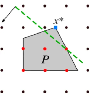
Example 2. Consider a simple integer program of just 2 variables,

max 1>x s.t. −2 6 2 1 x≤ 9 5 x∈_Z2 +. (1.3)

The feasible region of the linear programming relaxation of (1.3) is shown in Figure 1.1.

It is a polyhedron on the plane with vertices (0,0),(0,3/2),(3/2,2),(5/2,0). The linear

inequality 5x1 + 6x2 ≤ 16 does not eliminate any feasible integer points, therefore it is a

cut for (1.3). Furthermore, it cuts off the vertex x∗ = (3/2,2), and thus it is a violated

(13)

Figure 1.1: A cutting plane example

In fact, it turns out that the cut in Example 2 belongs to the family of split cuts

introduced by Cook et al. [25], which has shown to be the most useful family of cuts to

solve MIPs in practice [20]. We refer to [26] for a comprehensive review of several classical

families of cuts and how they are related to each other.

A central concept in the study of cutting planes is that of closures. In the next section, we give a brief overview of known results on closures.

1.2 Closures

To study the impact that a particular family of cuts may have, both theoretically and

com-putationally, a common approach is to consider the closure of those cuts. Given a family

of cuts, the associated closure is the convex set defined by the intersection of all cuts in the same family. Therefore, a closure can be seen as an approximation to the convex hull

of all feasible integer solutions, or simply, the integer hull. On the theoretical side, topics

range from determining polyhedrality of closures [25,45] and the complexity of optimizing a

linear function over them [23,32], to analyzing relationships between different closures [28]

and how well they approximate the integer hull [14]. On the computational front,

sev-eral authors proposed strategies to empirically evaluate the strength of different closures

by computing the amount of integrality gap (c.f. Definition 3) they close: we thus have

computational evaluations of the Chvátal closure [33], the split closure [13], the projected

Chvátal-Gomory closure [22], the MIR closure [29] and the lift-and-project closure [21].

Definition 3. Consider (1.1) and its linear programming relaxation (1.2). Suppose (1.1)

(14)

(1.1) and (1.2), respectively. Given a family of cuts. Let C denote its closure, and let

Opt_CLO := min

x∈C c >

x.

Then the integrality gap closed by C is expressed as the quantity

Opt_CLO−Opt_LP

Opt_{M IP} −Opt_LP.

Usually, integrality gaps are computed individually on a set of benchmark instances, and the average gap closed by a given family of cuts is then compared with others. The

Mixed Integer Programming LIBrary [4], or MIPLIB, is an electronically available library

consisting of various real-world pure and mixed integer programs. Currently MIPLIB has five versions. The first version was initiated in 1992, and the sixth version was just released on November 5, 2018. Since its introduction, MIPLIB has become a standard test set used to compare the performance of mixed integer optimizers. In this thesis we will use MIPLIB

3.0 [19] and MIPLIB 2003 [5], which are the third and the forth versions of MIPLIB. We

explain in more details about our choice of test sets in Chapter4.

The split closure, or equivalently the MIR closure, was shown computationally to be a

very tight approximation of the integer hull [13,36]. On average it closes more than 75%

of the integrality gap on MIPLIB 3.0 instances. This has since led to efforts on efficient

generation of strong split cuts (see, for example, [7,27,35,36]). We formally introduce split

cuts in the next section.

1.3 Split disjunctions and split cuts

Consider an integer vector π ∈ _Zn _where _π

j = 0 for all j ≥ p+ 1 and an integer π0 ∈ Z.

We define asplit disjunction forP ∩(_Zp_×

Rn−p)as

π>x≤π0 ∨ π>x≥π0+ 1. (1.4)

Note that (1.4) is satisfied by every x∈_Zp_×

Rn−p. Therefore, let Π(π,π0) 1 :=P ∩ {x∈R n _:_π> x≤π0}, Π(π,π0) 2 :=P ∩ {x∈R n :π>x≥π0+ 1}, (π,π ) (π,π)

(15)

Consider the convex hull of sets Π(π,π0) 1 and Π (π,π0) 2 P(π,π0) _:=_conv_Π(π,π0) 1 ∪Π (π,π0) 2 ,

where conv(S) denotes the smallest convex set that contains set S. Clearly x¯ ∈ P(π,π0)_.

We thus define split cuts as follows.

Definition 4. A split cutforP∩(_Zp_×

Rn−p)is a valid inequality for someP(π,π0)_{, where}

(π, π0) is a split disjunction forP ∩(Zp×Rn−p).

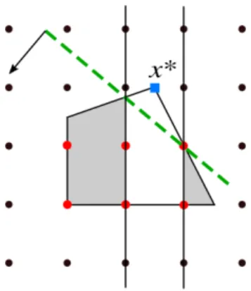
Example 5. The cut5x1+ 6x2 ≤16in Example2is a split cut corresponding to the split

disjunction π=

0 1

and π0 = 1, as illustrated in Figure 1.2.

Figure 1.2: A split disjunction and a split cut

Obtaining effective violated cutting planes for MIPs is usually a nontrivial process. The problem of finding a cut that separates a fractional point from the convex hull of all

feasible integer solutions, or showing that none exists, is called a Separation Problem. It

has been shown that the separation problem for split cuts is N P-hard [23] in general, and

costly in practice [36].

MIPs are hard to solve in general, but there is an important property that underlies many real-world problems and plays in our favor: sparsity. We discuss it in the next section.

(16)

(a) less structured (b) more structured

Figure 1.3: Examples of sparse matrices

1.4 Sparsity

In numerical analysis and scientific computation, a matrix or a vector is considered sparse

if most of the entires are zero, and it isdense if most of the entries are nonzero. Depending

on the contexts, the term sparsity has been used in the literature with different meanings

and emphases. Some authors refer to sparsity as the numeric quantity calculated from dividing the number of zero entries by the number of all entries, i.e., sparsity equals one minus density; some authors refer to sparsity as a general property of a matrix or vector being sparse. In this thesis, whenever we use the term sparsity, we mean the underlying matrix or vector is sparse. Sometimes the nonzero entries in a sparse matrix demonstrate

a clear pattern. This is illustrated in Figure 1.3, where we take two sparse matrices, both

have the same number of rows and columns, and plot their respective sparsity patterns by replacing each nonzero element with a black dot. Observe that most of the nonzero entries in the matrix on the right lie in five identifiable blocks, whereas the nonzero entries in the matrix on the left are distributed more arbitrarily. In fact, the more structured matrix in

Figure 1.3b is obtained from the less structured one in Figure 1.3a by permuting its rows

and columns. The advantage of having structured patterns in a sparse matrix will be made

clearer in Chapter 2.

In general, sparsity helps when storing and manipulating matrices and vectors on a computer, as specialized algorithms and data structures may be designed to take advantage of their sparse structures. During a MIP solution process, sparsity may be exploited in several ways. In the following we mention a few that motivate the goal in this thesis.

(17)

that are amenable to decomposition-based solution approach. A recent result of Bergner

et al. [15] shows that several benchmark instances have an almost block-diagonal structure

calledarrowhead, that is, a structure with several blocks that are linked only by few linking

variables and constraints (e.g. Figure1.3b). This shows that not only are these benchmark

instances sparse (on average, MIPLIB 2010 [42] instances only have 1.62% density), but in

many cases such sparsity has an identifiable structure that can be exploited.

Second, modern implementations of the simplex algorithm take advantage of sparsity

in solving large linear systems [47], an approach credited as one of the two most notable

improvements in the linear algebra routines of the simplex method [17]. Thus sparsity is a

desirable property of cutting planes for MIPs. Indeed, in almost every cut generation and selection procedure described in the articles we mentioned in the previous sections, specific heuristics were implemented to impose sparsity in the cuts, e.g., introducing a penalty

term in the objective of a cut generating problem to make the resulting cut sparser [33],

applying a coefficient reduction algorithm to reduce the number of nonzero coefficients in

the split cut [27], or discarding all dense cuts to ensure that only sparse cuts are added [35].

Additionally, in a recent computational study by Walter [48], it is shown that equivalent

but denser versions of the same cuts negatively affect the performance of MIP solvers. Due to all this interest, there has also been some recent work to analyze theoretically the

strength of sparse cutting planes [30,31].

Finally, in their computational study of the split closure [13], Balas and Saxena

ob-served that most split disjunctions they produced were sparse, regardless of problem size. Although sparse split disjunctions do not necessarily lead to sparse split cuts, the two are not uncorrelated. On the other hand, although split closure provides a tight approxima-tion to the integer hull, the time it takes to separate an arbitrary split cut makes it almost unrealistic to use in practice. Thus, given the possibility to exploit the sparsity underlying problem structures, and given the advantage of using sparser cuts, it is very interesting to evaluate the strength of split cuts based purely on sparse disjunctions, as a first step towards determining subsets of split cuts that are computationally more promising.

1.5 Motivations and outline

Split cuts have been shown to be strong theoretically—they dominate Chvatál-Gomory

cuts, even on pure-integer sets [25]—and computationally [13,29,36]. Furthermore, even

small subfamilies of split cuts, namely GMI and MIR cuts from tableaux, have proven

extremely invaluable in practice [20]. On the other hand, finding a general split cut is hard

(18)

beyond GMI and MIR cuts from tableaux, with promising computational properties. The main goal of this thesis is to study the strength of split cuts that exploit sparsity. Our contributions are the following. First, we implement an approximate separation

rou-tine based on the work on Balas and Saxena [13] that separates only split cuts whose split

disjunctions are sparse and whose split coefficients are small. Second, we show empirically that in spite of these restrictions, the integrality gap closed by this subclass of split cuts is still quite significant compared to gap closed by the full split closure. Finally, we consider problem structures of individual instances and show that split cuts computed by

consider-ing only constraints and variables from a sconsider-ingle block in anarrowhead decomposition[15,37]

of the constraint matrix also largely preserve the strength of general split cuts, in terms of gap closed.

The focus of this work is computational, but the tools and results should be interesting to both practitioners and theoreticians. For example, although the separation problem

for general split cuts is N P-hard, finding a split cut arising from split disjunction with

just one nonzero entry can be done in polynomial time [21]. Therefore, one might ask,

how hard is it to optimize over all split cuts arising from split disjunction with support that has cardinality at most, say, two, five, ten? Furthermore, to begin with, is it even a meaningful question to think about? The results that we present in this thesis provide a positive answer: Split cuts from sparse disjunctions constitute a strong subclass of split cuts and indeed worth further study, both computationally and theoretically.

This thesis is organized as follows. In Chapter 2 we give a quick introduction to the

cut generating linear program and the cut lifting procedure that are necessary for our

separation routine. Then we lay out the basic approach of Balas and Saxena [13] for the

separation of split cuts. Finally we introduce the automatic arrowhead decomposition of

Bergner et al. [15]. In Chapter3we detail the implementation of our split cut separator. In

particular, we describe exactly what measures we took to obtain cuts that are numerically

stable and effective, while being verifiably valid. Chapter 4 presents the results of our

(19)

Chapter 2 Background

In this chapter we review some basic results in linear and integer programming that will enable us to develop from first principles an approximate split cut separator for general MIPs. In particular, we begin by introducing the so-called Cut Generating Linear Program for split cuts, of which one variant plays a key role in our separator. Then we discuss a classical idea, called lifting, to obtain a cutting plane valid for a higher dimensional polyhedron from a given cutting plane valid for a lower dimensional one. It turns out that the lifting procedure significantly reduces computation time in practice and, as a result, makes the separation of split cuts realistic. With these basic technical tools, we present

details of the approach of Balas and Saxena [13] for the separation of split cuts. Lastly,

we give a concise overview of the method of Bergner et al. [15] to automatically detect

structured sparsity in MIP instances.

2.1 Cut generating linear program

The idea that one can formulate the problem of finding a cutting plane valid for some given polyhedron as a linear program relies on Farkas’ lemma. Farkas’ lemma provides a simple characterization about the solvability of a system of linear inequalities. In the following we state three versions of Farkas’ lemma that will be useful in our context. Proofs of Farkas’

lemma can be found in various introductory texts, e.g., [24, Theorem 3.4] and [16, Theorem

4.6].

Theorem 6 (Farkas’ lemma). LetA∈_Rm×n _and _b_∈

Rm. Then

x∈_Rn :Ax≤b =∅ ⇐⇒

(20)

Corollary 7 (Farkas’ lemma, other versions). Let A ∈ _Rm×n_{, G} _∈ Rl×n, b ∈ Rm, d ∈ Rl. Then x∈_Rn _:_Ax₌_{b, x}_≥₀ ₌_∅ _⇐⇒ u∈_Rm _:_A> u≤0, b>u >0 6=∅, and x∈_Rn:Ax=b, Gx≥d, x≥0 =∅ ⇐⇒ (u, v)∈_Rm_× Rl:A>u+G>v ≤0, b>u+d>v >0, v ≥0 6=∅.

Here is a direct consequence of Farkas’ lemma.

Corollary 8. Suppose P ={x∈_Rn_: _Ax₌_{b, x}_≥₀_{} 6}₌_∅_{, and} _min_{_c>_x_:_x_∈_P_}_>_−∞_.

ThenD={y∈_Rm _:_A>_y_≤_c_{} 6}₌_∅_.

Proof. IfD=∅, then by Farkas’ lemma, there isu¯∈_Rn_{such that} _A¯_u_{= 0, c}>_{u <}_¯ _0,_u_¯_≥₀_.

Letx¯ ∈P, then x¯+λ¯u ∈P for all λ≥ 0, and limλ→+∞c>(¯x+λ¯u) =−∞, contradicting

to our assumption thatmin{c>x:x∈P}>−∞.

Another useful result in linear programming is strong duality.

Theorem 9 (Strong duality). Let P = {x ∈ _Rn _: _Ax ₌ _{b, x} _≥ ₀_} _and _D ₌ _{_y _∈

Rm :

A>y ≤ c}. If P =6 ∅ and D6= ∅, then min{c>x :x ∈ P}= max{b>y :y ∈ D}, and there

exist x∗ ∈P and y∗ ∈D such that c>x∗ =b>y∗.

Recall that an inequality α>x≥β is a valid split cut corresponding to the disjunction

(π, π0)only if it is satisfied by all points inP(π,π0) =conv Π

(π,π0) 1 ∪Π (π,π0) 2 , whereΠ(π,π0) 1 = P ∩ {x:π>x≤π0}, Π (π,π0) 2 =P ∩ {x:π >_x_≥_π 0+ 1}, and P ={x∈Rn :Ax =b, x≥0}.

Farkas’ lemma enables us to certify the validity ofα>x≥β relative toP(π,π0)_{, as stated in}

Theorem 10. We give a proof that is similar to the proof of Theorem 3.22 in [24]. However,

we note that the statement of Theorem 3.22 in [24] does not extend completely trivially to

Theorem 10 that we present here. The slight technicality comes when one of Π(π,π0)

1 and

Π(π,π0)

(21)

Theorem 10. Suppose P(π,π0) ₆₌ _∅_{. An inequality} _α>_x _≥ _β _{is valid for} _P(π,π0) _{if and}

only if there exist y, z ∈ _Rm_, _{s, t} _∈

Rn, y0, z0 ∈ R, such that s, t ≥ 0, y0, z0 ≥ 0, and the

following conditions hold:

α=A>y+s−y0π

α=A>z+t+z0π

β≤b>y−y0π0

β≤b>z+z0(π0+ 1).

(2.1)

Proof. Since P(π,π0) ₆₌ _∅_{, we may assume without loss of generality that} _Π(π,π0)

1 6= ∅.

Our proof considers Π(π,π0)

1 and Π (π,π0)

2 separately. The required result follows by simply

observing that if α>x ≥ β is valid for both Π(π,π0)

1 and Π (π,π0)

2 , then it must be valid for

P(π,π0)_{, too.}

Let us first show that α>x ≥ β is valid for Π(π,π0)

1 if and only if there exist (y, y0) ∈

Rm×R and s ∈Rn such that

α=A>y+s−y0π, β ≤b>y−y0π0, s≥0, y0 ≥0. (CRT-1)

Supposeα =A>y+s−y0π and β ≤b>y−y0π0 for some (y, y0)∈Rm×R ands ∈Rn

such that s≥0 and y0 ≥0. Then for all x∈Π

(π,π0)

1 ,

α>x = y>Ax+s>x−y0π>x = y>b+s>x−y0π>x

≥ y>b−y0π>x ≥ y>b−y0π0 ≥ β.

Conversely, suppose α>x≥β is valid for Π(π,π0)

1 . Consider the linear programs

min α>x s.t. Ax =b π>x+x0 =π0 x≥0, x0 ≥0 (P) max b>y+π0y0 s.t. A>y+πy0 ≤α y0 ≤0 (D).

The feasible region of (P) is (x, x0) ∈ Rn ×R : x ∈ Π

(π,π0)

1 , and thus is nonempty.

Furthermore, since α>x ≥β is valid for Π(π,π0)

1 , (P) has a finite optimum β

∗ _≥_{β >} _−∞_.

By Corollary8, the feasible region of (D) is nonempty. Therefore, by strong duality, there

(22)

but upon flipping the sign of y0 and adding slack variables s ≥ 0, this is exactly the

condition (CRT-1).

Let us now consider Π(π,π0)

2 . The conditions that α>x ≥ β is valid for Π

(π,π0)

2 if and

only if there exist (z, z0)∈Rm×R and t∈Rn such that

α=A>z+t+z0π, β ≤b>z+z0(π0+ 1), t≥0, z0 ≥0 (CRT-2)

follows analogously if Π(π,π0)

2 6= ∅. So suppose Π

(π,π0)

2 = ∅. By Farkas’ lemma applied to

Π(π,π0)

2 , there exist (u, u0)∈Rm×Rsuch that

A>u+πu0 ≤0, b>u+ (π0+ 1)u0 >0, u0 ≥0.

Note that we must haveu0 >0(otherwise, by Farkas’ lemma, we would get a contradiction

to P 6= ∅, and thus contradicting P(π,π0) ₆₌_∅_{). But then for any} _{(y, y}

0) and s that satisfy

(CRT-1) and any appropriately scaled(u, u0) such that

b>u+ (π0+ 1)u0 ≥y0 and u0 ≥y0,

we obtain (z, z0) and t that satisfy (CRT-2) by setting

z :=y+u, z0 :=u0−y0 ≥0, t:=s−A>u−πu0 ≥0.

This completes the proof.

Remark 11. As noted in [34], for technical reasons we usually assume that the trivial

inequality0>x ≥ −1 is contained (implicitly) in the system Ax = b, x ≥0 that describes

the constraint set. For problems with at least one bounded variable, say lj ≤ xj ≤ uj,

such trivial inequality may be obtained by addingxj ≥lj and−xj ≥ −uj and dividing the

resulting inequality by uj −lj > 0. Due to the presence of 0>x ≥ −1, we are allowed to

require the ≤inequalities for β in Theorem 10to hold at equality. We will therefore make

such an assumption in all of our subsequent discussions.

Theorem 10immediately allows us to check whether a point xˆ∈P lies in P(π,π0)_.

Corollary 12. Letxˆ∈P. Then xˆ∈P(π,π0) _{if and only if the following optimization}

(23)

value. min α>xˆ−β s.t. α=A>y+s−y0π α=A>z+t+z0π β =b>y−y0π0 β =b>z+z0(π0+ 1) y, z ∈_Rm_{, s, t}_∈ Rn+, y0, z0 ∈R+ (CGLP(π, π0))

Therefore, given a point xˆ ∈ P and a split disjunction (π, π0) ∈ Zn×Z, a most

vio-lated split cutα>x≥β can be obtained by solving the corresponding (CGLP(π, π0)). The

optimal objective value is negative if such a cut exists. Otherwise, (CGLP(π, π0)) proves

ˆ

x∈P(π,π0)_.

Remark 13 (Normalization). The objective value of (CGLP(π, π0)) is unbounded from

below when it has a negative objective value. This is because one can scale up the solutions

(α, β, y, z, s, t, y0, z0) while maintaining feasibility. In other words, the feasible region of

(CGLP(π, π0)) is a cone. Therefore, a normalization constraintf(α, β, y, z, s, t, y0, z0) =κ,

where κ is a positive constant normally set to be 1, is introduced to truncate the cone of

feasible solutions. Many choices off are possible, for example,

• β-normalization [11] f(·) :=β or f(·) :=−β; • α-normalization [11] f(·) := n X j=1 |αj|; • trivial normalization f(·) :=y0+z0; • standard normalization [10] f(·) := m X j=1 |yj|+ m X j=1 |zj|+ n X j=1 sj + n X j=1 tj +y0+z0;

(24)

• Euclidean normalization [34] f(·) := m X j=1 kAjk|yj|+ m X j=1 kAjk|zj|+ n X j=1 sj+ n X j=1 tj +kπky0+kπkz0

where Aj is the jth column of A and k · k is the Euclidean norm of a vector.

Normalization methods directly affect the quality of cut coefficientsαandβ as solutions of

(CGLP(π, π0)). The conditions of interest in our context are the trivial and the standard

normalization conditions. The former is simple enough to make the separation of arbitrary

split cuts possible, and the latter usually produces stronger cuts [34] and is used in our

setting as a heuristic strengthening procedure for split cuts. We will return to this in

Chapter 3.

We refer to [11,12,34] for in-depth discussions of different normalization conditions.

The following observation on the nonnegativity of Farkas’ multipliersyandzin (CGLP(π, π0))

is useful when imposing normalization conditions. It allows us to avoid unnecessary

lin-earization of the absolute value constraint on y and z. While, in the literature, previous

works use this observation as a fact, we couldn’t find any proof. Here, we give a proof for the sake of completeness.

Proposition 14. Letxˆ∈P. If (CGLP(π, π0)) has an optimal solution under the trivial,

standard, or Euclidean normalization condition, then it has an optimal solution in which

the Farkas’ multipliersy and z are nonnegative.

Proof. Let( ˆα,β,ˆ y,ˆ z,ˆ ˆs,t,ˆyˆ0,zˆ0)be an optimal solution to (CGLP(π, π0)) under

normaliza-tionf(·), wheref(·)belongs to one of the conditions in the statement. Defineˆc∈_Rm _such

that ˆ cj :=        0 if yˆj ≥0and zˆj ≥0, −yˆj if yˆj <0 and zˆj ≥0, −zˆj if yˆj ≥0and zˆj <0, −yˆj −zˆj if yˆj <0 and zˆj <0. and consider α:= ˆα+A>cˆ β := ˆβ+b>cˆ y:= ˆy+ ˆc z := ˆz+ ˆc, s:= ˆs, t := ˆt, y₀ := ˆy0, z0 := ˆz0.

(25)

(i) |y_j|+|zj|=|yˆj|+|zˆj| for all j = 1,2, . . . , m;

(ii) α>xˆ−β = ˆα>xˆ−βˆ;

(iii) y ≥0and z ≥0.

The proof is completed by noting that (i) gives feasibility of (α, β, y, z, s, t, y₀, z0) under

the same normalization f(·) = κ; (ii) gives optimality; and (iii) gives nonnegativity as

required.

As a result of Proposition 14, we will require that y ≥ 0 and z ≥ 0 in (CGLP(π, π0))

from now on.

2.2 Cut lifting

Lifting is a classical topic in integer programming, whose origin dates back to the 1960’s

and 70’s in the contexts of the group problem [39] and the set packing problem [44]. A

lifting problem can be stated as follows:

We are given I ⊆ {1,2, . . . , n}, P =x∈_Rn :Ax =b, x≥0 , Q=x∈P :xj ∈Z, ∀j ∈ I , PR= xR ∈_Rn−q _: xR 0 ∈P , QR=xR ∈PR :x_jR∈_Z, ∀j ∈ I ∩ {1,2, . . . , n−q} , (2.2)

i.e., PR is the restriction of P obtained by setting the last q variables to 0. Given an inequality αR>

xR _≥ _β _{valid for} _QR_{, find} _α _∈

Rn such that α>x ≥ β is valid for Q and αj =αRj for 1≤j ≤n−q.

When trying to obtain a split cut that separates xˆ∈ P fromQ, a usual strategy is to

work in the subspace, say_Rn−q_{, of variables} _x_ˆ

j that are not at their bound (i.e., xˆj > 0),

find a cut αR)>x ≥ β in _Rn−q, and then lift it to _Rn. Note that since x ≥ 0 for every

x∈P, we would like the lifted coefficients as small as possible, in the sense that the lifted

cut is potentially stronger. Therefore, an approach is to minimize cut coefficients subject to the lifted cut remaining valid. We give the details below.

(26)

A trivial lifting procedure for split cuts:

SupposeP, Q, PR, QRare as in (2.2). Given a pointxˆ∈P such that, up to permutation

of indices, xˆj > 0 for 1 ≤ j ≤ n−q and xˆj = 0 otherwise. Then the projection xˆR of xˆ

onto _Rn−q _{lies in} _PR_{. Given} _(αR_{, β)}_∈

Rn−q×R such that

(i) (αR)>xˆR < β;

(ii) (αR₎>_xR _≥ _β _{is a split cut for} _PR _{corresponding to a split disjunction} _(πR_{, π}

0) ∈

Zn−q×Z.

Our goal is to obtainα ∈_Rn _{such that}_α

j =αRj for 1≤j ≤n−q and

(i’) α>x < βˆ ;

(ii’) α>x ≥ β is a split cut for P corresponding to a split disjunction (π, π0) ∈ Zn×Z

where πj =πjR for 1≤j ≤n−q and πj = 0 for n−q+ 1≤j ≤n;

(iii’) αj is minimized for n−q+ 1 ≤j ≤n.

Note that, in the above,(ii) implies(αR)>xR≥β is valid forQRand (ii’)impliesα>x≥β

is valid forQ. The following Theorem15is a straightforward extension of the trivial lifting

procedure of lift-and-project cuts described in [11].

Theorem 15. Given (αR_{, β)} _{that satisfies} _(i) _and _(ii)_{. Let} _AR _∈

Rm×(n−q) be obtained

fromAby removing the lastqcolumns. LetyR∈_Rm_{, z}R_∈

Rm, sR∈Rn−q, tR∈Rn−q, y0R∈ R, z0R ∈Rsatisfy αR = (AR)>yR+sR−y₀RπR= (AR)>zR+tR+z₀RπR, β =b>yR−y₀Rπ0 =b>zR+z0R(π0+ 1), yR, zR, sR, tR, yR₀, zR₀ ≥0. (2.3)

Define α∈_Rn _{such that} _α

j =αjR for 1≤j ≤n−q and

αj = max

A>_jyR, A>_j zR , n−q+ 1≤j ≤n, (2.4)

where Aj is the jth column of A. Then (α, β) satisfies (i’) and (ii’). Furthermore, if the

(27)

Proof. Note that (i’) is always satisfied since xˆj = 0 for n−q+ 1 ≤ j ≤ n. To see that

(ii’) is satisfied, observe thatα satisfies

αj =αRj, 1≤j ≤n−q, αj ≥A>j y R_, _n₋_q_{+ 1} _≤_j _≤_n, αj ≥A>j z R_, _n₋_q_{+ 1} _≤_j _≤_n, (2.5)

and (yR, zR)satisfies (2.3). The validity ofα>x≥β corresponding to the split disjunction

(π, π0) defined in(ii’) follows directly by applying Theorem10.

If the multipliers (yR, zR) that satisfy (2.3) are unique, then the lifted cut α>x ≥β is

valid if and only if (2.5) holds, and thus αj is minimized by taking the maximum of A>jyR

and A>_jzR_.

Remark 16. It is clear from our construction in this section that, given xˆ∈P, there is a

split cutα>x≥β forP that corresponds to disjunction (π, π0)and cuts offxˆif and only if

there is a split cut(αR₎>_xR _≥_β _for _PR _{that corresponds to disjunction} _(πR_{, π}

0)and cuts

off xˆR_.

Remark 17. There is no loss of generality in assuming that the feasible region of every

MIP is of the form Q. Indeed, for a free variable xj we can replace it with two bounded

variablesx+_j andx−_j such thatxj =x+j −x

−

j . For a bounded variablexj with nonzero lower

bound lj and upper bound uj, we can do either of the following:

• shift the lower bound, i.e., replace b with b−ljAj, then subsume the upper bound

into constraints Ax =b; or

• complement the variable and shift the upper bound, i.e., replace Aj with −Aj and

replace b with b−ujAj, then subsume the lower bound into constraints Ax=b.

Of course, we can always require inequality constraints to hold at equality by adding slack variables.

Following Remark17, the lifting procedure described here easily extends to MIPs whose

variables have nonzero lower and/or upper bounds. In practice, depending on a given xˆ,

for each bounded variable xˆj we choose one of the transformations in Remark 17so that,

(28)

2.3 Optimizing over the split closure

The split closure SC for mixed-integer set P ∩(_Zp∩_Rn−p₎_{is defined as}

SC= \

(π,π0)∈Zn×Z

πj=0, j≥p+1

P(π,π0)_.

Givenxˆ∈P, the problem of deciding wetherxˆ∈ SCisN P-hard in general [23]. Balas and

Saxena [13] implemented an iterative procedure that alternates between a Master Problem

and aSeparation Problem to find

min{c>x:x∈ SC}.

At each iteration, the Master Problem is a linear program of the form

min{c>x:x∈P, αtx≥βt, t∈T} (MP)

where {αtx ≥βt : t ∈T} is the set of all split cuts generated by the Separation Problem

so far. If xˆ is an optimal solution to (MP), the Separation Problem then finds a valid

split cut violated byxˆ, or proves thatxˆ∈ SC. The Separation Problem is a mixed-integer

nonlinear program obtained from (CGLP(π, π0)) with trivial normalization y0 +z0 = 1,

and allowing(π, π0)to vary over Zn×Z, written as:

min α>xˆ−β s.t. α=A>y+s−y0π α=A>z+t+z0π β =b>y−y0π0 β =b>z+z0(π0 + 1) 1 = y0+z0 y, z ∈_Rm +, s, t∈R n +, y0, z0 ∈R+ (π, π0)∈Zn×Z, πj = 0, j ≥p+ 1. (SP)

In [13], (SP) is shown to be equivalent to a parametric MILP with a scalar parameter

taking values between 0 and 1₂. For completeness we state and prove their result here.

Theorem 18 ( [13]). The optimum of (SP) is equal to the optimum of the following

parametric mixed-integer linear program,

(29)

where each MILP(θ) is given by min s>xˆ−θ(π>xˆ−π0) s.t. A>w+s−t−π = 0 b>w−π0 = 1−θ w∈_Rm, s, t∈_Rn₊ (π, π0)∈Zn×Z, πj = 0, j ≥p+ 1. (MILP(θ))

Proof [13]. Apply the following modifications to (SP):

(a) substitute α=A>y+s−y0π and β =b>y−y0π0 into the objective;

(b) eliminate α and β from the constraints;

(c) substitute z0 = 1−y0 into the constraints;

(d) replace y−z with w and replacey0 with θ.

We see that (SP) is equivalent to

min

0≤θ≤1MILP(θ).

Now, fix θ = ˆθ and suppose ( ˆw,s,ˆ t,ˆπ,ˆ πˆ0)is a feasible solution for MILP(θˆ). Then

w:=−w,ˆ s:= ˆt, t := ˆs, π:=−π,ˆ π0 :=−πˆ0−1

is a feasible solution for MILP(θ) with θ:= 1−θˆ, and that

s>xˆ−θ(π>xˆ−π0) = ˆt>xˆ−(1−θ)(ˆ −πˆ>xˆ+ ˆπ0+ 1)

= ˆt>xˆ+ ˆπ>xˆ−πˆ0−1 + ˆθ−θ(ˆˆπ>xˆ−πˆ0)

= ˆs>xˆ−θ(ˆˆπ>xˆ−πˆ0),

where the last line follows from ˆs>xˆ= ˆt>xˆ+ ˆπ>xˆ−πˆ0 −1 + ˆθ, which in turn is obtained

as a linear combination of constraints in MILP(θ)ˆ, i.e.,

ˆ x> A>wˆ+ ˆs−tˆ−πˆ− b>wˆ−πˆ0 =−1 + ˆθ. Therefore, min

0≤θ≤1MILP(θ)= min0≤θ≤1MILP(1−θ)= min0≤θ≤1₂

(30)

We immediately obtain a result similar to that of Corollary 12.

Corollary 19. Letxˆ∈P. Thenxˆ∈ SC if and only if

min

0≤θ≤1 2

MILP(θ)≥0.

Writing (SP) as a parametric mixed-integer program enables us to approximate its

optimum by solving a finite sequence of problems MILP(θ) with varying values for θ using

state-of-the-art MIP solvers.

2.4 Automatic detection of double-bordered block-diagonal

structure

The idea of exploiting block-diagonal structure in sparse matrices has been widely dis-cussed in the contexts of numerical linear algebra and mathematical programming. One motivation is that the diagonal blocks usually give rise to small independent subproblems well suited for parallel processing. Applications include solving systems of linear equa-tions arising from a discretization of a continuous domain, LU and QR factorizaequa-tions, and decomposition-based solution methods for structured (mixed-integer) linear programs. In

general, the constraint matrix Aof (1.1) does not admit a block-diagonal form, but it can

be put into a k-waydouble-bordered block-diagonal form

       D1 _F1 D2 F2 . .. .._. Dk Fk A1 _A2 _{· · ·} _Ak _G        (DB-k)

for some k ≥1. This is sometimes informally called the arrowhead form. The constraints

associated with rows in Ai are called linking constraints, and the variables associated with

columns in Fi _{are called} _{linking variables}_.

Given a sparse matrix, Aykanat et al. [8] considered the problem of obtaining a DB-k

form by permuting its rows and columns. They reduce the matrix permutation problem

(31)

blocks is fixed, computational experiments show that the resultingDB-k forms demonstrate significant variability and are very sensitive to input parameters. To cope with this, Bergner

et al. [15] proposed to use a proxy measure to automatically detect the “best” DB-kform, for

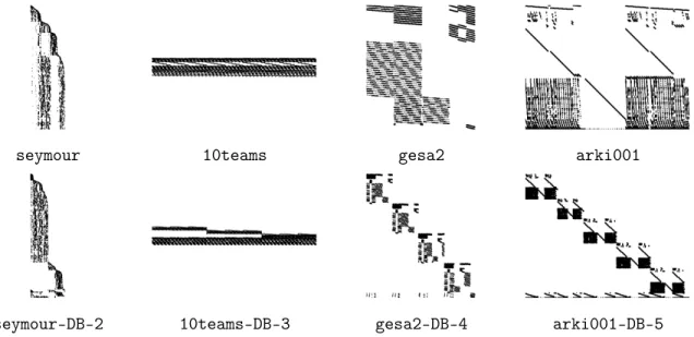
the purpose of applying Dantzig-Wolfe reformulations to general MIPs. Figure 2.1 shows

a few examples of MIPLIB instances, with black dots representing nonzero coefficients of the constraint matrix. The bottom row shows a rearrangement of the columns/rows of the

matrix evidencing theDB-k structure.

seymour 10teams gesa2 arki001

seymour-DB-2 10teams-DB-3 gesa2-DB-4 arki001-DB-5

(32)

Chapter 3 Implementation Details

In this chapter we outline the computational details in our implementation of a split cut

separator with (and without) structural information supplied by a given DB-k form. We

follow the idea of Balas and Saxena [13] to approximate the optimal value of (SP) by solving

a sequence of (MILP(θ))’s parametrized byθ ∈[0,1/2]. The structure of this chapter is as

follows. We begin by introducing some practical methods used in our implementation that

are taken from or similar to those already presented in [13]. Then we discuss new features

that we added to serve our goal of evaluating split cuts based on sparsity properties. Finally we lay out concise algorithmic descriptions of the entire computational process.

3.1 Existing methods for practical computation

Discretizing parameters. We denote byΘthe set of values ofθ for which (MILP(θ))

will be solved. By Theorem 18, obtaining an exact solution of (SP) would require that

Θ = [0,1/2], which is prohibitive in practice. Therefore, we takeΘas a uniform parameter

grid of finitely many points between 0and 1/2. The initial size of Θis t, and we increase

the number of grid points whenever necessary, following the criteria in Algorithm1.

Stabilizing objective. When some entries in an incumbent solution xˆ are close to

their bounds, sayxˆj ≈0 for j ∈ J, the objective coefficients for s in (MILP(θ)) are close

to zero. As a result, there may exist multiple feasible solutions(w, s, tπ, π0)with differing

valuessj andtj forj ∈ J, whose objective values are arbitrarily close to optimum. Some of

these sj’s and tj’s can be unnecessarily large, which in turn leads to weak split directions

(33)

happen. First, a split disjunction may be “squeezed” as its coefficients simultaneously become large, the two sides of the disjunction get close to each other in Euclidean norm, and thus we are not cutting off many points. Second, a split disjunction may be “tilted” away from the disjunction that produces most violated cut, and thus leading to weaker

cuts. We illustrate this latter observation in Example 20.) However, due to numerical

tolerances in a MIP solver, these poorly-scaled suboptimal solutions may be regarded as

optimal. Therefore, to avoid obtaining unnecessarily weak cut coefficients, we replacexˆin

the objective of (MILP(θ)) with

˜

xj := max{xˆj, δ}, ∀j,

for δ a small positive constant. We show the effect of this modification in a concrete

ex-ample.

Example 20. Consider the integer program from Example2. Let us write it in the general

form of (1.1) by adding 2 continuous slacks variablesx3 andx4. Given a point x0 ∈R4, we

may find a split disjunction (π, π0)∈Z4×Z and a split cut that separates x0 from P(π,π0)

by substituting the data into (MILP(θ)),

min 4 X j=1 x0_jsj −θ 4 X j=1 x0_jπj+θπ0 s.t. π=     −2 2 6 1 1 0 0 1     w+s−t π0 = 9 5 w−1 +θ wfree, s, t ≥0 (π, π0)∈Z4×Z, π3 =π4 = 0 (3.1)

and solve it for someθ ∈[0,1/2]. Suppose we want to separate

x0 = (0.000000001, 1.5, 0.000000002, 3.499999998)>.

Takeθ = 1/10. It is easy to verify that

w0 = ₂₁₀ 31 4 35 , s0 =     1 15 0 0 0     , t0 =     0 0 210 31 4 35     , π0 =     0 1 0 0     , π₀0 = 1 (3.2)

(34)

is an optimal solution for (3.1) with optimal objective value − 749999999

15000000000 ≈ −0.049999. We

thus recover(α, β) from(s0, t0, π0, π₀0) as

α=s0−θπ0 =     1 15 −1 10 0 0     , β =−θπ0 =− 1 10.

Sincex3 = 9 + 2x1−6x2 andx4 = 5−2x1−x2, we can eliminate cut coefficients for slack

variables (in this case they are already 0) and obtain a cut in the space of (x1, x2) as

1 15x1− 1 10x2 ≥ − 1 10.

However, solving (3.1) with the same x0 and θ = 1/10 by CPLEX 12.71 we obtained a

solution w00≈ −23333279 210 4 35 , s00 ≈     0 0 23333279 210 0     , t00≈     18333329 15 0 0 4 35     π00 =     −1000000 −666665 0 0     , π₀00=−999998 (3.3)

whose objective value is approximately−0.049678. After eliminating slack variables, (3.3)

gives the cut

322221.70476x1−599998.61428x2 ≥ −899997.87142.

We note that lower bounding the objective coefficients by some appropriate δ, for example

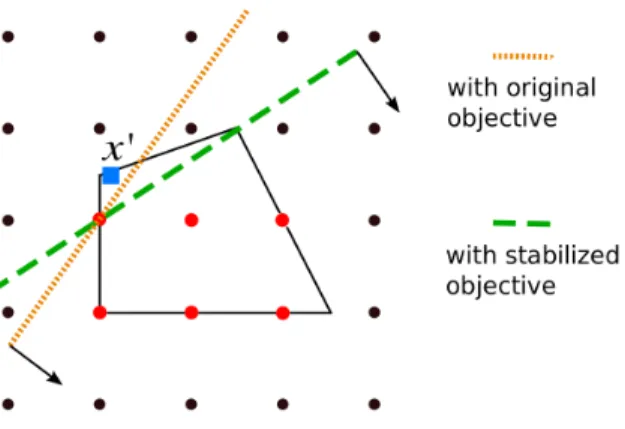
δ = 0.0001, helped CPLEX find the optimal solution (3.2). Figure 3.1 shows the cuts

obtained from CPLEX by solving (3.1) with and without our stabilizing objective.

Cut strengthening. Once a feasible solution ( ¯w,s,¯ ¯t,π,¯ π¯0) for MILP(θ¯) with a

neg-ative objective value is found, we feed (¯π,π¯0) into (CGLP(π, π0)) with the standard

nor-malization m X j=1 yj + m X j=1 zj + n X j=1 sj+ n X j=1 tj +y0+z0 =κ

(35)

Figure 3.1: Effect of stabilizing objective

Cut lifting. We work in the subspace of the variables that are not at their bounds

in the incumbent solution, and lift the resulting cuts to the full space following the lifting

procedure described in Chapter2.

Set covering. In an effort to impose some degree of orthogonality in the set of split

disjunctions, every time a split (¯π,π¯0) is found, we solve the set covering problem

min z∈{0,1}p ( _p X j=1 min{xˆj − bxˆjc,dxˆje −xˆj}zj : p X j=1 I[πj6=0]zj ≥1,∀π∈ S ) (StCvIP(ˆx,S))

where S is the set of splits already discovered, and _I[k6=0] = 1 if k 6= 0, I[k6=0] = 0 if

k = 0. Let zˆ be an optimal solution to (StCvIP(ˆx,S)), then we impose πj = 0 for all

j ∈ {j : ˆzj 6= 0} when solving (MILP(θ)) in the next θ point. This modification ensures

that (MILP(θ)) never returns a split disjunction whose support is identical to that of an

already discovered one. In practice it also prevents us from obtaining the same π with

varying θ values, which is an important property that makes our implementation more

effective. Moreover, we observed that the computation time spent on solving set covering

problems is almost negligible compared to the time spent on solving (MILP(θ)).

3.2 New features in our implementation

In addition to some modifications of (MILP(θ)) described in the last section, we added three

more constraints to (MILP(θ)) in order to control the quality and structural properties of

(36)

Fractionality constraint. Split disjunctions (π, π0) where π>xˆ is too close to either

π0 or π0+ 1 usually give rise to weak split cuts. To avoid that, we impose the bounds

σ≤π>xˆ−π0 ≤1−σ (C1)

for a smallσ >0.

Sparsity constraint. To impose the condition thatπis sparse with at mostM nonzero

entries, we introduce binary variablesr ∈ {0,1}p _{and constraints}

−U rj ≤πj ≤U rj, ∀j = 1, . . . , p, and

p

X

j=1

rj ≤M (C2)

whereU is an artificial upper bound on the magnitude of the components of π. Note that

imposing an artificial upper and lower bound on disjunction coefficients not only helps us control the sparsity, but also prevent us from obtaining weak splits due to unnecessarily large disjunction coefficients.

Structure constraint. Given a DB-k form of the constraint matrix A, to compute

split disjunctions whose support lie entirely in a single block Di_{, we simply impose that:}

πj =sj =tj = 0, ∀j 6∈ Ci

wj = 0, ∀j 6∈ Ri

(C3)

whereCi _and _Ri _{are column and row index set of} _Di_{, respectively.}

Certifying validity. For every split cut α>x ≥β generated from (CGLP(π, π0)), we

provide another certificate for the validity of the cut. Let ˆ βl := min x∈P{α > x:π>x≤π0} and βˆu := min x∈P{α > x:π>x≥π0+ 1}.

Then it should always hold that β ≤ min{βˆl,βˆu}. If the inequality fails, then the cut is

invalid and we discard it. In theory, split cuts returned by (CGLP(π, π0)) should always be

valid as they are obtained from Farkas multipliers which already certify their validity; in practice, however, we may obtain invalid cuts due to either a numerical issue within the LP or MIP solver or an error in our own implementation. Having an independent procedure that checks the validity of cuts before adding them to the Master Problem ensures our computational results are reliable, in the sense that as long as our checker implementation is correct, not a single invalid cut is added during the entire computation.

(37)

greatest absolute value of cut coefficients equals104_{. Furthermore, after scaling we set all}

cut coefficients whose absolute value is less than10−6 to zero. In general, setting a nonzero

cut coefficient to zero may strengthen the cut and make it invalid, but since our tolerance is small, the effect is small as well. Nonetheless, the validity of the cut is always subsequently certified by the independent checker. Note that this scaling process also serves as an implicit dynamism control, i.e., the ratio between the greatest and the smallest absolute

value of cut coefficients is no greater than1010_.

Time limit on the MIP solver. Mixed-integer linear programs are much harder

to solve than linear programs in general. As a result, even finding a feasible solution to

(MILP(θ)) can be extremely time-consuming. We observed that this is frequently the

case, in particular, when separating a point that is close to the closure we aim to optimize over. Therefore, a deterministic time limit of 800 ticks (roughly 1 second) is set for each

(MILP(θ)) we process. We use CPLEX’s deterministic time (ticks) so that the results are

reproducible and comparable across different machines.

Dynamics. At each iteration, if no cut is generated because we could not find a feasible

solution to (MILP(θ)), we increase the time limit to 48,000 ticks (roughly 60 seconds) and

the upper cutoff limit of the objective value. If there is no improvement in the optimal

objective value of the (MP) for a while (see Algorithm 1), we increase the number of grid

points and add more cuts per iteration. Furthermore, in order to control the number of cuts presented in the Master Problem, we delete all cuts that are nonbinding in the incumbent solution every five iterations.

Global time limit. The whole process is terminated if the entire computation time

exceeds a global time limit.

3.3 Algorithmic descriptions

Details of the iterative procedure are described in Algorithm1. The cut generation

(38)

Algorithm 1: Overall cut generation loop

1 Initialization.

Choose initial parameter grid sizet, upper objective value cutoff limits γ1 < γ2 <0,

deterministic time limits τ1 =800 ticks, τ2 =48,000 ticks. Set iteration counter

Iter=0. Denote k the number of blocks in a givenDB-k from; if no decomposition

is available, set k= 1.

2 TimeLimit←τ1, Cutoff ←γ1.

3 Iter← Iter + 1. Solve (MP) and obtain optimal solution xˆ. Denoten the number

of consecutive iterations where no improvement in the optimal objective value is made. Delete nonbinding cuts if necessary.

4 if n = 100 then return xˆ.

5 Update parameter grid size in the current iteration.

if 0≤n≤39 then s←2b0.1nc_t_. _else _s_←_16t_.

6 Set parameter grid Θ uniformly with|Θ| ←s.

7 Separation.

for j = 1, . . . , k do Generate a set K(j) _{of cuts following}

CutGen(ˆx,Θ,Cutoff,TimeLimit)for block j.

8 if Sk_j₌₁K(j)6=∅ then Add cuts to (MP),go to 2.

9 else if TimeLimit= τ₁, Cutoff= γ₁ then TimeLimit←τ₂, go to 7.

10 else if TimeLimit= τ2, Cutoff= γ1 then Cutoff←γ2, go to7.

(39)

Algorithm 2: CutGen(ˆx,Θ, γ, τ)

Input: Incumbent solution xˆ, parameter grid Θ, upper cutoff limit γ <0, time limit

τ, minimum cut violation >0, required properties of split disjunctions

(C1),(C2),(C3). Polyhedron P ={x∈_Rn_:_Ax₌_{b, x}_≥₀_} _{describing the}

constraint set of (1.2).

Output: A setK of split cuts violated byxˆ.

1 K ← ∅,S ← ∅.

2 for θ ∈Θdo

3 Solve StCvIP(x,ˆ S) and impose partial orthogonality if needed. Add

fractionality (C1), sparsity (C2), and structure (C3) constraints to (MILP(θ))

as indicated.

4 Solve (MILP(θ)) with time limit τ.

5 if Found a feasible solution (π, π₀) to (MILP(θ)) with objective value ≤γ. then

6 Perform cut strengthening to get cut α>x≥β.

7 Perform cut lifting on cutα>x≥β.

8 Perform cut cleaning on cutα>x≥β.

9 if α>xˆ−β ≤ − then 10 β_l←min x∈P{α >_x_:_π>_x_≤_π 0}, βu ←min x∈P{α >_x_:_π>_x_≥_π 0+ 1}. β∗ ←min{βl, βu}. 11 if β ≤β∗ then 12 K ← K ∪ {α>x≥β}, S ← S ∪ {π}. 13 return K.

(40)

Chapter 4 Computational Experiments

In this chapter we present and discuss our computational results. In order to evaluate the strength of a certain (sub-)family of cuts, we use the amount of integrality gap closed by

these cuts (c.f. Definition 3) as a measure of how strong that (sub-)family of cuts is.

While it is tempting to argue that more integrality gap closed by some cuts does not necessarily mean that these cuts are indeed more effective in practice, the amount of gap closed does provide a more stable measure of the cut strength than other possible candidates, e.g., the amount of time to find an optimal solution. Intuitively the amount of gap closed gives us a rough idea on how closer we are to the optimal solution. On the other hand, we note that the gap closed depends on the objective function in the MIP formulation, that is, it may happen that with one objective function a family of cuts closes 100% integrality gap but with a different objective function the same family closes 0% gap. This is not a concern for us because all MIP formulations have a clearly defined objective function and in practice we need only care about how close we can get to the optimal solution in the direction of the objective.

Previous results on the integrality gap closed by the split closure are only known on MIPLIB 3.0 instances, therefore, for comparison purposes we first carry out the compu-tations on MIPLIB 3.0 instances. These instances are older and tend to be smaller than instances in the more recent MIPLIB 2003 and MIPLIB 2010, but nonetheless they repre-sent a diverse selection of test instances (there are still unsolved problems in MIPLIB 3.0). Then in order to see whether we can obtain similar computational results on newer and possibly larger instances, we run the same experiments again on MIPLIB 2003 instances. We did not run our experiments on MIPLIB 2010 instances due to time constraint, but we expect that the conclusions we are able to draw from these computational tests would

(41)

This chapter is organized as follows. Section 4.1 deals with the practical setup for the experiments: we explain how and why each parameter is chosen in our actual computation.

Section4.2 consists of three sets of experiments. We first show that our implementation is

reasonable in the sense that our computational results are consistent with known results under the same setting. Then we evaluate the strength of split cuts under sparsity and structured sparsity constraints and demonstrate the potential advantages of exploiting

sparsity. Finally in Section4.3 we present results on MIPLIB 2003 instances.

We implemented our code in C, with IBM ILOG CPLEX 12.7.1 as black-box MIP and

LP solver. The computations were conducted on an assortment of machines with x86_64

architecture CPUs. In order to ensure reproducibility, all machines used the same

single-threaded binary code, and all time limits made use of CPLEX’sdeterministic time feature,

aside from the global time limit.

4.1 Choice of model parameter values

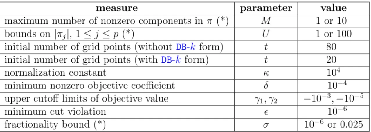
The values of various model parameters used in the computation are summarized in

Ta-ble 4.1. An asterisk (*) indicates that the parameter does not apply to all experiments.

We also present below a brief motivation for our choices.

measure parameter value

maximum number of nonzero components in π (*) M 1 or10

bounds on|πj|, 1≤j ≤p(*) U 1or 100

initial number of grid points (without DB-k form) t 80

initial number of grid points (with DB-k form) t 20

normalization constant κ 104

minimum nonzero objective coefficient δ 10−4

upper cutoff limits of objective value γ1, γ2 −10−3,−10−5

minimum cut violation 10−6

fractionality bound (*) σ 10−6 or0.025

Table 4.1: Model parameter values used in computation

(42)

cuts are essentially lift-and-project cuts1_{. Therefore, in a way to test the reliability of our}

implementation, we first set M = 1 and compare the computational results with those of

the lift-and-project closure by Bonami et al [21].

In their experimental analysis, Balas and Saxena [13] noted that the split disjunctions

they computed generally featured two interesting characteristics. Although not being in-tentionally restricted,

(i) most split disjunctions had a support of size between 10 and 20, irrespective of the size of the problem; and

(ii) most split disjunctions did not have very large coefficients, with the average coefficient size per iteration typically being less than 5.

We chose the sparsity parameter of M = 10 to reflect the lower end of that spectrum.

When attempting to limit the size of the split coefficients, we chose bounds U = 1 (i.e.,

−1≤πj ≤1, for all 1≤j ≤p) since these would be the simplest splits obtainable. When

“only” sparsity constraints were enforced, we actually set U = 100 (i.e., −100≤πj ≤100,

for all 1 ≤ j ≤ p). This allows for splits with somewhat larger coefficients, but we still

need U to be finite for practical reasons.

At each iteration, the initial parameter grid size depends on whether a DB-k form of

the constraint matrix is supplied or not. If no DB-k form is given, we set t = 80, and 80

MILP(θ)’s are processed; if a decomposition is given, then we set t = 20 for each of the k

blocks, and therefore20k MILP(θ)’s are processed in total.

For the fractionality bound σ on the set of split disjunctions, a natural value could be,

for example, the integrality tolerance10−6. In general, more cuts may be obtained by using

such a loose bound, and we thus set σ = 10−6 _{when trying to reproduce lift-and-project}

results of Bonami [21]. In all the other experiments, however, we impose a rather strict

bound σ = 0.025. This led to more gap closed per iteration on average and more gap

closed overall within our time limits. Adding a fractionality bound also helped preventing

MILP(θ)’s from yielding unviolated split disjunctions due to numerical errors.

1_{Original ideas of the lift-and-project approach dates back to the early 1970’s in the context of} dis-junctive programming, see Balas [9]. More explicit reformulation techniques for integer programs with all binary variables are proposed by Sherali and Adams [46], and by Lovász and Schrijver [43]. When lift-and-project is applied to a single variablexj, Balas et al. [11] showed that it is equivalent to considering

P(ej,0) _{(c.f. Section} _1.3_{), i.e., a disjunctive programming problem. Therefore, for general MIPs, we say}

that any inequality valid forP(ej,π0) _{for some integer variable}_x

(43)

4.2 Three experiments

4.2.1 How does our implementation compare with known results?

To check whether our implementation was reasonable, we performed two tests.

First, we tested the code on both MIPLIB 3.0 [19] and MIPLIB 2003 [5] instances, in

a configuration where it approximates2 _{a lift-and-project cut separator. We restricted the}

sparsity parameter M = 1in order to allow only one nonzero element in split disjunctions,

thus forcing our split cut separator to return lift-and-project cuts only. Since M = 1,

we upper bounded, without loss of generality, the magnitude of disjunction coefficients by

U = 1. The entire computation time for each instance is limited to one week, including

the time taken to check cut validity. At termination, we measure the final percentage of integrality gap closed (GAPnew), which is then compared with the bounds (GAPknown)

given in [21]. For each instance, we look at the percentage of gap closed divided by the

analogous results in [21], i.e., we compute

relative gap closed:= GAPnew

GAPknown.

Therefore, a 50% relative gap closed means that our result is equal to 50% of the known gap, and a 100% relative gap closed means that our result is exactly the same as the known gap. Note that, however, due to numerical tolerances, a 99% relative gap closed would usually mean the results are identical.

We do this comparison on the 57 MIPLIB 3.0 instances where the gaps in [21] are strictly

positive. Table4.2 shows the number of instances that fall within various categories based

on this ratio. In particular, on 49 (out of 57) instances we closed at least 99% relative gap, and on 54 (out of 57) instances we closed at least 90% relative gap. The distribution

of relative gaps for MIPLIB 2003 instances is similar. Appendix A.1 and A.2 contain the

details of gap closed for each of MIPLIB 3.0 and MIPLIB 2003 instances, respectively.

Note that our implementation, which involves solving a large sequence of MILP(θ)’s, is

not designed for lift-and-project cut, as the separation problem for lift-and-project cuts can

be done by solving linear programs only [21]. Therefore, it is reasonable to expect that on

some instances we could obtain a low percentage on the relative gap closed. It is somewhat

striking to observe how close our results are to the results given in [21], considering that

our approach is completely different, yet on many instances the gaps are identical within

a±0.01% tolerance.

(44)

relative gap closed # instances

≥ 99% 49

≥ 90% 54

≥ 50% 57

Table 4.2: Gap closed as a percentage of the known gap for the lift-and-project closure

(from [21])

relative gap closed # instances

>100% 8

≥ 99% 25

≥ 90% 30

≥ 50% 31

< 1% 23

Table 4.3: Gap closed as a percentage of the best known gap for the split closure

(from [13] and [29])

Second, we tested the code on the MIPLIB 3.0 instances, in a configuration where it approximates a straightforward split cut separator, i.e., without any sparsity or structure

constraints on the split disjunctions. Artificial lower and upper bounds±100 are applied

on the disjunction coefficients (U = 100), which allows for a reasonably large subset of

all disjunctions to be considered. As in our first test, we limited the entire computation

time for each instance to one week, including the time taken to check cut validity3_{. At}

termination, we measure the final percentage of integrality gap closed, which is then

com-pared with the best of the bounds given in [13] and [29]. For each instance, we look at the

percentage of gap closure divided by the best of the analogous results in [13] and [29]. We

do this comparison on the 57 instances where the best known gaps are strictly positive.

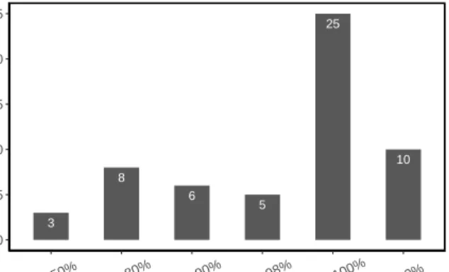
Table 4.3 shows the number of instances that fall within various categories based on this

ratio. On 8 (out of 57) instances we closed more gap than the best available result, and on 30 (out of 57) instances we closed at least 90% relative gap.

On the other hand, we closed less than 1% relative gap on 23 (out of 57) instances.

As shown in Figure 4.1 where each dot represents an individual instance, those are

gen-erally the instances that have the most integer variables. While there are many plausible explanations for our poor performance in this large set of instances, an important one is that the parameters in our code were not fine-tuned for this experiment, but rather for

(45)

0% 50% 100% 150% 200% 10 100 1000 10000 1e+05

Number of integer variables

Relativ

e gap closed

Figure 4.1: Gap closed as a percentage of the best known gap closure (from [13]

and [29]), vs. number of integer variables

the experiments considering sparsity. When changing the values of parameters such as the

number|Θ|of grid points and the fractionality boundσ, we were able to close significantly

more gap on these 23 instances.

The purpose of this experiment was to determine if our implementation was reliable,

compared to other ones. Our highly consistent lift-and-project results (M = 1)

demon-strate that the implementation was indeed reasonable. Although the results on general split cuts were not as convincing, it is sensible to expect that they would match with the best known results had we chosen a longer computation time limit and fine-tuned the parameters (this is omitted because the fine-tuning of the parameters is not the primary goal of this work). Finally, we note that the reliability of our implementation is further evidenced by the experiments in subsequent sections.

4.2.2 How does sparsity help?

In this section, we evaluate the relative strength of split cuts (i) whose split disjunctions are sparse and (ii) whose split coefficients are also small. We ran our implementation again on the MIPLIB 3.0 instances, first with the additional sparsity constraint obtained by setting

M = 10. Then, we additionally considered ±1 bounds on the disjunction coefficients

(that is, setting U = 1). As was the case earlier, a time limit of one week was set for all

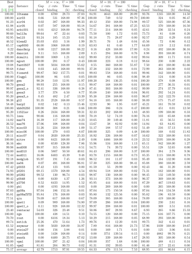
computations. Table 4.4 shows the details of our results. The first column of the table

shows the best of the gaps given in [13] and [29], followed by results obtained with arbitrary