Dissertations 2019
Efficient state estimation via inference on a probabilistic graphical
Efficient state estimation via inference on a probabilistic graphical
model
model
Luke David Myers Iowa State University
Follow this and additional works at: https://lib.dr.iastate.edu/etd Part of the Electrical and Electronics Commons
Recommended Citation Recommended Citation
Myers, Luke David, "Efficient state estimation via inference on a probabilistic graphical model" (2019). Graduate Theses and Dissertations. 17520.
https://lib.dr.iastate.edu/etd/17520
This Thesis is brought to you for free and open access by the Iowa State University Capstones, Theses and Dissertations at Iowa State University Digital Repository. It has been accepted for inclusion in Graduate Theses and Dissertations by an authorized administrator of Iowa State University Digital Repository. For more information, please contact [email protected].
by
Luke David Myers
A thesis submitted to the graduate faculty
in partial fulfillment of the requirements for the degree of MASTER OF SCIENCE
Major: Electrical Engineering (Electric Power and Energy Systems)
Program of Study Committee: Daji Qiao, Major Professor
Zhenqiang Gong Venkataramana Ajjarapu
The student author, whose presentation of the scholarship herein was approved by the program of study committee, is solely responsible for the content of this thesis. The Graduate College will ensure this thesis
is globally accessible and will not permit alterations after a degree is conferred.
Iowa State University Ames, Iowa
2019
DEDICATION
I would like to dedicate this thesis to my father, who has always supported and encouraged me both in my educational endeavors as well as in every other area of my life.
TABLE OF CONTENTS
Page
LIST OF TABLES . . . vi
LIST OF FIGURES . . . vii
ACKNOWLEDGMENTS . . . viii ABSTRACT . . . ix CHAPTER 1. INTRODUCTION . . . 1 1.1 Background . . . 1 1.2 Our Contributions . . . 2 1.3 Organization . . . 3 1.4 My Own Contributions . . . 3
CHAPTER 2. STATE ESTIMATION . . . 4
2.1 State Estimation On DC And AC Flow Models . . . 4
2.2 Existing SE Solvers . . . 6
2.3 A 3-bus Example . . . 7
2.4 Discussion . . . 9
CHAPTER 3. PROBABILISTIC GRAPHICAL MODEL . . . 10
3.1 Markov Networks, Node Potential, And Edge Potential . . . 10
3.2 Inference Via Belief Propagation . . . 11
CHAPTER 4. STATE ESTIMATION: A PGM PERSPECTIVE . . . 13
4.1 Modeling A Power Grid As A Graph . . . 14
4.2.1 Transforming DC SE To Inference Problem On A PGM . . . 15
4.2.2 Transforming AC SE To Inference Problem On A PGM . . . 17
4.2.3 Example . . . 17
4.3 Solving The PGM Problem Via Gaussian Belief Propagation . . . 19
4.3.1 Gaussian Belief Propagation . . . 19
4.3.2 Speeding Up Message-Passing In GBP . . . 20
4.3.3 Example . . . 22
4.4 Existing SE Solvers Versus Our Proposed PGM/GBP Solver . . . 22
4.5 Complexity Analysis . . . 23
CHAPTER 5. PERFORMANCE EVALUATION: PGM . . . 25
5.1 Experimental Setup . . . 25
5.2 AC SE Versus AC PGM: State Estimates . . . 25
5.3 AC SE Versus AC PGM: Running Time . . . 26
CHAPTER 6. APPLICATION: DEFENSE AGAINST FALSE DATA INJECTION ATTACKS . . . 28
6.1 State Estimation (SE) And Bad Data Detection (BDD) . . . 28
6.2 False Data Injection Attacks (FDIAs) . . . 29
6.3 Defense Against FDIAs . . . 32
6.4 AC-Based Defense . . . 32
CHAPTER 7. PERFORMANCE EVALUATION: DEFENSE AGAINST FDIA . . . 36
7.1 Experimental Setup . . . 36
7.2 Susceptibility Of DC SE To FDIA . . . 37
7.2.1 Successful Attack Ratio When Attacker Has Full Access To All Meters . . . 37
7.2.2 Meters Needed For A Successful Attack . . . 38
7.3 AC SE/PGM Defense Against FDIA . . . 38
CHAPTER 8. CONCLUSION . . . 41
APPENDIX A. MATLAB METER MEASUREMENT GENERATION . . . 45
LIST OF TABLES
Page
Table 2.1 Terms and notations used in Chapters2to4 . . . 5
Table 6.1 Terms and notations used in Chapter6 . . . 28
LIST OF FIGURES
Page
Figure 2.1 3-bus power grid example . . . 7
Figure 3.1 Sum-product rule . . . 11
Figure 3.2 Product rule . . . 12
Figure 4.1 Flowchart of existing SE solvers . . . 13
Figure 4.2 Flowchart of our proposed PGM method . . . 13
Figure 4.3 Graph representation of 3-bus power grid example and corresponding PGM graph . 14 Figure 5.1 Comparison of state estimates for AC SE and AC PGM . . . 26
Figure 5.2 Comparison of running time for AC SE and AC PGM . . . 27
Figure 7.1 Successful attack ratio versus number of compromised states . . . 38
Figure 7.2 Fraction of attacked meters versus number of compromised states . . . 39
ACKNOWLEDGMENTS
I want to express my gratitude and thanks to those who have assisted me in conducting the research for this thesis during my graduate studies. First of all, I would like to thank my Major Professor Dr. Daji Qiao for all of his guidance, motivation, and support throughout this research. I would also like to thank fellow graduate student Binghui Wang for his work in developing the probabilistic graphical model and indispensable contributions to the research behind this thesis. Additionally, I want to thank my committee members Dr. Zhenqiang Gong and Dr. Venkataramana Ajjarapu, as well as Dr. Guan, Grant Johnson, and Benjamin Blakely, for their help and oversight throughout this research. Finally, I would like to thank Argonne National Laboratory and Ames Laboratory for their financial support of this research during my time as a graduate student.
ABSTRACT
This thesis presents a unique and efficient solver to the state estimation (SE) problem for the power grid, based on probabilistic graphical models (PGMs). SE is a method of estimating the varying state values of voltage magnitude and phase at every bus within a power grid based on meter measurements. However, existing SE solvers are notorious for their computational inefficiency to calculate the matrix inverse, and hence slow convergence to produce the final state estimates. The proposed PGM-based solver estimates the state values from a different perspective. Instead of calculating the matrix inverse directly, it models the power grid as a PGM, and then assigns potentials to nodes and edges of the PGM, based on the physical constraints of the power grid. This way, the original SE problem is transformed into an equivalent proba-bilistic inference problem on the PGM, for which two efficient algorithms are proposed based on Gaussian belief propagation (GBP). The equivalence between the proposed PGM-based solver and existing SE solvers is shown in terms of state estimates, and it is experimentally demonstrated that this new method converges much faster than existing solvers.
CHAPTER 1. INTRODUCTION
1.1 Background
Power grid is a complex energy delivery system comprised of a large number of individual components and geographically dispersed communication systems. State estimation (SE) is a method of estimating the varying state values of voltage magnitude and phase at every bus of a power grid. This is done by taking a series of meter measurements of key parameters across the network and relaying those measurements to the control center. These meter measurements are then used to estimate the voltage states based upon their physical relations.
SE can be classified as DC SE and AC SE. AC SE estimates state values by solving a system of (complex) nonlinear equations (considering both real and reactive power), while DC SE utilizes a linear approximation of the nonlinear real power flow equations in AC SE to estimate the state values (while neglecting reactive
power) [1, 2]. Existing solvers to both DC SE and AC SE involve the calculation of the inverse of a
matrix. Direct matrix inverse methods (e.g., Gaussian elimination algorithm) are computationally infeasible if the scale of the power grid (and hence the size of the matrix) is large. Iterative methods, such as the Jacobi iterative method and the Gauss–Seidel iterative method, can avoid the calculation of matrix inverse. However, one major issue with the iterative methods [3] is that they may require a very large number of iterations and converge slowly or even cannot converge. To address this issue, we propose to solve SE from a different probabilistic graphical model (PGM) perspective, which converges much faster and thus is a much more efficient solution to the SE problem.
PGM [4] is a technique that offers a compact graph-based representation of joint probability distribu-tions, and exploits conditional independencies among the random variables. PGM has been widely used in many research areas such as machine learning, signal processing, computer vision, and data mining. To the best of our knowledge, we are the first ones to leverage PGM to improve the efficiency of state estimation.
The key idea of our proposed PGM solver to the SE problem is to represent a power grid as a PGM, and then transform the original SE problem into an equivalent probabilistic inference problem on the PGM. By doing so, the physical constraints and relations between components in the power grid are considered explicitly in the PGM and during the computation. Moreover, by utilizing the Gaussian belief propagation (GBP) algorithm to perform the probabilistic inference, each node in the PGM takes messages from all of its neighbor nodes at each iteration, thus progressing more toward the final estimates at each iteration. Hence, our proposed PGM solver requires much fewer iterations to converge.
Given the fast converging property of the proposed PGM solver, it has many potential applications. For example, it can be used, together with the AC flow model, as an efficient and practical defense to the well-known and well-studied false data injection attack (FDIA) [1] against a power grid.
1.2 Our Contributions
The contributions of this thesis include:
• We propose a novel framework to perform SE based on probabilistic graphical models (PGMs).
• We design two Gaussian belief propagation (GBP) algorithms to perform the probabilistic
infer-ence on our PGM.
• We prove and demonstrate the equivalence between existing SE solvers and the proposed PGM
solver in terms of state estimates.
• We demonstrate experimentally that the proposed PGM solver requires a much shorter running
time than standard SE solvers, particularly when the power grid is large.
• As an example application of the proposed PGM solver, we show that it can effectively and quickly
detect the FDIA, when used together with the AC flow model.
• All experiments are conducted with the MATPOWER simulator [5]. Codes are developed to
per-form DC SE and the proposed PGM solver, and to produce the meter measurements, for a variety of power grid models.
1.3 Organization
The rest of this thesis is organized as follows. In Chapter2, we provide a brief overview of SE on both
DC and AC flow models, existing methods to solve SE, and FDIA against DC SE. In Chapter3, we show
the background of probabilistic graphical model (PGM) and the inference algorithm. Chapter4details our
proposed PGM and designs two inference algorithms to solve SE. Chapter5evaluates our proposed method
on a series of experiments that compare PGM with standard SE. Chapter6explores the applicability of AC
PGM as a means of defense against FDIAs. Chapter7evaluates the resilience of PGM to FDIAs through
a number of experiments. Finally, the thesis is concluded in Chapter 8. Appendices A and B include
MATLAB code that was generated to perform some of the experiments.
1.4 My Own Contributions
Since I am not the sole individual responsible for the research for, work on, and composition of all the material presented in this thesis, it is necessary that I identify my own personal contributions before moving forward. I am largely responsible for most of the background research and work on standard DC
SE, AC SE, and FDIA reflected in Chapters1,2, and6. I also conducted all of the experiments detailed in
Chapters5and7(with the exception of running the PGM tests in Chapter5). The MATLAB code included
in AppendicesAandBare also contributions for which I am solely responsible. In addition to this, I am
responsible for having edited all of the material presented in this thesis.
Chapters 3–4, which detail our probabilistic graphical model and its application to the power grid for
state estimation, is almost exclusively the work of Binghui Wang, who is the only other main contributor to the content contained in this thesis. Where appropriate, I use singular personal pronouns throughout this
thesis to refer to myself as the main contributor. The use of plural pronouns outside of Chapters3–4are
used to indicate joint contribution on the part of both Binghui Wang and myself. Other contributors to the work behind this thesis are Dr. Daji Qiao and Dr. Zhenqiang Gong, who oversaw my research process and provided me with invaluable guidance and direction. It should also be noted that we have submitted a paper
for publication in IEEE Transactions on Smart Grid that includes much of the material presented in this
CHAPTER 2. STATE ESTIMATION
2.1 State Estimation On DC And AC Flow Models
State estimation (SE) is a method of estimating state variables of a power grid so that operators can
monitor them from the control center. The state variables of interest are the voltage magnitude, |u|, and
phase, θu, at every bus in the network. In order to perform SE for a given power system, a set of meter
measurements need to be taken of various components across the network and reported to the control center. These meter measurements can then be used along with topology information of the grid to estimate the
state variables. Table2.1summarizes the terms and notations used in Chapters2to4.
When performing SE, one of the generator buses in the power system is selected to be the slack or
reference bus, at which the voltage phase is defined asθu=0 radians. This leaves 2N−1 unknown states
to be estimated, whereNis the number of buses in the system. The task of SE is to estimate these 2N−1
states, given the meter measurements and the network topology of the power system. At least 2N−1 meter
measurements are required to estimate 2N−1 states.
Let m represent the number of states (m=2N−1) and n represent the number of meter
measure-ments (n>m) utilized to perform state estimation. Moreover, we denote the m state variables as x=
[x1,x2, . . . ,xm]T, n meter measurements as z= [z1,z1,· · ·,zn]T, and the meter measurement errors ase= [e1,e1,· · ·,en]T. Then, the relation betweenx,z, andeis encoded in the following system of equations:
z=h(x) +e, (2.1)
where h(x) = [h1(x1,· · ·,xm),h2(x1,· · ·,xm),· · ·,hn(x1,· · ·,xm)]T is an n-dim vector function that
estab-lishes dependencies betweenxandz. Each meter measurement erroreiis assumed to be Gaussian-distributed
Table 2.1 Terms and notations used in Chapters2to4
Symbol Definition
SE State estimation AC SE Nonlinear state estimation DC SE Linear state estimation
|u| Voltage magnitude θu Voltage phase N Number of buses m Number of states n Number of measurements x State variables z Meter measurements e Meter measurement errors J(x) Objective function
Λ Matrix of meter measurement error variances
H Jacobian matrix
˜
x Augmented state variables ˜
z Augmented meter measurements ˜
H Augmented Jacobian matrix
φv˜i(xi˜) Node potential
ψv˜i,v˜j(x˜i,x˜j) Edge potential
The goal of SE is to estimate state variables that best fit Eq. (2.1). Specifically, SE aims to minimize the following objective function:
J(x) =1 2 n
∑
i=1 z i−hi(x) σi 2 =1 2(z−h(x)) T Λ(z−h(x)), (2.2)whereΛis a diagonal matrix whose elements are reciprocals of the variances of meter measurement errors,
i.e.,Λ=diag(σ1−2,σ2−2,· · ·,σn−2). Moreover, a matrixH(x)that contains the derivative ofh(x)with respect
to each state variable xi is needed. Specifically, it is an n×mJacobian matrix with full column rank, as
follows: H(x) = ∂h1(x) ∂x1 ∂h1(x) ∂x2 · · · ∂h1(x) ∂xm ∂h2(x) ∂x1 ∂h2(x) ∂x2 · · · ∂hn(x) ∂xm · · · ∂hn(x) ∂x1 ∂hn(x) ∂x2 · · · ∂hn(x) ∂xm . (2.3)
Ifh(x)relates state variables to meter measurementslinearly, i.e.,h(x) =Hxwith a constant matrixH,
the above SE problem is called DC SE. In contrast, if h(x) relates state variables to meter measurements
nonlinearly, the above SE problem is called AC SE.
2.2 Existing SE Solvers
Existing solutions to SE are based on the fact that, at the minimum ofJ(x), the first-order optimality
conditions have to be satisfied. That is,
g(x) =∂J(x)
∂x =−H
T(x)
Λ(z−h(x)) =0. (2.4)
In DC SE, the closed-form solution to Eq. (2.4) can be derived, which is in the following form:
x= (HTΛH)−1HTΛz, (2.5)
In AC SE, sinceh(x)is a nonlinear function of state variablesx, a closed-form solution to Eq. (2.4) can-not be obtained. In practice, Newton-type methods are often used to iteratively estimate the state variables.
Specifically, the Newton method performs a Taylor series expansion ofg(x)around x(k), and neglects the
higher-order terms. That is,
g(x(k)+∆x(k)) =g(x(k)) +G(x(k))∆x(k)=0, (2.6) where G(x(k)) =∂g(x (k)) ∂x =H(x (k))TΛH(x(k)). (2.7)
Then, with an initial settingx(0), the Newton method iteratively updatesx(k)fork=1,2,· · ·,as follows:
∆x(k)=−(G(x(k)))−1g(x(k)) = H(x(k))TΛH(x(k))−1
H(x(k))TΛ(z−h(x(k))); (2.8) x(k+1)=x(k)+∆x(k). (2.9)
Finally, the iterative process is terminated when the`∞-norm of∆x(k)is less than a predefined thresholdε,
or when the process reaches a predefined maximal number of iterationsT.
2.3 A 3-bus Example
I will now use a simple 3-bus power grid model (which is taken from problem 9.1 in [6]) to illustrate
the SE process. The 3-bus model is shown in Fig. 2.1. The available information for the 3-bus model
includes the voltage magnitude at each bus (1 per unit or 1pu), the real power measurements on each of
the three transmission lines connecting the buses: z= [0.6pu,0.04pu,0.405pu]T, the standard deviation of
the meter measurements:σ= [0.02pu,0.01pu,0.002pu]T, and the susceptance on each of the transmission
lines: b12=5pu,b10=2.5pu,b20=4pu.
Figure 2.1 An example 3-bus power grid with 3 meters (M12,M10,M20) measuring the real power flow
across the transmission lines. The line susceptances areb12=5pu,b10=2.5pu, andb20=4pu,
respectively, with a 100 MVA base. Two states,|u|andθ, are present at each of the three buses.
In this example, all the voltage magnitudes are assumed to be 1pu. With Bus 0 being the slack
The unknown states to be estimated areθ1(the voltage phase at Bus 1) andθ2(the voltage phase at Bus
2). For AC SE, we use the nonlinear real power flow equations, as follows:
h1(x) =P12=b12sin(θ1−θ2) =5 sin(θ1−θ2); h2(x) =P10=b10sin(θ1−θ0) =2.5 sinθ1; h3(x) =P20=b20sin(θ0−θ2) =−4 sinθ2.
Sinceh(x)is made up of nonlinear equations, the Jacobian is a function of the unknown states:
H(x) = 5 cos(θ1−θ2) −5 cos(θ1−θ2) 2.5 cos(θ1) 0 0 −4 cos(θ2) .
For DC SE, we use the linear approximations of the above real power flow equations, as follows:
h1(x)≈5θ1−5θ2; h2(x)≈2.5θ1; h3(x)≈ −4θ2.
As a result, the Jacobian becomes a constant matrix:
H(x) =H= 5 −5 2.5 0 0 −4 .
With Λ=diag(0.02−2,0.01−2,0.002−2), we have everything needed to obtain the state estimates, ˆx.
Performing AC SE with Eq. (2.8), we obtain the estimates ofθ1 andθ2 as 0.0174 and−0.1014 radians,
respectively. Performing DC SE with Eq. (2.5), we obtain the estimates ofθ1andθ2as 0.0174 and−0.1013
radians, respectively. Since this example network is a very simple 3-bus system, the results of AC SE and DC SE are very close to each other.
2.4 Discussion
Note that both Eq. (2.5) and Eq. (2.8) involve the calculation of the inverse of a matrix. As noted previously, direct matrix inverse methods are computationally infeasible if the matrix size is large, while iterative methods may require a very large number of iterations and converge slowly or even cannot converge. To address this issue, we propose a novel method to solve the SE problem from a different probabilistic graphical model (PGM) perspective, which we will show converges much faster than existing solvers.
CHAPTER 3. PROBABILISTIC GRAPHICAL MODEL
Probabilistic graphical model (PGM) [4] combines probability theory and graph theory. It offers a com-pact graph-based representation of joint probability distributions, and exploits conditional independencies among the random variables. Conditional independence can alleviate the computational burden. PGM has
been widely used in various research areas such as computer vision [7, 8], speech processing [9],
time-series and sequential data modeling [10], cognitive science [11], bioinformatics [12], signal processing [13], communications and error-correcting coding theory [14], and in the area of artificial intelligence in general. The framework of PGM could provide general techniques for inference (e.g., sum-product
message-passing algorithm, also known asbelief propagation) [15] and learning [4]. Two popular representations of
graphical models areMarkov networksbased on undirected graphs (also known as Markov random fields),
andBayesian networksbased on directed graphs (also known as belief networks). In this work, we mainly focus on Markov networks because the graphical representation of a power grid is undirected.
3.1 Markov Networks, Node Potential, And Edge Potential
Markov networks are represented by undirected graphs. Given an undirected graph ˜G= (V˜,E˜), where
˜
V is a set of nodes and ˜Eis a set of edges. Each node ˜vi∈V˜ is associated with a random variable ˜xi. Markov
networks specify anode potentialφv˜i(x˜i)(also known as “evidence”) for each node ˜vi, and specify anedge potentialψv˜i,v˜j(x˜i,x˜j) (also known as “compatibility functions”) for each edge(v˜i,v˜j)∈E˜. Then, Markov networks define a joint probability distribution over all random variables as follows:
p(x˜) =p(x1,· · ·,x|V˜|) = 1 Z
∏
˜ vi∈V˜ φv˜i(x˜i)∏
(v˜i,v˜j)∈E˜ ψv˜i,˜vj(x˜i,x˜j), (3.1)whereZ=∑x˜i∏v˜i∈V˜φv˜i(x˜i)∏(v˜i,v˜j)∈E˜ψv˜i,v˜j(x˜i,x˜j)is called thepartition function, which is used to normalize the probabilities.
Nevertheless, performing inference for each variable, i.e., calculating the marginal distribution of each variable, involves a summation of exponential terms for discrete variables, or an integration for continuous variables. This renders the direct computation intractable for a large number of variables. Fortunately, the underlying graph structure, and thereby the introduced factorization of the joint probability, can be exploited via belief propagation [15].
3.2 Inference Via Belief Propagation
Belief propagation (BP), also called sum-product, is a message-passing algorithm to perform inference on graphical models. BP is originally derived for exact inference in trees [15], and then generalized to a general graph even with loops. Specifically, BP functions by passing real-valued messages across edges in
the graph and is comprised of two computational rules:sum-productrule andproductrule.
Sum-product rule: Messagesmv˜i→v˜j(x˜j)are sent on each edge(v˜i,v˜j)∈E˜ from ˜vito ˜vj. If ˜xj is a discrete random variable, the messages are updated as follows:
mv˜i→v˜j(x˜j) =
∑
˜ xi ψv˜i,v˜j(x˜i,x˜j)φv˜i(x˜i)∏
vk∈N(v˜i)\v˜j mvk→v˜i(x˜i), (3.2)whereN(v˜i) denotes the neighbor nodes of ˜vi, andN(v˜i)\v˜j means node ˜vj is excluded from the neighbor
nodes. If ˜xj is a continuous random variable, the messages are updated as follows:
mv˜i→v˜j(x˜j) = Z ˜ xi ψv˜i,v˜j(x˜i,x˜j)φv˜i(x˜i)
∏
vk∈N(v˜i)\v˜j mvk→v˜i(x˜i)dxi. (3.3)Fig.3.1visualizes the sum-product rule.
𝑣" 𝑣# 𝑣$ 𝑣% 𝒎𝒗𝒊→𝒗𝒋(𝒙𝒋) 𝑣. 𝛟01(𝑥") 𝞿01,05(𝑥", 𝑥.) … 𝒎𝒗𝒕→𝒗𝒊(𝒙𝒊) 𝒎𝒗𝒔→𝒗𝒊(𝒙𝒊) 𝒎𝒗𝒌→𝒗𝒊(𝒙𝒊)
Product rule: If the Markov network does not have a loop, the sum-product algorithm is exact [15], meaning that, if we use the sum-product algorithm, the marginals (also known asbeliefs)p(x˜i)obtained via
the following product rule are guaranteed to converge to the true marginals:
p(x˜i) =φ˜vi(x˜i)
∏
k∈N(v˜i)
mvk→v˜i(x˜i). (3.4)
Fig.3.2visualizes the product rule.
𝑣" 𝑣# 𝑣$ 𝑣% 𝒎𝒗𝒊→𝒗𝒋(𝒙𝒋) 𝑣. 𝛟01(𝑥") … 𝒎𝒗𝒕→𝒗𝒊(𝒙𝒊) 𝒎𝒗𝒔→𝒗𝒊(𝒙𝒊) 𝒎𝒗𝒌→𝒗𝒊(𝒙𝒊)
CHAPTER 4. STATE ESTIMATION: A PGM PERSPECTIVE
In this chapter, we describe our proposed approach to perform SE from a unique perspective, based on
PGMs. Comparing with existing SE solvers (shown in Fig.4.1), our approach consists of the following three
steps (shown in Fig.4.2).
Iterative Methods (e.g., Jacobi) h(x) z Ʌ Estimated value of x
Figure 4.1 Flowchart of existing SE solvers
Graph Construction SE to PGM Transformation Solving PGM via GBP Graph PGM h(x) z Ʌ Marginal distribution of x
Figure 4.2 Flowchart of our proposed PGM method
First, we model the power grid as an undirected graph (Section 4.1). Then, we contruct a PGM and
assign potentials to nodes and edges of the PGM, based on the physical constraints of the power grid, which, in turn, transforms the original state estimation problem into an equivalent inference problem on the
PGM (Section4.2). Finally, we apply Gaussian Belief Propagation (GBP) and design two GBP algorithms
4.1 Modeling A Power Grid As A Graph
We represent the power grid as an undirected graph G= (V,E). Each nodevi∈V represents a bus.
Each edge inE represents a power transmission line between two buses. The weight of each edge is the
impedance of the corresponding power transmission line. For each nodevi∈V, a nodevj(6=vi) is a neighbor
ofviif and only if there is an edge between them. The power grid state at a node is determined by (1) the
states of its neighbors, and (2) the impedance of the transmission lines between the node and its neighbors. Therefore, we can constrain each node in the power grid graph with local equations, which describe the relation between its state and its neighbors’ states. Subsequently, we can use a set of local equations to represent the constraints for the entire power grid, which are given in Eq. (2.1).
Throughout this section, we will use the same example 3-bus power system introduced in Section 2.3
and shown in Fig. 2.1, to illustrate our proposed PGM method, step by step. In the first step, this 3-bus
power system is represented by the graph in Fig.4.3a.
(a) (b)
Figure 4.3 (a) Graph representation of the example 3-bus power system. (b) The corresponding PGM
graph.
4.2 Transforming SE To PGM Problem
The second step of our approach is to transform SE to an inference problem on a PGM. Next, we first describe how to do it for DC SE, and then we generalize it to AC SE.
4.2.1 Transforming DC SE To Inference Problem On A PGM
The goal of DC SE is to solve Eq. (2.5) to produce an estimation of state variablesx. When leveraging
PGM for probabilistic inference, we requireHto be a square matrix. However,Husually is not square in
power grids. To address this issue, we adopt the following two steps:
• Step I: We transform Eq. (2.5) to a more concise form. Specifically, we denote ˆH=Λ1/2H and ˆ
z=Λ1/2z, whereΛ1/2=diag(σ1−1,σ2−1,· · ·,σn−1). Then, Eq. (2.5) becomes:
x= HˆTHˆ−1ˆ
HTzˆ. (4.1)
• Step II: We construct an augmented(m+n)×(m+n)matrix ˜Hfor ˆHas:
˜ H= Im×m HˆT ˆ H −λIn×n , (4.2)
whereIm×mandIn×n are anm×midentity matrix and an n×nidentity matrix, respectively. λ is a
small constant. Similarly, we define an augmented(m+n)-dim vector of state variables ˜x= [x;y],
wherey is an n-dim auxiliary variable vector, and an augmented(m+n)-dim measurement vector
˜
z= [0m; ˆz], where0mis anm-dim zero vector.
Then, we have the following theorem.
Theorem 1. Asλ →0, the first m elements of the solutionx˜ to˜z=H˜x˜ are equivalent to the solutionxto
Eq. (2.5) - the original SE problem.
Proof. We split ˜z=H˜x˜ into the following two equations:
0m=x+HˆTy; (4.3)
ˆ
z=Hxˆ −λy. (4.4)
Then, by combining Eqs. (4.3) and (4.4), we have:
x= HˆTHˆ+λIm×m
−1ˆ
which is the first melements of ˜x. When λ →0, we then have Eq. (4.1), which is exactly the solution to Eq. (2.5).
Given Theorem1, we can translate the original SE problem, whose goal is to solve ˜z=H˜x˜
determinis-tically, to an equivalent probabilistic inference problem on a PGM. To be specific, we first convert ˜z=H˜x˜ to an optimization problem as follows:
˜ H˜x=z˜⇐⇒H˜˜x−z˜=0 (4.6) ⇐⇒min ˜ x 1 2x˜ TH˜˜x−z˜Tx˜ (4.7) ⇐⇒max ˜ x − 1 2x˜H˜˜x+z˜ Tx˜ , (4.8)
where the equivalence between Eq. (4.7) and Eq. (4.6) is obtained by setting the derivative of the term in
Eq. (4.7) with respect to ˜x to be zero. Then, we can obtain the solution to Eq. (2.5) via maximizing the
following joint Gaussian probability density function (pdf):
p(x˜) =exp −1 2x˜
TH˜˜x+z˜Tx˜
. (4.9)
We now can use a Markov network to characterize the joint Guassian pdf. Specifically, we begin by constructing an undirected graph ˜G= (V˜,E˜), where ˜V is a set of nodes in one-to-one correspondence with
the augmented state variables ˜x= [x;y], and ˜E is a set of undirected edges determined by the non-zero
entries of the square matrix ˜H. Then, we factorize the joint Gaussian pdf into the following form:
p(x˜) = 1 Z
∏
˜ vi∈V˜ φv˜i(x˜i)∏
(v˜i,˜vj)∈E˜ ψv˜i,v˜j(x˜i,x˜j), (4.10) where Z=∑
˜ xi∏
˜ vi∈V˜ φv˜i(xi˜)∏
(v˜i,˜vj)∈E˜ ψv˜i,v˜j(xi˜,xj˜). (4.11)φv˜i andψv˜i,v˜j are the node potential and edge potential associated with the undirected graph ˜G, which are defined as:
• node potential:φ˜vi(x˜i) =exp −
1 2H˜iix˜ 2 i +z˜ix˜i ;
• edge potential:ψv˜i,v˜j(x˜i,x˜j) =exp −
1 2x˜iH˜i jx˜j
. With the above analysis, we have the following theorem.
Theorem 2. The solutionx˜ to˜z=H˜x˜ is equal to the inference of the vector of marginal meansµ over the
graphG with the associated joint Gaussian pdf p˜ (x˜)∼N(µ,H˜−1).
The proof of Theorem2is provided in [3]. Now, with Theorem1and Theorem2, we have completed
the transformation from the original DC SE problem to the problem of probabilistic inference on a PGM.
4.2.2 Transforming AC SE To Inference Problem On A PGM
The goal of AC SE is to solve Eq. (2.4) to produce an estimation of state variablesx. However, since
h(x)is a nonlinear function ofx, we cannot obtain an analytic solution forh(x)directly, unlike we have done for DC SE. Therefore, in practice, Newton-type methods are often applied to iteratively estimate the state variables. At each iterationk, we need to calculate Eq. (2.8) to update∆x(k). For the ease of description, we rewrite Eq. (2.8) by omitting the iteration index, as follows:
∆x= HTΛH−1HTΛ(z−h(x)). (4.12)
Comparing Eq. (4.12) with Eq. (2.5), we observe that the only difference is, Eq. (4.12) uses the termz−h(x),
while Eq. (2.5) uses the termz. Therefore, we can transform the original AC SE problem to the problem of
probabilistic inference on a PGM, by simply denoting ˆz=Λ1/2(z−h(x))and then following the same steps
as in Section4.2.1for DC SE.
4.2.3 Example
Now, we continue with the 3-bus example to illustrate how to construct a PGM. In this example, since
m=2 andn=3, we introduce three auxiliary state variables: y1 for transmission line between Bus 1 and
Bus 2,y2 for transmission line between Bus 1 and Bus 0, andy3for transmission line between Bus 2 and
Bus 0, as shown in Fig.4.3a. As a result, the augmented state variables are:
˜
the augmented meter measurements are: ˜ z= [02;Λ1/2zˆ] = [0; 0; 30; 4; 202.5], (4.14) and ˜ H= I2×2 HˆT ˆ H −λI3×3 = 1 0 250 250 0 0 1 −250 0 −2000 250 −250 −λ 0 0 250 0 0 −λ 0 0 −2000 0 0 −λ . (4.15)
Each auxiliary state variable is represented as an additional node in the PGM, as shown in Fig.4.3b. Since
y1connects to and depends onθ1andθ2, node ˜v3(fory1) is connected to both ˜v1(forθ1) and ˜v2(forθ2) in
the PGM. Similarly, we connect ˜v4 (fory2) with ˜v1(forθ1), and connect ˜v5(fory3) with ˜v2(forθ2). Since
Bus 0 is the slack bus, it does not have a corresponding node in the PGM. The node potential of node ˜v1in the PGM is defined as:
φv˜1(x˜1) =exp −1 2H˜1,1x˜ 2 1+z˜1x˜1 =exp −1 2θ 2 1 . (4.16)
Similarly, we can obtain the node potentials of other nodes:
φv˜2(x˜2) =exp − 1 2θ 2 2), (4.17) φv˜3(x˜3) =exp λ 2y 2 1+30y1), (4.18) φv˜4(x˜4) =exp λ 2y 2 2+4y2), (4.19) φv˜5(x˜5) =exp λ 2y 2 3+202.5y3). (4.20)
The edge potential of edge(v˜1,v˜3)is defined as: ψv˜1,v˜3(x˜1,x˜3) =exp −1 2θ1y150h11 =exp(−125θ1y1). (4.21)
Similarly, we can obtain the edge potentials of other edges:
ψv˜1,v˜4(x˜1,x˜4) =exp −125θ1y2), (4.22)
ψv˜2,v˜3(x˜2,x˜3) =exp 125θ2y1), (4.23)
ψv˜2,v˜5(x˜2,x˜5) =exp 1000θ2y3). (4.24)
4.3 Solving The PGM Problem Via Gaussian Belief Propagation
The third step is to solve the probabilistic inference problem on the constructed PGM via belief propa-gation.
4.3.1 Gaussian Belief Propagation
As nodes in our PGM are characterized by Gaussian random variables, the associated belief propagation
algorithm is also called Gaussian belief propagation (GBP) [3,16]. As we have discussed in Section3.2, for
the graph ˜Gcomposed of node potentialsφv˜i(x˜i)and edge potentialsψ˜vi,v˜j(x˜i,x˜j), we have thesum-product rule andproductrule. With these two rules and the property that the product of Gaussian distributions is still a Gaussian distribution, we have the exact form for each passing message as follows [16]:
mv˜i→v˜j(x˜j) =N (µi j,P −1
where Pi\j=Pii+
∑
˜ vk∈N(v˜i)\v˜j Pki; (4.26) µi\j=Pi−\1j(Piiµii+∑
˜ vk∈N(v˜i)\v˜j Pkiµki; (4.27) Pi j=−H˜i j2Pi−\1j; (4.28) µi j=−Pi j−1H˜i jµi\j. (4.29)After several iterations of message passing, i.e., calculatingPi j andµi j until they converge with respect to
a smallε, we obtain the marginals of ˜xi’s which are Gaussian random variablesN(µi,Pi−1)with precision
and mean as follows:
Pi−1= (Pii+
∑
˜ vk∈N(v˜i) Pki)−1; (4.30) µi=Pi−1(Piiµii+∑
˜ vk∈N(v˜i) Pkiµki). (4.31)Finally, we obtain the solution to Eq. (2.5) as follows:
x=x˜[1 :m] = [µ1;µ2;· · ·;µm]. (4.32)
4.3.2 Speeding Up Message-Passing In GBP
Recently, it has been showed in [17, 18] that, when calculating the messagemv˜i→v˜j(x˜j) from node ˜vi to ˜vj, including the message mv˜j→v˜i(x˜i) from node ˜vj to ˜vi can speed up the computation as the passing
messages can be computed in parallel, while not sacrificing the performance. In doing so, we have: ˆ Pi=Pii+
∑
˜ vk∈N(v˜i) Pki; (4.33) ˆ µi=Pˆi−1(Piiµii+∑
˜ vk∈N(v˜i) Pkiµki); (4.34) Pi j=−H˜i j2Pˆ −1 i ; (4.35) µi j=−Pi j−1H˜i jµˆi. (4.36)Then, we have the marginal Gaussian pdfN (µi,Pi−1)for each ˜xi with precision and mean as follows: Pi−1=Pˆi−1; (4.37)
µi=Pi−1µˆi. (4.38)
The detailed implementations of our PGM/GBP solver for DC SE and AC SE are shown in Algorithm1and
Algorithm2, respectively.
Algorithm 1GBP DC (PGM/GBP solver for DC SE)
Input: G= (V,E),H,z,Λ,λ,ε, andT. Output: x˜[1 :m].
Initializet=0 andx(t)withxi(t)∼N(0,1).
InitializePii(t)=Hii˜ ,µii(t)=zi˜/Hii˜ ;Pki(t)=0,µki(t)=0,∀k6=i. InitializePi j(t+1)=∞,µi j(t+1)=∞, for(i,j)∈E.˜
InitializePi j(t+1)=0,µi j(t+1)=0, for(i,j)∈/E.˜ Construct matrix ˆH=Λ1/2Hand ˆz=Λ1/2z. Construct augmented matrix ˜H=
Im×m,HˆT; ˆH,−λIn×n. Construct augmented graph ˜G= (V˜,E˜).
while kP(t+1)−P(t)k∞≥εandkµ(t+1)−µ(t)k∞≥εandt<T do
UpdatePˆ(t+1) i =P (t) ii +∑v˜k∈N(v˜i)P (t) ki ,∀i∈V˜; Updateµˆi(t+1)= (Pˆi(t+1))−1(P(t) ii µ (t) ii +∑v˜k∈N(v˜i)P (t) ki µ (t) ki ),∀i∈V˜; UpdatePi j(t+1)=−H˜−2 i j /Pˆ (t+1) i ,∀(i,j)∈E˜; Updateµi j(t+1)=−(Pi j(t+1))−1H˜i jµˆi(t+1),∀(i,j)∈E˜; t=t+1. end while return x˜i=µ (t) i =µˆ (t) i /Pˆ (t) i ,∀i.
Algorithm 2GBP AC (PGM/GBP solver for AC SE)
Input: G= (V,E),z,Λ,λ,ε, andT. Output: x˜[1 :m].
Initializet=0 andx(t)withxi(t)∼N(0,1). Initializex(t)withx(t) i =∞. Computeh(x(t))andH(x(t)). Computez(t)=z−h(x(t)). whilekx(t+1)−x(t)k∞≥εandt<T do Compute∆x(t)=GBP DC(G,H(x(t)),z(t),Λ,λ,ε,T) Updatex(t+1)=x(t)+∆x(t). Updateh(x(t+1))andH(x(t+1)). Updatez(t+1)=z−h(x(t+1)). t=t+1. end while return x˜=x(t). 4.3.3 Example
We continue with the 3-bus example. Given the node potentials and edge potentials defined in Sec-tion 4.2.3, we can define the joint Gaussian pdf in Eq. (4.10) and use GBP to infer the marginal mean
for each ˜xi. For instance, for DC SE, by running Algorithm1 withλ =1e−5 andε =1e−5, our GBP
terminates in three iterations. The estimated mean values in the three iterations are:
µ(1)= [0.0564,−0.3291,0.4923,−0.4930,−0.0621], (4.39)
µ(2)= [0.0174,−0.1013,0.6444,−0.6441,−0.0803], (4.40) µ(3)= [0.0174,−0.1013,0.6437,−0.6434,−0.0799]. (4.41)
By selecting the first two elements ofµ(3), our PGM method yields the same results as those estimated by
existing SE solvers (i.e.,θ1=0.0174,θ2=−0.1013, as shown in Section2.3).
4.4 Existing SE Solvers Versus Our Proposed PGM/GBP Solver
Existing SE solvers either directly calculate the matrix inverse (e.g., using the Gaussian elimination al-gorithm) to obtain a closed-form solution, or leverage iterative methods (such as the Jacobi iterative method and the Gauss-Seidel iterative method) to accelerate the calculation. It has been proved in [3,17,18] that the GBP solver for a system of linear equations is identical to the Gaussian elimination algorithm, and the GBP
solver incorporating two-way message passing (i.e., speedup) is identical to the Jacobi iterative method. In
Chapter5, we will use experimental results to demonstrate the equivalence between our proposed PGM/GBP
solver and existing SE solvers in terms of state estimation results.
4.5 Complexity Analysis
Our proposed PGM/GBP solver and existing SE solvers all involve the calculation of matrix inverse: Eq. (2.5) for the DC case or Eq. (4.12) for the AC case. Without loss of generality, we only focus on the computational complexity of solving Eq. (2.5) for the DC case. Similar trends can be observed for solving Eq. (4.12) for the AC case.
As shown in Algorithm1, our method solves Eq. (2.5) in an iterative process. At each iteration, it first
calculates each ˆPiand ˆµi, with each traversing all nodes and all edges in ˜Gonce. Then, it calculates eachPi j
andµi j, which also traverse all edges in ˜Gonce. Thus, the computational complexity of our method at each
iteration is 4|E˜|+2|V˜|. From Eq. (4.2), we know that|E˜|=2|E|+ (m+n),|V˜|=m+n, and|E|>(m+n).
Therefore, the dominating computational complexity of our method at each iteration is O(|E|). WithT1
iterations to reach the stop conditions, our PGM/GBP solver has a dominating computational complexity of O(T1· |E|).
Existing SE methods solve the matrix inverse in Eq. (2.5) either directly or in an iterative process. Direct matrix inverse methods, such as the Gaussian elimination algorithm, involve matrix-matrix additions and multiplications, while iterative methods only require matrix-vector additions and multiplications. Moreover, iterative methods can exploit the matrix sparsity to further reduce the computational complexity [19]. Thus, in general, iterative methods are more efficient than direct matrix inverse methods, particularly when the matrix size is large. More specifically, direct matrix inverse methods have a computational complexity of
O(nm2+nm+m3) to obtain a closed-form solution to Eq. (2.5). Iterative methods, such as the Jacobi
iterative methods and the Gauss–Seidel iterative methods, have a computational complexity ofO(T2· |E|)
to solve Eq. (2.5), whereT2is the number of iterations to reach the same stop conditions as our PGM/GBP
The main drawback of existing SE solvers is that, under certain conditions, the iterative process
con-verges slowly or even cannot converge (i.e., diverge), which leads to a very largeT2. However, as
demon-strated empirically in [3, 18], our PGM/GBP solver converges faster and has a relatively smallT1. As a
result, it is more efficient than existing SE solvers. We will further validate this claim in Section5.3with
experimental results. The reasons for the superior efficiency performance of our proposed PGM/GBP solver may be due to the following reasons. First, by transforming the SE problem to a probabilistic inference prob-lem on a PGM, the physical constraints and relations between components in the power grid are considered explicitly in the PGM and during the computation. Second, by utilizing the GBP algorithm to perform prob-abilistic inference, each node in the PGM takes messages from all of its neighbor nodes at each iteration, thus progressing more toward the final estimates at each iteration hence a smaller number of iterations.
CHAPTER 5. PERFORMANCE EVALUATION: PGM
5.1 Experimental Setup
We have conducted a number of experiments to: (1) demonstrate the equivalence of existing SE solvers
and our proposed PGM method in terms of the resultant state estimates (Section5.2); and (2) compare their
efficiency in terms of computational time (Section5.3).
All the experiments are conducted using MATPOWER 6.0 [5], which is a power flow solver package available for MATLAB that allows one to conduct state estimation on power system test models. The
running time reported in Section 5.3 is tested on a 15-core Linux server with an Intel Core i5 2.7 GHz
processor for each core and 252.2 GB memory. We wrote our own codes for performing the proposed PGM/GBP solver for AC SE. I personally developed the code for generating the meter measurements, which
is documented in AppendixA. The parameters used throughout the experiments include:
• N: Number of buses in the network;
• σ: Meter standard deviation;
• ε: Threshold value to terminate the iterations;
• T: Maximal number of iterations;
5.2 AC SE Versus AC PGM: State Estimates
We first compare AC PGM and AC SE in terms of the estimated states. The first experiment is evaluated on the IEEE 14-bus system with varying meter standard deviations. Five trials are conducted for each level of meter standard deviation, where different meter measurements are generated according to the corresponding
standard deviation. Results are plotted in Fig.5.1a. The second experiment is evaluated on IEEE 14-bus,
30-bus, 57-bus, 118-bus, and 300-bus systems, with a fixed meter standard deviation of between 0.01 and 0.02, depending on the meter type. The configurations of these test systems can be found in their respective
respectively. Results are plotted in Fig. 5.1b. From these experiments, we observe that both methods produce almost identical state estimates, regardless of the meter accuracy or the power grid size, which demonstrates the practical equivalence between the two methods.
Note that small differences between the state estimates of the two methods have been observed in some of the trials. This is because these two methods have different structures of the iterative process and thus
may terminate at different state values. However, since the termination threshold is small (i.e.,ε=1e−4),
differences are very minimal.
0.01 0.015 0.02 0.025 0.03
: Meter standard deviation
-0.1 -0.05 0 0.05
0.1
Average difference of AC SE and PGM
(a) IEEE 14-bus
14 30 57 118 300 Number of buses (N) -0.1 -0.05 0 0.05 0.1 Difference between AC SE and PGM (b)σ=0.01 to 0.02
Figure 5.1 Comparison of state estimates for AC SE and AC PGM.
5.3 AC SE Versus AC PGM: Running Time
We compare AC PGM with AC SE in terms of running time with different bus systems and different
thresholdsε to compare their computational efficiency. The experiment is evaluated on IEEE 14-bus,
30-bus, 57-30-bus, 118-30-bus, 300-30-bus, as well as Pan European Grid Advanced Simulation and State Estimation (PEGASE) 1354-bus and Polish 3012-bus systems. The configurations of latter two systems also can be
found in MATPOWER ascase1354pegase.m[20,21] andcase3012wp.m, respectively. The maximal
num-ber of iterationsT is set to be 1000. Figs. 5.2aand5.2bdisplay the running time of the standard AC SE
a variety of real and reactive power flows are measured, and both voltage magnitude|u|and phaseθ are estimated. 14 30 57 118 300 13543012 Number of buses (N) 100 101 102 103 104 105
Running time (second)
AC SE AC PGM (a)ε=1e−4 14 30 57 118 300 13543012 Number of buses (N) 100 101 102 103 104 105
Running time (second)
AC SE AC PGM
(b)ε=1e−5
Figure 5.2 Comparison of running time for AC SE and AC PGM.
We have the following observations: First, when the number of buses (N) is smaller, AC PGM needs
slightly more running time. This is because the matrix size dominates the running time when the number of
buses is small. Recall from Section4.5that AC PGM solves a nonlinear system with matrix size(m+n)×
(m+n), while AC SE deals with a smaller nonlinear system with matrix sizem×n. Second, as the number
of buses is larger than a certain value, i.e., exceeds 300, AC PGM consumes less time than AC SE. This is
because the dominating computational complexities of both methods have the same order:O(E(H)), while
AC PGM needs far fewer iterations to converge than AC SE (see Section4.5). For instance, whenN=3012
andε=1e−5, AC PGM converges at 98 iterations and 4734 seconds, while AC SE does not even converge
within 1000 iterations or 62496 seconds.
To summarize, we have experimentally verified that our proposed PGM solver for AC SE is more com-putationally efficient, hence more practical, than existing solvers for power networks with a large number of buses.
CHAPTER 6. APPLICATION: DEFENSE AGAINST FALSE DATA INJECTION ATTACKS
With our proposed PGM method as a fast and efficient alternative to solve the SE problem, there are many practical applications for this method. In this chapter, as an example, I explain how our PGM method
may provide a practical defense against the well-known false data injection attacks (FDIAs). Table 6.1
summarizes the terms and notations used in Chapter6.
Table 6.1 Terms and notations used in Chapter6 Symbol Definition
FDIA False data injection attack BDD Bad data detection WSE orJ Weighted squared error
r Residual
SSR Sum of squared residuals
σ2 Meter measurement variance τ BDD threshold α BDD significance level za Altered measurement vector
a Attack vector xbad Corrupted state estimates
c State error injection vector
6.1 State Estimation (SE) And Bad Data Detection (BDD)
After the state variables are estimated, it is important to check whether the estimated state values are trustworthy and whether the measurements are accurate. The bad data detection (BDD) technique is used for this purpose.
BDD is performed using an objective function in the form of aweighted squared error(WSE), which is
calculated based on the estimated state values, the accuracy of the measuring meters, and the actual meter
measurements. The WSE is a weightedsum of squared residuals(SSR), where a residual is the difference
a residual ofr=z−Hx, the SSR is defined asR=||z−Hx||2, where|| · ||2is the`2-norm. The WSE can
then be determined from the SSR by taking into account the variances of the meter measurements and by assigning greater weights to the more accurate meters, as follows [22]:
J= n
∑
i=1 (zi−Hxi)2 σi2 . (6.1)Note thatJ2 follows a χ2(n−m)-distribution. Therefore, if J>τ, we say that the estimated state values
are untrustworthy with the probability of a false alarm beingα, whereτis the threshold that can be decided
using theχ2(n−m)-distribution at the significance level ofα [1].
6.2 False Data Injection Attacks (FDIAs)
In practice, for large-scale power grid systems, DC SE is a popular option to estimate state variables and correct measurement noises, because it is much more efficient than AC SE, which is computationally expensive and thus less feasible.
Unfortunately, DC SE is known to be vulnerable to false data injection attacks (FDIAs). FDIA was first reported in [1] and, since then, has been well-studied in the literature. It works as follows. The attacker alters the meter measurements in such a way that the resulting state estimates are corrupted, while the SSR and hence the WSE calculated by DC SE is the same as they would be without FDIA, thus escaping BDD.
To see this, letza be an altered measurement vector such thatza=z+a, wherezis the original meter
measurement vector andais an attack vector consisting of meter measurement errors injected by the attacker.
Further, let the corrupted state estimates bexbad =x+c, where cis the difference between the estimated
state values with and without FDIA. We designatecas the state error injection vector since it contains the
error injected by the attacker into the state estimates. Note that the SSR with FDIA is given as follows:
||za−Hxbad||=||za−H(x+c)||=||z−Hx+ (a−Hc)||. (6.2)
This tells us that FDIA can evade detection if the attacker injects an attack vectorasuch thata−Hc=0.
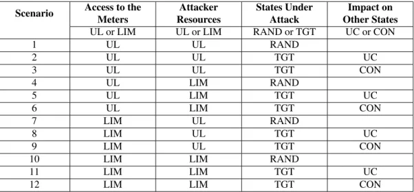
When considering such FDIA against the power grid, it is necessary and helpful to classify different kinds of attacks that a potential attacker could try to launch. [1] lists a number of different FDIA scenarios
Table 6.2 FDIA types. Attacker access to the meters: UL (unlimited) or LIM (limited). Attacker resources: UL (nlimited) or LIM (lim-ited). States under attack: RAND (random) or TGT (targeted). Impact on other states: TGT UC (targeted unconstrained) or TGT CON (targeted constrained).
Scenario Access to the Meters Attacker Resources States Under Attack Impact on Other States UL or LIM UL or LIM RAND or TGT UC or CON
1 UL UL RAND 2 UL UL TGT UC 3 UL UL TGT CON 4 UL LIM RAND 5 UL LIM TGT UC 6 UL LIM TGT CON 7 LIM UL RAND 8 LIM UL TGT UC 9 LIM UL TGT CON
10 LIM LIM RAND
11 LIM LIM TGT UC
12 LIM LIM TGT CON
(shown in Table 6.2), which can be classified according to: (1) whether an attacker has unlimited access
to all meters or only limited access to some meters in the network; (2) whether an attacker has unlimited resources with which to pollute all of the accessible meters or only limited resources with which to pollute only some of the accessible meters; and (3) whether the attacker injects random state estimates with random errors (a random FDIA) or targets specific states to inject with specific errors (a targeted FDIA).
It should be noted that a random FDIA is not the same as introducing random errors in the meter mea-surements, which can be easily detected by BDD. What is random in the case of a random FDIA is not the errors introduced into the meter measurements, but the errors injected into the state estimates. That is to say, a random FDIA takes place when the attacker introduces specific errors into specific meter measurement values such that the attack will go undetected by BDD, but does not care which states are compromised or by how much they are compromised as a result.
For targeted FDIA, on the other hand, the attacker designs the FDIA so as to inject specific state es-timate errors into specific states. In other words, there are specific states that are targeted by the attacker with the purpose of injecting specific errors into them. Targeted FDIA are distinguished into two
sub-classifications: targeted unconstrained FDIA and targeted constrained FDIA. The difference between these two sub-classifications is that for targeted unconstrained FDIA, the attacker designs the attack to introduce specific errors into the targeted states, but designs the attack such that other non-targeted states may be compromised as well. For a constrained FDIA, however, the attacker designs the attack such that only the targeted states are compromised.
I will consider one particular kind of attack in the discussion that follows- a targeted constrained attack where the attacker is assumed to have unlimited access to meters and unlimited resources. In a targeted attack, the attacker designs the FDIA so as to inject specific state estimate errors into specific states. The attack is said to be constrained in that the attacker designs the attack such that only the targeted states are compromised. I chose to focus on this FDIA scenario because: (1) the attacker is granted the advantage of being able to attack all of the meters; (2) in targeting specific states, the attacker presumably has a specific goal in mind (they want to compromise the power grid in a particular fashion); and (3) by only introducing specific false data into the targeted states, the attack may be less visible than if random errors were injected into multiple states.
To illustrate how an FDIA works, I will continue to use the same example 3-bus power system shown in Fig.2.1. Recall that I showed in Section2.3that, with DC SE, the state variables are estimated as:
x= [θ1,θ2]T= [0.0174,−0.1013]T radians. (6.3)
With the given meter measurementsz, the standard deviation of the meter measurementsσ, and the Jacobian
H, we can calculate the WSE as:
J= n
∑
i=1 (zi−Hxi)2 σi2 =0.2345. (6.4)The χ2-distribution for this example network (with 3 meter measurements and 2 unknown states) yields a
WSE threshold ofτ =6.635 for a significance level ofα =0.01. As we would expect, the WSE is well
Now, suppose the attacker intends to inject an error of 0.5 radians into state θ1. That is, the false data
injection vector isc= [0.5,0]T, and the intended corrupted state estimates are:
xbad=x+c= [0.5174,−0.1013]T. (6.5)
The attack vector needed to alter the meter measurements to generate the polluted state is:
a=Hc= 5 −5 2.5 0 0 −4 0.5 0 = 2.5 1.25 0 . (6.6)
With this attack vector added to the actual meter measurements, DC SE would yield exactly the same
WSE as above (i.e., 0.2345), thus producing the corrupted state estimatesxbad while evading BDD.
6.3 Defense Against FDIAs
Many DC SE based defenses [23,24,25,26,27,28,29,30,31,32,33,34,35] have been proposed to
deal with FDIAs. However, these defenses usually are hard to implement in practice because they often make very strong assumptions [36]. For instance, most of these defenses assume that certain meter measurements can be completed shielded from the attacker, which may not be realistic. Moreover, it has been shown in [36] that, by slightly modifying the FDIA, DC SE based defenses could be rendered ineffective.
6.4 AC-Based Defense
A more intuitive and effective way to defend against FDIAs is to simply apply AC SE to estimate the unknown states. Before illustrating this, it would be helpful to expand upon the difference between AC and
DC SE discussed in Chapter2. As was stated there, the fact that DC SE has a closed form solution makes
it significantly more efficient than the iterative methods used for AC SE. However, the closed form solution also makes DC SE more susceptible to FDIA.
Note that when performing AC SE, meter measurements are taken of both real and reactive power injections to buses and power flows across transmission lines in the network. The nonlinear equations used
to calculate the expected real (P) and reactive (Q) power flows from busito busj for AC SE are given below
in terms of the state variables (|u|andθu):
Pi j=|ui|2gi j− |ui||uj|gi jcos(θi−θj)− |ui||uj|bi jsin(θi−θj), (6.7)
Qi j=−|ui|2(bi j+bi)− |ui||uj|gi jsin(θi−θj) +|ui||uj|bi jcos(θi−θj), (6.8)
wheregi j+jbi j is the series admittance of the line and bi is the shunt susceptance at busi. For DC SE,
the series conductance (gi j) and shunt susceptance (bi) are neglected, and the voltage magnitudes at all of
the buses in the network are assumed to be 1 per-unit or 1pu. As a result, only real power flows (P) are
measured for DC SE and only the voltage phases (θu) are estimated. Assuming the voltage phases are small,
Equation (6.7) is then approximated by the following linear equation [22]:
Pi j=bi j(θi−θj). (6.9)
All of the functions used to obtain h(x) for DC SE are of this linear form. Accordingly, when the
derivative of Equation (6.9) is taken with respect to the voltage phase at every bus to obtain the Jacobian
matrixHfrom Equation2.3, the resultantHis independent of the voltage states, which is what allows for
a closed-form solution in DC SE. For AC SE, however, the Jacobian will be consistent of the derivatives of nonlinear Equations (6.7) and (6.8) with respect to the voltage states. These derivatives will themselves be nonlinear equations, making for a much more computationally complex problem, making FDIAs more difficult to implement.
To illustrate this, consider the 3-bus example. The difference here compared with DC SE is that the real power measurements are defined in terms of their actual non-linear relationships to the unknown states (as opposed to the simplified relationships used for DC). For the purposes of this example (as well as in the
voltage magnitude at every bus is 1pufor AC SE as is made for DC SE. That is to say, I am performing SE with a simplified version of AC SE in this example.
The reason I am making this assumption is so that a better comparison can be made between DC and AC SE in terms of the impact that the use of non-linear equations in AC SE makes on the ability to detect FDIA.
This example shows that by changingh(x)from a function of linear equations to non-linear equations, SE
is able to detect the FDIA that went undetected in the example in Section6.2. By implication, standard AC
SE, which does not make the assumption that the voltage magnitude of every bus is 1pu, would likewise be
able to detect FDIA.
Applying this simplified version of AC SE to the 3-bus problem with the same attack vector as in the
previous section, we will observe a significantly larger WSE (i.e.,J=13.2042 as compared withJ=0.2345
for DC SE), well exceeding the threshold for BDD (τ=6.635). As a result, the FDIA can be successfully
detected.
The reason why AC SE can successfully defend against FDIA is because it considers the underlying nonlinear dependencies between states and measurements. Thus, the Jacobian matrix in AC SE is a function of the unknown states to be estimated and changes at each iteration. This is unlike DC SE, where the Jacobian matrix is constant over all iterations. As a result, in the case of AC SE with the presence of FDIA, the altered meter measurements not only corrupt the state estimates, but also corrupt the Jacobian that is used to obtain the state estimates. This leads to a large weighted squared error, meaning that the FDIA can be detected by the BDD.
Although the AC SE-based defense is effective against FDIA, it is often considered a less practical solu-tion. This is because AC SE is computationally expensive and time-consuming due to its slow convergence or non-convergence property. Now, given that our proposed PGM solver to the AC SE problem is much more efficient than existing solvers and converges much faster, it becomes more realistic to deploy PGM-based AC SE to defend against FDIA in real power systems.
Before moving forward, it should be noted that the potential vulnerability of even nonlinear AC-based SE to FDIA has been demonstrated by Jin et al. [37], who formulated attacks against AC SE as a convex optimization problem, and solved for attack vectors via semidefinite programming. However, the proposed
attack strategy assumes that an attacker has full knowledge of the power grid system. This means that it would still be difficult for an attacker to launch an effective attack against AC SE (and by implication, AC PGM) using this approach, as full knowledge of all system meter measurements is a strong assumption. A more practical threat model would be one in which an attacker is only allowed to have partial knowledge about the system. Perhaps attacks against AC SE under more practical threat models are still possible, but to our knowledge this has yet to be demonstrated. Nevertheless, providing a means of defense against all possible threats, including those with strong assumptions, would still be ideal. That being said, any further means of defense that are developed for AC SE could theoretically be integrated into AC PGM as well, which has the added benefit of being more efficient.
CHAPTER 7. PERFORMANCE EVALUATION: DEFENSE AGAINST FDIA
7.1 Experimental Setup
I conducted a number of experiments to: (1) examine the susceptibility of DC SE to FDIA under
dif-fering conditions (Section 7.2); and (2) illustrate the immunity of AC SE/PGM to FDIAs (Section 7.3).
All of these experiments were conducted using MATPOWER 6.0 [5]. Because MATPOWER only offers an open-source code for performing AC SE, I updated the provided code to perform DC SE as well (see
AppendixB).
All of the experiments in this chapter were conducted using the IEEE 14-bus system. For the experiments
in Section7.3, I made the same assumption for AC SE/PGM as in the 3-bus example in Section6.4, namely,
that the voltage magnitudes are 1puand the same meter measurements are used for AC as DC SE/PGM.
Once again, this is done in order to offer a better comparison of the use of nonlinear versus linear equations in SE/PGM for defending against FDIA.
For convenience, I denote our GBP-based solver on PGM that solves with linear and nonlinear equations as DC PGM and AC PGM, respectively. It should be remembered for the purposes of these experiments that
the state estimate values obtained via SE and PGM are practically equivalent (see Sections4.4and5.2). For
practical considerations, all of the FDIA in these experiments wereconstrained targeted attackswith either
unlimited resourcesorlimited resources(scenarios 3 and 6 as defined in Table6.2). My reasons for using constrained targeted attackswithunlimited resourceswere explained in Section6.2. I consider FDIAs with limited resources as well to examine the susceptibility to FDIA even when the attacker is assumed to have fewer resources.
The parameters used throughout these experiments are:
• N: Number of buses in the network;
• J: Weighted squared error (WSE);
• ε: Threshold value to terminate the iterations;
• T: Maximal number of iterations;
• M: Number of states under the FDIA attack;
• K: Percentage of the meters that an attacker has resources to compromise;
• ci: State error injected into stateiunder FDIA;
By default, I set the number of states under attack toM= 2, the percentage of meters that an attacker has
resources to compromise toK= 100%, and the state error injection value toci=π/3 radians. Moreover, I
set the threshold toε = 1e−5and the maximal number of iterations toT = 1,000 for both SE and PGM. The
BDD threshold for WSE isτ =33.41, which is the threshold level for aχ2(n−m)-distribution withn=30
meters andm=13 states at a significance level ofα=0.01.
7.2 Susceptibility Of DC SE To FDIA 7.2.1 Successful Attack Ratio When Attacker Has Full Access To All Meters
In order to examine the susceptibility of DC SE to FDIA, I conducted an experiment in which the
attacker is assumed to have full access to all meters and desires to attack a specific number of states M
ranging from 1 to 13 (note that the total number of unknown voltage phase states in the IEEE 14-bus system
is 13). For eachM, I randomly generated 1,000 unique attack vectors (or less if the maximum number of
unique attack vectors for a givenMwas less than 1,000) that could be used to launch an attack against that
specific number
of states. I then determined what percentage of those attacks could be successfully launched for various amounts of attacker resources (K).
Figure7.1shows the results. We observe that asK increases, the attacker has more resources to
com-promise a greater number of meters, and thus can generate a greater number of successful attack vectors. An interesting finding is that the attacker is able to generate a successful FDIA by polluting just 20% of the meters, and can launch a successful attack against 10 states with 80% of the meters.
1 2 3 4 5 6 7 8 9 10 11 12 13 M: # States Compromised 0 0.1 0.2 0.3 0.4 0.5 0.6 0.7 0.8 0.9 1
Successful Attack Ratio
K=10% K=20% K=40% K=60% K=80% K=100%
Figure 7.1 Successful attack ratio versus number of compromised statesMand amount of resources
avail-ableK. Y-axis displays the percentage of successfully generated attack vectors with varying
amounts of resources. X-axis is the number of statesMunder attack.
7.2.2 Meters Needed For A Successful Attack
In this experiment, I investigated the percentage of total network meters an attacker needs to pollute to
launch a successful FDIA against DC SE that compromises a given number of states,M. The results, shown
in Figure7.2, confirm what we observe in Figure7.1. For instance, Figure7.2shows that between 50 and
70% of the meters would need to be polluted by an attacker in order to successfully launch an FDIA that
compromises five state values. Looking at Figure7.1, we see that an attacker won’t be able to attack five
states with only enough resources to pollute 40% or fewer of the meters, but can always launch a successful attack against five states with enough resources to pollute 80% of the meters, consistent with the results in
Figure7.2.
As we would expect, the number of meters needed to successfully launch an FDIA generally increases
as the number of states being attacked increases. This trend continues until Mis so great that all of the
available meter measurements must be altered by an attacker (11 or more for the IEEE-14 bus system).
7.3 AC SE/PGM Defense Against FDIA
To evaluate the effectiveness of AC SE/PGM based defenses against FDIAs, I simulated one particular
1 2 3 4 5 6 7 8 9 10 11 12 13 M: # States Compromised 10 20 30 40 50 60 70 80 90 100 % Meters Attacked DC
Figure 7.2 Fraction of attacked meters versus number of compromised statesM. Y-axis displays the
per-centage of meter values needed to be changed for a successful attack; X-axis displays the number of states compromised in the attack.
resources andunlimitedaccess to the meters. Once again, in atargeted attack, the attacker tries to inject
specific state estimate errors into specific states; an attack is said to be constrained in that the attacker
designs the attack in such a way that only the targeted states are corrupted [1].
In these experiments, I show the resilience of AC SE and AC PGM against FDIA. Figures7.3aand7.3b
display the weighted squared errorJfor both DC methods (DC SE and DC PGM) and AC methods (AC SE
and AC PGM) under successful FDIA against DC SE. For the experiment shown in Figure7.3a, the attack
vectors are generated for variousKandM=2. For the experiment shown in Figure7.3b, the attack vectors
are generated for variousMandK=100%. The BDD threshold is shown as the dashed line.
We observe that all attack vectors in both experiments can evade detection by DC methods, as their
generated weighted squared errors are below theχ2 threshold. However, the pollution of meter
measure-ments with these attack vectors can be easily detected by AC methods, whose weighted squared errors are much larger than the threshold. This confirms the resilience of AC SE/PGM against FDIA which are
di-rected at DC SE, as was discussed in in Section6.4. Taken in concert with the experimental conclusions of
20 40 60 80 100
K: % Meters Compromisable
102
104
106
J: Weighted Squared Error
AC DC (a) M = 2 1 2 4 8 12 M: # States Compromised 102 104 106
J: Weighted Squared Error
AC DC
(b) K = 100%
Figure 7.3 Comparison of WSE for DC SE/PGM and AC SE/PGM. In (a), we vary the percentage of
com-promisable meters (denoted as K), and in (b), we vary the number of states to attack (denoted as M).