SFB 649 Discussion Paper 2011-022
Extreme value models
in a conditional duration
intensity framework
Rodrigo Herrera*
Bernhard Schipp**
* Universidad de Talca, Chile
** Technische Universität Dresden, Germany
This research was supported by the Deutsche
Forschungsgemeinschaft through the SFB 649 "Economic Risk". http://sfb649.wiwi.hu-berlin.de
ISSN 1860-5664
SFB 649, Humboldt-Universität zu Berlin Spandauer Straße 1, D-10178 Berlin
S
FB
6
4
9
E
C
O
N
O
M
I
C
R
I
S
K
B
E
R
L
I
N
Extreme value models in a conditional duration intensity
framework
R. Herreraa,1,∗, B. Schippb
aDepartmento de Modelación y Gestión Industrial,Facultad de Ingeniería, Universidad de Talca, Camino Los
Niches Km.1- Curicó. Chile
bFaculty of Business and Economics, Technische Universität Dresden, D-01062 Dresden. Germany
Abstract
The analysis of return series from financial markets is often based on the Peaks-over-threshold (POT) model. This model assumes independent and identically distributed observations and therefore a Poisson process is used to characterize the occurrence of extreme events. However, stylized facts such as clustered extremes and serial dependence typically violate the assumption of independence. In this paper we concentrate on an alternative approach to overcome these difficulties. We consider the stochastic intensity of the point process of exceedances over a threshold in the framework of irregularly spaced data. The main idea is to model the time between exceedances through an Autoregressive Conditional Duration (ACD) model, while the marks are still being modelled by generalized Pareto distributions. The main advantage of this approach is its capability to capture the short-term behaviour of extremes without involving an arbitrary stochastic volatility model or a prefiltration of the data, which certainly impacts the estimation. We make use of the proposed model to obtain an improved estimate for the Value at Risk. The model is then applied and illustrated to transactions data from Bayer AG, a blue chip stock from the German stock market index DAX.
JEL classification: C22; C58 ; F30;
Keywords: Extreme value theory, autoregressive conditional duration, value at risk, self-exciting point process, conditional intensity.
∗Corresponding author
Email addresses:[email protected](R. Herrera),[email protected](B. Schipp)
1The financial support from the Deutsche Forschungsgemeinschaft via SFB 649 “Ökonomisches Risiko",
Humboldt-Universität zu Berlin is gratefully acknowledged. Moreover, Rodrigo Herrera thanks the Fritz Thyssen Stiftung for the financial support via a postdoctoral Fellowship.
1. Introduction
In recent years there has been a noticeable increase in the frequency and impact of extreme events and financial crises. These events range from currency crashes (Asian East 1997, Russia in 1998, Argentina in 2001), to liquidity crises (LTCM in 1998), to stock market crashes (Black Mon-day in 1987, Dot.com in 2000), to the US subprime market spillovers from 2007 through to 2009. An important aspect of these extreme events is that their impact is exacerbated by simultaneous occurrence in a multiple class of assets.
Critical questions are being asked concerning some of the quantitative methods used in risk management under the Basel II proposals. Why do extreme events occur? What measures are being taken to meet the current and certainly extreme crisis? Can researchers study former extreme events and learn how to avoid them in the future? Both theoretical and more practical oriented questions are on the actual agenda of academics, practitioners and regulators understanding of the dynamics of asset markets under stress (see Embrechts, 2009 and references therein).
The estimation of the Value at Risk (VaR) and related risk measures is a current topic of inter-est in finance, for which many approaches of varying sophistication have been derived. According to Chavez-Demoulin et al. (2005) two main approaches can be distinguished: the time series and the extreme value approach. The first emphasizes modelling the temporal features (e.g., volatility clustering and fat tails) with ARCH-type and stochastic volatility models. However, the study of extreme dependence may reveal contrasts which are obscured when we only concentrate on ex-amining the conditional second moment of a time series. Interestingly, and unlike the situation for GARCH processes (see Davis and Mikosch, 2009), there is no extremal clustering for stochastic volatility processes in either the light- or heavy-tailed cases. That is, large values of the processes do not come in clusters, which mean that the large sample behaviour of maxima is the same as that of the maxima of the associated iid sequence. On the other hand, Mikosch (2003) showed in a simulation study that for the GARCH case the expected cluster size in a set of various log-return series is smaller than for the fitted GARCH model, i.e., there is less dependence in the tails for the returns and volatilities than for the prescribed GARCH model. While these models imply some information about extreme events, still little is known about the extremes per se.
The extreme value approach makes inference on the VaR using results from Extreme Value Theory (EVT), which only focuses on the tail of the distribution (see Embrechts et al. 1997 for an introduction). The majority of the approaches on EVT for VaR estimation concern the estimation of unconditional quantiles (see for example Danielsson and De Vries, 2000, Coles, 2001 and Cotter and Dowd, 2006). An exception is the work of McNeil and Frey (2000), which addressed the conditional quantile problem and proposed a method for applying EVT to the conditional return
distribution by using a two-stage method, combining GARCH models for forecasting volatility and EVT techniques applied to the residuals from the GARCH analysis. Although this methodology works quite well in practice it has the major drawback addressed by Mikosch (2003). Thus, one should be cautious with the interpretation of the results of this method since there is no theory in the extremal clustering behaviour based on the residuals of a GARCH model.
A novel form to deal with the cluster on extremes is to use a cluster point process version of Peaks Over Theshold (POT) model introduced preliminarily in McNeil et al. (2005); Chavez-Demoulin et al. (2005) and Herrera and Schipp (2009), where the cluster of extreme data are modelled as self-exciting point processes without involving a prefiltration of data. A point process is described as self-exciting when the past evolution impacts the probability of future events. The marks contain the information that is associated with these events. The main characteristic of these models is that the intensity of occurrence of extreme events can depend on past extreme events and the size of the exceedances, allowing more realistic models.
In this paper we concentrate on a different alternative. We model the stochastic intensity of the point process of exceedances within the framework of irregularly spaced data. Contrary to the classical POT methodology, where the time of occurrence of the extreme events is modelled, the methodology proposed models the inter-exceedance times between extreme events. To this end, we use a methodology similar to an Autoregressive Conditional Duration (ACD) model (see Engle and Russell, 1998 for more reference), while the marks still being modelled by generalized Pareto distributions. Like the GARCH models, the ACD models and their alternatives (see Hautsch, 2004; Bauwens and Hautsch, 2009 and Bauwens and Hautsch, 2006) have proven to be very useful in capturing the clustering effects. For this reason, it seems natural to model the cluster behaviour of extreme observations by means of this class of processes.
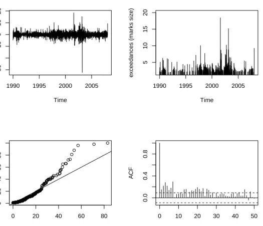
In the following we will explain our motivation in investigating extreme events in a stock market as a marked point process of exceedances. The classical POT model for iid data assumes that if the thresholduhas been chosen highly enough then the exceedances over this threshold, the extreme events, occur in time according to a homogeneous Poisson process. In addition, the size of the excess returns over the threshold, the mark sizes, are independently and identically distributed according to the generalised Pareto distribution (GPD). Figure 1.1 shows in the top panel the negative daily percentage log returns of Bayer shares between 2 January 1990 and 18 January 2008, and the times and sizes of the negative daily percentage log returns exceeding a threshold u=1,5. Observe that this contradicts the classical model assumption of no cluster at the extremes. Indeed, under a homogeneous Poisson process the inter-exceedance times should be independent exponential random variables. The lower left picture shows an exponential probability plot for the
1990 1995 2000 2005 −30 −10 0 10 20 Time Negativ e retur ns 1990 1995 2000 2005 5 10 15 20 Time e xceedances (mar ks siz e) 0 20 40 60 80 0 20 40 60 80 Theoretical Quantiles Sample quantiles 0 10 20 30 40 50 0.0 0.4 0.8 Lag A CF
Figure 1.1: Upper left panel shows Bayer daily percentage loss data from 02.01.1990 to 18.01.2008. Upper right panel displays the 732 largest losses (the exceedances). Lower left panel shows a QQ-plot of inter-exceedance times against an exponential reference distribution. Finally, the lower right panel displays the autocorrelogram for the inter-exceedance times for the exceedances.
inter-event times, these are clearly far from exponential, giving evidence against a Poisson process of exceedances. Furthermore, the autocorrelogram plot suggests clustering of the inter-exceedance times. This hypothesis is moreover reaffirmed by the Ljung-Box statistic using 10 lags. The null hypothesis of white noise is easily rejected with the Ljung-Box statistic of 217.63 well above the critical value of 18.307 at the 5% level, rejecting the Null hypothesis.
Since extreme events are inherently irregularly spaced in time and their inter-exceedance times provide strong evidence of correlation, it seems natural to study the timing of transactions as an autoregressive conditional duration model.
The main contribution of this paper from the point of view of extreme value theory is that we can capture the short-term behaviour of extremes without involving an arbitrary stochastic volatil-ity model or the prefiltration of the data, which certainly impacts the measures of risk.
Further-more, contrary to the models proposed in McNeil et al. (2005); Chavez-Demoulin et al. (2005) and Herrera and Schipp (2009), whose self-exciting functions are restricted to monotone decreasing functions, the models proposed in this paper allow hazard functions that are both monotonically decreasing and increasing. This has a logical interpretation in periods of financial turmoil, for instance, in an initial phase the VaR of a stock market initially should increase, then become close to constant and after this period decreases. To the best of our knowledge, this is the first research to take into account the incidence of the inter-exceedance times and models for irregularly spaced data in extreme value models.
The results of the application to the Bayer stock index indicate that the estimation of such models can be straightforward, derived through conditionals intensities. Different models were proposed, having in mind the simplicity of the structure of the conditional intensities. The em-pirical results show that characteristics associated with previous extreme losses as well the time between these extreme events have a significant impact on the dynamic aspects and size of future extreme events. In a VaR context the results of our backtesting procedure, which dynamically ad-justs quantiles incorporating the new information daily, allows us to statistically conclude that the models proposed are suitable for the estimation of different risk measures as the VaR, according to the restriction imposed by Basel Committee on Banking Supervision (1996, 2006).
This paper is organized as follows. In section 2 we outline relevant aspects of the classical POT model, and then in section 3 we describe the ACD-POT model theory that is central to the paper and discusse a conditional generalized Pareto distribution based approach for the exceedances. In addition, we make use of the models proposed to obtain an expression and its estimate for the VaR one day ahead predictive distribution of the returns, conditionally on the past and current data. In section 4 the models are applied to transactions data from the Bayer index. Conclusions and future works are resumed in section 5.
2. The Peaks over threshold model
In the following we will explain our motivation in investigating the consequences of modelling the inter-exceedance times in the POT framework in relation to the classical approach where only the time in which the extreme events happen are taken account.
Suppose Y1, . . . ,Yn are random variables with distribution function F which belongs to the
maximum domain of attraction ofHξ,µ,σ. ThenHξ,µ,σ is a generalized extreme value distribution
Hξ,µ,σ(y) = exp −1+ξy−σµ −1/ξ ξ 6=0, exp n −exp −y−µ σ o ξ =0,
where 1+ξy>0 ,ξ,µ ∈Randσ >0 are the shape location and scale parameter respectively.
A point process N can be viewed as a random distribution of indistinguishable points in a defined state space. For instance, the basic model for threshold exceedances in extreme value theory is based on constructing a two-dimensional point process {(ti,yi)} with state space T ×
Y = [0,1)×(u,∞). The time eventstiare the time of the i-th peak exceedance and we shall refer
to this process as the ground process, whileyi−uis the value of the exceedances for a sufficiently high thresholduand we will call this process the process of the marks. This two dimensional point process will look like as a non-homogeneous Poisson process with intensity defined for all subsets of the formA= [t1,t2)×(y,∞) wheret1 andt2 are times of occurrence of extreme events. This
representation is as follows λ(t,y) =λ(y) = 1 σ 1+ξy−µ σ −1/ξ−1 + , (2.1)
where y+ =max(y,0) and µ,σ,ξ are precisely the parameters of the generalized extreme value
distribution. Furthermore, the intensity measure of the subsetAfor anyy≥umay be expressed in the form of an one-dimensional Poisson process with intensity
τ(y) =
ˆ ∞
y
λ(s)ds=−lnHξ,µ,σ(y).
If we accept that the point process of exceedances is an one-dimensional Poisson with intensity
τ >0, then the process has independent increments, i.e., the number of events ti that occur in
disjoint time intervals are mutually independent, which implies lack of memory in the evolution of the process. In addition, the number of extreme eventstiin any interval of length (t2−t1)≥0
is Poisson distributed with mean
ˆ t2
t1 ˆ ∞
y
λ(s)dsdt =τ(y) (t2−t1).
Another important result of extreme value theory is the limiting conditional probability thatY > u+ygivenY >u τ(u+y) τ(u) = 1+ ξy σ+ξ(u−µ) −1/ξ =Gξ,β(x),
which is just the survival función of the GPD, i.e., ¯G=1−G, with scaling parameterβ =σ+ ξ(u−µ)for 0≤y<yF. HereyF is the right endpoint with valuesyF=∞ifξ>0 andyF =−β/ξ
ifξ <0.
high level of exceedances as amarked point processes(MPP). In many stochastic process models, a point process arises as the component that carries the information about the events t in time or space of objects that may themselves have a stochastic structure and stochastic dependency relations. In this paper we define a MPPN as a set of observations, occurrence times and marks
{(ti,yi)}on the spaceT ×Y, whose historyHt= ({t1,y1}, . . . ,{tt−1,yt−1})consists only of the
occurrence times and marks{t1,y1}, . . . ,{tt−1,yt−1}up to timet but not includingt. Moreover, we define a point processNg “the ground process” which refers to the stochastic process of the inter-exceedance times. This point process has a conditional density function p(t |Ht) and its corresponding survival distribution functionS(t |Ht). The conditional (finite) intensity function
(or hazard function) for the ground processNgis given by
λg(t|Ht) =
p(t|Ht) S(t|Ht)
(2.2) while the conditional intensity function for the MPPN is given by
λ(t,y|Ht) =λg(t|Ht)f(y|Ht,t) (2.3)
where f(y|Ht,t)is the density function of the marks conditional ont andHt.
Thus, the conditional intensity function with respect to the internal historyHt determines the
probability structure ofN uniquely. Furthermore, we say that a MPPN={(ti,yi)}onT ×Y has independent marks, if given the ground processNgthe marksyiare mutually independent random
variables such that its distribution depends only on the corresponding location ti. In addition,
we define a MPP as having unpredictable marks for T , if the distribution of the marks at ti is
independent of the locations and marks tj,yj for whichtj<ti. For a more formal introduction to marked point processes we refer to Daley and Vere-Jones (2003, p. 246).
According to our definition of MPP, the marks are conditionally independent of the associated ground process. Therefore, the product of mark densities simply has to be multiplied with the likelihood of the ground process. Letting N be a MPP on [t0,T)×Y for some finite positive T and let(t1,y1), . . . , tN(T),yN(T)be a realization ofN, we can obtain the log-likelihoodLof such a realization in terms of the conditional densities or intensities as
L = N(T)
∑
i=1 logpi(ti|Ht) + N(T)∑
i=1 logfi(yi|Ht,t) (2.4) = N(T)∑
i=1 logλg(ti|Ht)− ˆ T t0 λg(s|Ht)ds+ N(T)∑
i=1 logfi(yi|Ht,t)Observe that an alternative description of the non-homogeneous Poisson process (2.1) is rewrit-ten as a special case of a MPP in terms of a ground processNg with rate of the one-dimensional Poisson process of exceedances of the levelu, i.e., τ =λg(t |Ht) =−lnHξ,µ,σ(u), and a GPD function for the marks f(y|Ht,t) = β1
1+ξy−uβ −1/ξ−1 λ(t,y) =τ1 β 1+ξy−u β −1/ξ−1 . (2.5)
This is exactly the idea that we want to to explore in the next section. We will concentrate on models where the conditional intensity for the ground process will be parameterized in terms of interval between two consecutive extreme eventsxi=ti−ti−1so that the impact of a duration between successive events depends upon the number of intervening extreme events. The main area of application of these models has traditionally been in the modelling of high frequency financial data, however their structure would also seem appropriate for modelling extreme events and the tremors that follow these.
3. The Autoregresive conditional duration peaks over threshold model (ACD-POT)
As we saw in the introduction, in contrast to iid data, exceedances of a high threshold for daily financial returns do not necessarily occur according to a homogeneous Poisson process. Thus, the classical POT model is not directly applicable to financial return data.
We move away from homogeneous Poisson models for the occurrence times of exceedance of high thresholds and consider autoregressive conditional duration models for the conditional internsity of the ground processλg(t|Ht). In particular, we propose a set of models, which show
autocorrelation between inter-exceedance times, clustered extremes and non iid exceedances or marks size.
Following Engle and Russell (1998) we define a model for the conditional intensity of the ground point process of exceedances depending only on a fixed number of the most recent inter-exceedance timesxi=ti−ti−1. Letψi be the expectation of thei-th inter-exceedance time given
by
E(x|xi−1, . . . ,x1) =ψi(xi−1, . . . ,x1;θ)≡ψi, (3.1)
where θ is a parameter vector. We assume that ψi correspond to the ACD class of models. In
general the assumption is based on that for a strictly positive function with positive supportϕ(·):
R+→R+the standardized durations
εi= xi
ϕ(ψi)
are iid random variables. To derive a general expression for the conditional intensity let pbe the density function of (3.2) p xi ϕ(ψi) |Ht;θ =p xi ϕ(ψi) |θ , (3.3)
whereθ is a parameter vector. This implies that the time dependence of the duration process is
summarized by the conditional expected duration sequence. If we define again a MPP on[t0,T)×
Y for some finite positive timeT and let(t1,y1), . . . , tN(T),yN(T)be a realization ofN over the interval[0,T), one can easily show that the conditional expected intensity of the interexceedances times between extreme events, the ground process, can be expressed as a multiplicative effect between the baseline hazard function and a shift given by the expected duration
λg(t |Ht;θ) =λ0 t−tN(T) ϕ ψN(T) ! 1 ϕ ψN(T) (3.4)
Replacing further the form of the ground process defined in (2.2) by one of this type and plugging the conditional expected intensity (3.4) in (2.5) we obtain the ACD-POT model in its more general form. λ(t,y|Ht;θ) = λ0 t−tN(T) ϕ(ψN(T)) ϕ ψN(T)β 1+ξy−u β −1/ξ−1 + . (3.5)
Effectively we have combined the one-dimensional intensity in (3.4) with a generalized Pareto density. Under this model the conditional rate of crossing the thresholdx≥uat timet, given the historyHt up to that time, is
τ(t,y|Ht;θ) = ˆ ∞ y λ(t,s|Ht;θ)ds= λ0 t−tN(T) ϕ(ψN(T)) ϕ ψN(T) 1+ξy−u β −1/ξ + .
Observe that the distribution of the marks are assumed to be independent of the behavior of inter-exceedance times. Indeed, the implied distribution of the marks when an extreme event takes place is given by τ(t,u+y|Ht;θ) τ(t,u|Ht;θ) = 1+ξy β −1/ξ + =Gξ,β(y).
The estimation of the parameters of this model can be performed separately. In the first instance we can estimate the likelihood for the ground process, the conditional intensity of inter-exceedance
times, and in the second instance, the likelihood of the generalized Pareto distribution of the marks. The model proposed in (3.5) is, therefore, a model with unpredictable marks because of the fact that the distribution of the last mark att is independent of the historyHt.
Nevertheless, we also consider the case of predictable marks, i.e., the marks are conditionally generalized Pareto, given the historyHt up to the time of the mark. To this end, we parameterized
the scaling parameterβ(t,y|Ht)such that it depends on the history2. In this way, we assume that
in a period of turmoil the temporal intensity of the inter-exceedance times and the magnitude of the marks increase.
λ(t,y|Ht;θ) = λ0 t−tN(T) ϕ(ψN(T)) ϕ ψN(T) β(t,y|Ht) 1+ξ y−u β(t,y|Ht) −1/ξ−1 + . (3.6)
The features of this model immediately follow those of the first model proposed. The conditional rate of crossing the thresholdx≥uat timet, given the historyHt up to that time, is in this case
τ(t,y|Ht;θ) = ˆ ∞ y λ(t,s|Ht;θ)ds= λ0 t−tN(T) ϕ(ψN(T)) ϕ ψN(T) 1+ξ y−u β(t,y|Ht) −1/ξ + ,
while the implied distribution of the marks when an extreme observation occurs is given by
τ(t,u+y|Ht;θ) τ(t,u|Ht;θ) = 1+ξ y−u β(t,y|Ht) −1/ξ + =Gξ,β(t,y|Ht)(y).
Note that the marginal distribution of the marks will now be a conditional GPD. In the practical application, using a likelihood ratio test, we will formally test the hypothesis that the marks are unpredictable.
One main purpose of this paper is to develop a methodology to obtain an expression and its estimate for the quantile of the one day ahead predictive distribution of the returns, conditionally on the past and current data. In particular, the Value-at-risk (VaR) and Expected shortfall (ES) measures of risk. These measures have become standard measures in financial risk management due to their conceptual simplicity, computational facility and ready applicability. Following we derive these measures for the ACD-POT models.
The VaR is defined as theq-th quantile of a distributionF given by VaRtα =ytα =infy∈R:Fy
t+1|Ht(y) =α ,
2We can also parameterized the shape parameter
ξ. However, the behaviour of the estimation is severely affected.
which is solution toP(yt+1>yαt |Ht) =1−α. Observe that P yt+1>ytα |Ht = P yt+1−u>ytα−u|Ht = P yt+1−u>ytα−u|yt+1>u,Ht P(yt+1>u|Ht). (3.7)
The first term in the right hand side of equation (3.7) can be approximated via
P yt+1−u>ytα−u|yt+1>u,Ht = 1+ξ y t α−u β(t,y|Ht) −1/ξ + , while P(yt+1>u|Ht) = P(N(t,t+1) =1|Ht) = 1−exp(−λ(t,s|Ht;θ)).
Thus the VaR is defined by
VaRtα =u+β(t,y|Ht) ξ 1−α 1−exp(−λ(t,s|Ht;θ)) −ξ −1 ! . (3.8)
The last equation implies that the VaR is only defined for our models if 1−exp(−λ(t,s|Ht;θ))>
1−α. In the case of expected shortfall (ES), it is defined as the average of all losses which are
greater or equal to VaR, i.e. the average loss in the worst(1−α)% casesEStα =E[Y |Y >VaRtα].
In the models proposed the ES is given by EStα =VaR t α 1−ξ + β(t,y|Ht)−ξu 1−ξ . (3.9)
In the following sections we introduce the models that we want to utilize to parameterize the expected conditional duration functionψi, the distribution of probability of the standardized
durationsεiand the models for the scale parameterβ(t,y|Ht). 3.1. ACD models for the expected conditional duration
In this section, we consider models that allow for additive as well as multiplicative components in the conditional duration functionψ. In addition, we introduce parameterizations that allow not
The ACD model
The most popular autoregressive conditional duration model, introduced by Engle and Russell (1998), is based on a linear parameterization of the conditional mean function
ψi=w+ p
∑
j=1 ajxi−j+ q∑
j=1 bjψi−j,where w>0, a,b ≥0. In order to ensure the stationarity and existence of the unconditional expected duration we need∑pj=1aj+∑qj=1bj<1.
The logarithmic ACD (Log-ACD) model
In order to preventψibecoming negative, Bauwens and Giot (2000) introduced the
Logarith-mic ACD model in which the autoregression bears on the logarithm of the conditional expected duration. ψi=exp ( w+ p
∑
j=1 ajlogxi−j+ q∑
j=1 bjlogψi−j ) .Note that the functional form ofψi implies a multiplicative relationship between past durations
which is quite different from a linear form. The Box-Cox ACD (BCACD) model
Dufour and Engle (2000) propose the Box-Cox-ACD model as a more flexible alternative based on a Box-Cox transformation of the past innovations due to the Log-ACD model implies a relatively rigid adjustment process of the conditional mean to recent durations and thus, in general, an over adjustment of the conditional mean after very short durations.
ψi=w+ p
∑
j=1 aj δ εi−δ j−1 + q∑
j=1 bjψi−j.This specification includes the Log-ACD model for the Box-Cox parameterδ →0 and a linear
specification forδ =1.
The EXponential ACD (EXACD) model
Dufour and Engle (2000) also introduce the so called EXponential ACD Model since this model is similar to the one Nelson (1991) devised for the GARCH model. In this model the news effects are modelled with a piece-wise linear specification.
ψi=w+ p
∑
j=1 ajεi−j+δj εi−j−1 + q∑
j=1 bjψi−j.Thus, for durations shorter than the conditional mean εi−j<1
, the news impact curve has a slopeaj−δjand an interceptw+δj. Durations longer than the conditional mean εi−j>1
, also have a linear effect, but with a slopeaj+δj and interceptw−δj.
Strict stationarity of the conditional mean for the models Log-ACD, BCACD and EXACD is guaranteed by constraints on coefficientsb’s, i.e., all roots of 1−∑qj=1bjvj must lie outside the
unit circle.
3.2. Distributional assumptions for the standardized durations
The second important ingredient in the parameterization of our ACD-POT model is the dis-tributional assumption for the innovation process. In this section we explore two alternatives the Burr and the generalized gamma distribution. The major advantage of these distributions over the exponential and Weibull distribution, the most common distributions utilized in ACD models, is that these have non-monotonic hazard functions taking bathtub shaped or inverted U-shaped forms. In a bathtub shaped form the hazard rate initially decreases, during the middle phase the hazard rate is essentially constant, and in the final phase the hazard increases. Inverted U-shaped forms are the counterparts, the hazard rate initially increases, then becomes close to constant and ultimately decreases. This feature is of particular importance if we are interested in modelling risk measures such as the VaR or the expected shortfall.
Generalized Gamma distribution
Lunde (1999) as well Zhang et al. (2001) propose the use of a generalized gamma distribution to characterize the standardized durations because one can then obtain a non-monotonic hazard function and a time-varying conditional mean duration. A three parameter generalized gamma density is given by f(x|γ,k) = γx kγ−1 λkγΓ(k)exp n −x λ γo , x>0.
It includes the exponential distribution (γ =k =1), the Weibull distribution (k =1), the
half-normal (γ =1/2,k=1) and the ordinary gamma distribution (k=1). Under the restriction that λ =1 we choseϕ(ψi) =φi=ψi Γ(k)
Γ
k+1 γ
which implies a conditional density of the standardized duration given by p xi φi |Ht;θ = γ ψi xiΓ(k) xi φi kγ exp − xi φi γ
and a conditional density of the durations p(xi|Ht;θ) = γΓ k+1 γ xi xi φi kγ exp − xi φi γ ,
whereθ is once more a parameter vector. Note that ifk=1, then we get the Weibull-ACD model,
while fork=γ=1 the model reduces to an Exponential-ACD model. The hazard function implied
by the generalized gamma model may now be written as
λg(xi|Ht;θ) = γxkiγ−1 φikγΓ(k)exp n −xi φi γo I k,xi φi γ ,
where is the upper incomplete gamma integralI
k,xi φi γ =´∞ xi φi γuk−1exp(−u)du.
In addition, the shape properties of the conditional hazard function can be derived from its parameters values. If kγ <1, the hazard rate is decreasing for γ ≤1 and U-shaped for γ >1.
Conversely, if kγ >1, the hazard rate is increasing for γ ≥1, and inverted U-shaped for γ <1.
Finally, ifkγ =1, the hazard is decreasing forγ <1, constant forγ =1, and increasing forγ >1.
The conditional intensity in this case takes the form
λ(t,y|Ht;θ) = γxkiγ−1 φikγΓ(k)exp n −xi φi γo I k,xi φi γ 1 β(t,y|Ht) 1+ξ y−u β(t,y|Ht) −1/ξ−1 + .
The conditional log-likelihood function of this model on a set of observed inter-exceedance times and of marks or size of the exceedances can easily be derived of (2.4)
L = N(T)
∑
i=1 logγ+ (kγ−1)log xi φi −log(Γ(k)φi)− xi φi γ −(1+1/ξ) N(T)∑
i=1 log 1+ξ yi−u β(t,y|Ht) +Burr distribution
Another flexible alternative is the Burr distribution introduced in the context of ACD models by Grammig and Maurer (2000). The density function is defined by
f(x|λ,k,γ) = λkt
k−1
1+γ2λtkγ
−2+1
In this case we defineϕ(ψi) =φi=ψi
γ2(1+
1
k)Γ(γ−2+1)
Γ(1+1k)Γ(γ−2−1k), where 0<γ
−2<k. We choose the density
(3.3) to be Burr under the restriction thatλ =1,
p xi φi |Ht;θ = kφ 1−k i x k−1 i 1+γ2φi−kxik γ−2+1.
The conditional density ofxiis then
p(xi|Ht;θ) =
kφi−kxk−i 1
1+γ2φi−kxki
γ−2+1,
which is a Burr density with parameterλ =φi−k. The implied conditional hazard function is
λg(xi|Ht;θ) =
kφi−kxk−i 1
1+γ2φi−kxki
, (3.10)
which is non-monotonic function with respect to duration. From (3.10) can be obtained: the Weibull-ACD model if γ2→0, Exponential-ACD model if γ2→0 and k=1 and Log-Logistic
ACD forγ2=1. The conditional intensity in this case takes the form
λ(t,y|Ht;θ) = kφi−kxk−i 1 1+γ2φi−kxki 1 β(t,y|Ht) 1+ξ y−u β(t,y|Ht) −1/ξ−1 + .
The conditional log-likelihood function of this model on a set of observed inter-exceedance times and of marks or size of the exceedances can be easily obtained from (2.4), i.e.,
L =
N(T)
∑
i=1
n
logk−klogφi+ (k−1)logxi− 1+γ−2
log1+γ2φi−kxki o −(1+1/ξ) N(T)
∑
i=1 log 1+ξ yi−u β(t,y|Ht) +3.3. Models for the time varying scale parameter
In this section we consider different models to parameterize the scaling parameterβ(t,y|Ht)
such that it depends on the history. This feature implies that the marks are conditionally general-ized Pareto, given the historyHt up to the time of the mark. Under these models we assume that
in a period of turmoil the temporal intensity of the inter-exceedance times and the magnitude of the marks increase. We will specify and estimate two alternatives forms for the scaling parameter
β(t,y|Ht), the lineal
β(t,y|Ht) =ω+β1yi−1+β2ϕ(ψi)
and the exponential
β(t,y|Ht) =ω+β1yi−1+β2ϕ(ψi),
whereω,β1,β2∈R+.
The two models have in common a natural interpretation; the scaling parameter β(t,y|Ht)
depends on the last mark and the conditional mean function of the inter-exceedance times, given the information up to timet, but not includingt3.
4. Empirical application
In this section we present the main empirical results obtained by testing the models introduced in the previous sections. For the empirical test we chose the transaction data from Bayer AG as announced already in the introduction. In this study we only concentrate on the left tail, so that the daily returns are obtained asrt=−100 ln(pt/pt−1), where pt denotes the (closing) stock price at dayt. The sample period spans from 2 January 1990 to January 18, 2008, two days before January 20, when the Global stock markets suffered their biggest falls since September 11, 2001. A second sample is used for backtesting the estimation of the VaR in the Bayer AG from 20 January 2008 to January 16, 2009. In the backtest we daily update the new information that becomes available for the parameter estimates previously obtained. Thus, we dynamically adjust quantiles, which allows us to improve as accurately as possible the estimation of the risk measures.
In order to summarize adequately the large quantity of empirical results obtained, we use a classification scheme for the ACD-POT models. The first lower-case letter describes the type of
3In the first instance we take different models into account to find the best approach. Our analyses with financial
time series have suggested that by model comparisons based on the likelihood ratio statistic, these models keep the formulation easy to understand.
distributional assumption with respect to the ACD model (generalized gamma or Burr). The fol-lowing capital letters denote the type of ACD model: ACD, Log-ACD, BCACD or EXACD4. The last small letter denotes the models for the time varying scale parameter: l (lineal), e (exponential) or u (for unpredictable marks as in (3.5) or equivalently with scale parameterβ constant). For
ex-ample, a model gLog-ACDu means that we are working with a Log-ACD model for the expected conditional duration with generalized gamma distribution and unpredictable marks. In total we have 24 models.
All parametric models are estimated using quasi maximum likelihood. We adopt different models according to our scheme classification to test the different ACD models with different distributional assumptions regardless the possibility of a model with unpredictable marks (marks with iid GPD) or predictable marks (marks with GPD whose scale parameter is time-dependent). Observe that the former is equivalent to fitting separately a ACD model to the inter-exceedance times and a GPD to the excess losses over the threshold.
An important point is the choice of the threshold, which implies a balance between bias and variance. The threshold must be set high enough so that the exceedances are distributed general-ized Pareto. However, the choice of the optimal threshold is still considered an open problem and different approaches have been proposed to overcome this difficulty. In this paper we choose to work with the 10% of the maxima of the sample5.
In relation to the measures of goodness of fit we utilize the W-statistics to assess our success in modelling the temporal behaviour of the exceedances of the threshold u. This statistic states that if the GPD parameter model is correct, then the residuals are approximately independent unit exponential variables. In addition, to check that there is no further time series structure the autocorrelation function (ACF) for the residuals is also included. Similarly, we provide empirical evidence on the accuracy of actual VaR measures derived from the models. The first of them is an unconditional coverage test proposed by McNeil and Frey (2000). The idea is to test if the fraction of violations obtained for a particular risk measure, is significantly different from the theoretical one. A violation of the VaR is defined as occurring when the ex-post return is lower than the VaR. The second approach proposed by Berkowitz et al. (2009) tests for uncorrelatedness of the violations. In particular, we suggest the well-known Ljung-Box test of the violation sequence’s autocorrelation function. All these methods are resumed briefly in the Appendix.
It is quite evident that the performance of the models considered varies depending on the kind
4For a meaningful comparison of alternatives and for simplicity, we limit the dynamic structure of the ACD-POT
models to the first lag order only.
5The choice of the threshold is done with help of the the mean excess (ME) function, which is a popular tool used
0 100 200 300 400 500 0.02 0.08 0.14 Time Conditional Intensity 0 100 200 300 400 500 0.02 0.08 0.14 Time Conditional Intensity 0 100 200 300 400 500 0.02 0.08 0.14 Time Conditional Intensity 0 100 200 300 400 500 0.02 0.08 0.14 Time Conditional Intensity
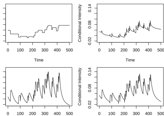
Figure 4.1: The path of the conditional intesities of an ACD-POT model under four types of distributional assump-tions: in the top panel the exponential (left) and the Weibull (right) distributions. In the bottom panel the Burr (left) and the generalized gamma (right) distributions.
of distributional assumption or the model for the time varying scale parameter, that we fitted. To gain understanding about how each class of models and distribution assumptions affect the estimations we visually compare the behaviour of the estimate conditional intensity of a small sample for the Bayer returns.
In the first instance we only concentrate on the kind of distributional assumption. In Figure 4.1 we display the path of a ACD-POT model with four types of distributional assumptions: in the top panel the exponential (left) and the Weibull (right), as especial cases of the Burr or generalized gamma distribution, and in the bottom panel the Burr (left) and the generalized gamma (right) distribution. Observe that in the case of the exponential and Weibull distributions we have a flat or monotone conditional intensity, respectively. On the other hand, both the Burr and the generalized gamma distribution show a non-monotone conditional intensity. This important feature allows to the last two distributions rapidly adapting the conditional intensity to periods of high volatility which are associated with clustering of short interexceedance times.
In relation to the type of ACD model for conditional mean duration, Figure 4.2 shows con-ditional intensities for the four models proposed under the assumption of a generalized gamma
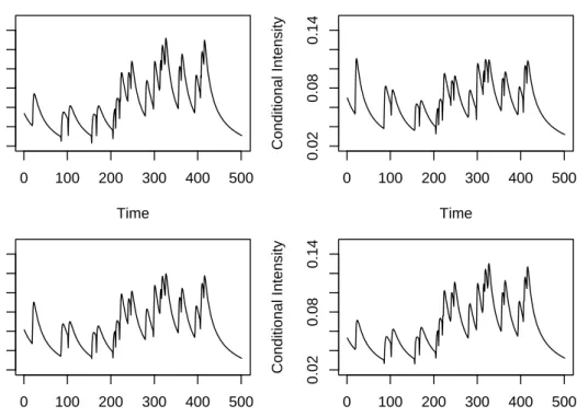
0 100 200 300 400 500 0.02 0.08 0.14 Time Conditional Intensity 0 100 200 300 400 500 0.02 0.08 0.14 Time Conditional Intensity 0 100 200 300 400 500 0.02 0.08 0.14 Time Conditional Intensity 0 100 200 300 400 500 0.02 0.08 0.14 Time Conditional Intensity
Figure 4.2: The path of the conditional intesities for the four models proposed under the assumption of a generalized gamma distribution for the innovations: the gACDu (top left), the gLog-ACDu (top right), the gEXACDu (bottom left) and the gBCACDu model (bottom right).
distribution for the innovations: the ACD (top left), the Log-ACD (top right), the EXACD (bot-tom left) and the BCACD model (bot(bot-tom right). At this stage, it is not yet possible to reach a conclusion on the appropriateness of each model. However, there are some important features of the models to keep in mind, before we make a choice. On the one hand, the Log-ACD allows for nonlinear effects of short and long durations in the conditional mean, without requiring the estimation of additional parameters in comparison to the standard ACD model. While on the other hand, the BCACD and the EXACD models offer a captivating compromise between the need of greater flexibility and the burden of higher complexity.
Empirical results
The maximum log-likelihood estimates of the ACD-POT models proposed in section 3 for the returns are displayed in Tables A.1 and A.2 in the Appendix. For the inter-exceedance times, the generalized gamma seems to be the best distribution between the two choices. The results on ACD models for the expected conditional duration lead to markedly fovour the Log-ACD specifications, followed by the ACD one. Finally, the models with time varying scale parameters lead to a better fit. Indeed, the results suggest that the models with predictable marks react more quickly to
in-creasing and dein-creasing cluster of extremes, which means that the size of the exceedances has an effect on the probability of further exceedances in the near future.
According to the AIC of the models proposed, the best fitted model for the Bayer index is a ACD model with generalized gamma distribution and lineal form for the scale parameter (gACDl) with AIC of 4067.59. We observe further that k=53.767 (36.539), γ =0.121 (0.041), which
implies thatkγ >1 andγ <1 so that the hazard rate is inverted U-shaped. This should not come
as a surprise if one is aware of the intimate relationship between durations and cluster of extremes. Furthermore, this is the sort of hazard function that earlier authors have found to be realistic in modeling the dynamics of "price durations" in stock markets (see for instance Zhang et al., 2001 and Grammig and Maurer, 2000). In relation to the results of estimation of the conditional GPD model to the excedances we obtainedξ=0.503 (0.100),ω= 0.094 (0.044),β1=5.7e-07 (0.001) and
β2= 4.492 (0.826).This result indicates that the lineal form to parameterize the scaling parameter
β(t,y|Ht), such that it depends on the history, was a good choice. Interestingly, the size of the
last exceedance is not as important as the expectation of the i-th inter-exceedance time.
Although the model of choice identified by the AIC may be seen as the best among the existing models because it shows the best global fit, this does not mean that no better model is possible for backtesting. So, we usually check whether the major features of the given data can be reproduced by the estimated models, for instance, the cluster of extreme events. If this important feature is not reproduced, we must consider further models whose AIC values can be compared with those of the previous best model. To this end, we include two other models to have a comparison of different alternatives in the backtest. The second best alternative is a Log-ACD and the third is a BCACD, both with generalized gamma distribution and lineal form for the scale parameter. We concentrate on these three alternatives and test the reliability of these models by investigating the conditional GPD assumption of the marks in the models fitted, the quality of the times component of our model and the performance in-sample of the estimated VaRs.
The results on the goodness of fit in sample are displayed in Figure A.1. More general test on miss specification in an ACD model were proposed by Meitz and Teräsvirta (2006). Here, we first assess the conditional GPD assumption of the marks in the models fitted. To this end, we provide the W-statistic explained in details in the Appendix. This statistic forms an iid se-quence of exponential random variables with mean one if the marks are GPD. According to the QQ-plots displayed in Figure A.1, we do not observe a substantial deviation from an exponential distribution. In addition, to check that there is no further time series structure, the autocorrelation function (ACF) for the residuals (middle panel) is also included. The autocorrelations is negligible at nearly all lags. Finally, to appraise the quality of the times component of our model, we employ
the residual analysis method for point processes resumed briefly in the Appendix. This is based on the change of time scale using the estimated conditional intensity. We investigated whether the transformed time-scale version of the data constitutes a homogeneous Poisson process. The resid-ual analysis for the three models indicates that the ACD-POT models in their three alternatives in the changed time scale seems to be acceptable. Hence, for the returns the ACD-POT specification seems to be appropriate.
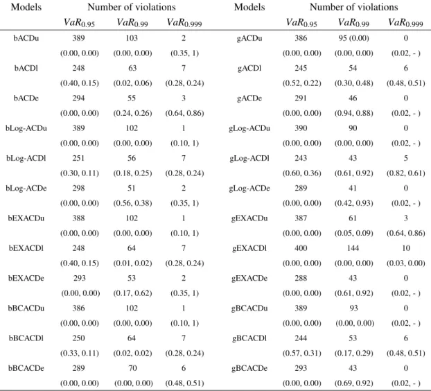
In relation to the performance in-sample of the estimates VaRs, Tables A.3 displays the results for the unconditional coverage test and the Ljung-Box test, for all the models for three different VaR levels (0.05, 0.01, and 0.001). For each model proposed in the last section we give the number of violations or failures in the VaR, the unconditional coverage test and the Ljung-Box test (the last two in brackets). In the case of these three models fitted the conditional VaR is correctly estimated for all the confidence levels6.
Backtesting the models
Backtesting provides invaluable feedback about the accuracy of the models proposed to risk managers. The performance of VaR w.r.t backtesting has been carried out with the daily returns for one year, i.e., from January 20,2008 to January 16, 2009. The backtest method consists on comparing the estimated conditional VaR for one day time horizont, given knowledge of returns up to and includingt for three different confidence levels (0.95, 0.99, and 0.999). For each day in the back test we reestimate the models, something that immediately reveals possible stability problems of a model. Then, we reestimated the risk measures for each return series according to the formula (3.8).
Table A.4 reports the results on the VaR backtesting exercise for all confidence levels, while the VaR violations for the 0.99 confidence level under the gLog-ACDl, gACDl and gBCACDl models are shown in Figure A.2. The performances for the models are similar for the results on VaR forecasting, although we observe some differences. For instance, the gLog-ACDl model tends to lightly underestimate theVaR0.95, while the gBCACDl do the same for theVaR0.99. However,
the unconditional coverage test and the Ljung-Box test for all the confidence levels indicate that no severe clustering of exceedances is present and that the VaR violations can be considered as in-dependent, respectively. In addition, according to the “traffic light” approach the three models are all classified in the green zone (see for more reference Basel Committee on Banking Supervision (2006)). Finally, due to the shortness of the time horizon we do not find a VaR violation for the 0.999 quantile, and therefore the Box-Ljung test p-values are not reported.
6The null hypothesis is rejected whenever the p-value of the binomial test and the Ljung_Box test are less than 5
To summarize, the results of our backtesting procedure with a dynamic adjustment of quan-tiles incorporating the new information daily allows us to statistically conclude that the models proposed are suitable for the estimation of different risk measures, as for example, the VaR ac-cording to the restriction imposed by Basel Committee on Banking Supervision (1996, 2006). Moreover, these models allow us to take the heavy-tailness or the stochastic nature of the cluster of extreme events into consideration.
5. Conclusions and future works
This paper proposed a new technique for modelling extreme events of stationary sequences as is the case of the most financial returns. We make use of a new class of self-exciting point process models that seem particularly well suited. The idea was to create a model being able to incorporate stylized facts such as clustering of extreme events and autocorrelation of the inter-exceedance times of extreme events, i.e., properties that are observed in practice.
The model can be interpreted as a combination between the classical Peaks over Threshold (POT) model from Extreme Value Theory and the class of Autoregresive Conditional Duration (ACD) models that are popular in finance. For this reason we call it ACD-POT models.
We observe that under this methodology the estimation of such models can be straightfor-wardly derived through conditionals intensities. Different models were proposed having in mind the simplicity of the structure of the conditional intensities. However, other more complicated structures could also be adopted.
With regard to the empirical application the models and their estimations with returns from Bayer AG were more than satisfactory. Our empirical results show that characteristics associated with previous extreme losses as well the time between these extreme events have a significant impact on the dynamic aspects and size of future extreme events.
On average, the best three models fit well in-sample for the VaR for different levels of risk, i.e., in terms of capital requirement; the models keep necessary capital to guarantee the desired confidence level. For these models the VaR is backtested through a comparison with the actual losses over an out-of-the-sample period of one year. The backtesting results indicate that the proposed methodology performs well in forecasting the risk dynamically and provides therefore certainly more precise estimate as the information in the data sample is exploited more efficiently. This refers particularly to clustering of extreme events and the inter-exceedance times.
In summary the ACD-POT models do a very good job of modelling the inter-exceedance times associated with waiting times between extreme events and the size of exceedances. These models are presented as a useful starting point along other extensions. Other possible directions for future
research emerge from the results. For instance, being interested in long term behaviour rather than in short term forecasting, the simulation of ACD-POT models is possible to calculate the measures of risk with other time horizons. Other options would be different distributional assumptions for the standardized durations or other flexible forms for the self-exciting models, which could be used incorporating other characteristics of the series such as trend of increasingly exceedances or different regimes as aftershocks. Another idea is to combine ACD with another class of self-exciting models, such as Hawkes- or ETAS- (Epidemic Type Aftershock Sequence) models. This could help to characterize other important features such as slow decay of autocorrelation or a power-law decay between jumps. Finally, the application of these models are not only limited to daily returns. A natural extension is to use this methodology to high frequency data to estimate intraday measures of risk.
References
Basel Committee on Banking Supervision, 1996. Supervisory framework for the use of "backtesting" in conjunction with the internal models approach to market risk capital requirements. Basel Committee on Banking Supervision. Basel Committee on Banking Supervision, 2006. Basel II: International Convergence of Capital Measurement and
Capital Standards: A Revised Framework - Comprehensive Version. Basel Committee on Banking Supervision. Bauwens, L., Giot, P., 2000. The logarithmic ACD model: an application to the bid-ask quote process of three NYSE
stocks. Annales d’Economie et de Statistique 60, 117–149.
Bauwens, L., Hautsch, N., 2006. Stochastic conditional intensity processes. Journal of Financial Econometrics 4, 450–493.
Bauwens, L., Hautsch, N., 2009. Modelling financial high frequency data using point processes. In: T. G. Andersen, R. A. Davis, J.-P. K., Mikosch, T. (Eds.), Handbook of Financial Time Series. Vol. 6. Springer, pp. 953–979. Berkowitz, J., Christoffersen, P., Pelletier, D., 2009. Evaluating value-at-risk models with desk-level data.
Forthcom-ing in Management Science.
Chavez-Demoulin, V., Davison, A., McNeil, A., 2005. A point process approach to value-at-risk estimation. Quanti-tative Finance 5, 227–234.
Coles, S., 2001. An introduction to Statistical Modelling of Extreme Values. Springer.
Cotter, J., Dowd, K., 2006. Extreme spectral risk measures: An application to futures clearinghouse margin require-ments. Journal of Banking and Finance 30, 3469–3485.
Daley, D., Vere-Jones, D., 2003. An Introduction to the Theory of Point Processes. Springer.
Danielsson, J., De Vries, C., 2000. Value-at-risk and extreme returns. Annales d’Economie et de Statistique 60, 239– 270.
Davis, R., Mikosch, T., 2009. Extreme value theory for GARCH processes. In: T. G. Andersen, R. A. Davis, J.-P. K., Mikosch, T. (Eds.), Handbook of Financial Time Series. Vol. 6. Springer, pp. 187–200.
Dufour, A., Engle, R., 2000. The ACD model: predictability of the time between consecutive trades. Tech. rep., University of Reading, ISMA Centre.
Embrechts, P., 2009. Linear Correlation and EVT: Properties and Caveats. Journal of Financial Econometrics 7, 30– 39.
Embrechts, P., Klüppelberg, C., Mikosch, T., 1997. Modelling Extremal Events. Springer,Berlin.
Engle, R., Russell, J., 1998. Autoregressive conditional duration: A new model for irregularly spaced transaction data. Econometrica 66, 1127–1162.
Grammig, J., Maurer, K., 2000. Non-monotonic hazard functions and the autoregressive conditional duration model. Econometrics Journal 3, 16–38.
Hautsch, N., 2004. Modelling irregularly spaced financial data: theory and practice of dynamic duration models. Springer.
Herrera, R., Schipp, B., 2009. Self-exciting extreme value models on stock market crashes. In: Schipp, B., Krämer, W. (Eds.), Statistical Inference, Econometric Analysis and Matrix Algebra. Physica, pp. 209–231.
Lunde, A., 1999. A generalized gamma autoregressive conditional duration model. Tech. rep., Aalborg University. McNeil, A., Frey, R., 2000. Estimation of tail-related risk measures for heteroscedastic financial time series: an
extreme value approach. Journal of Empirical Finance 7, 271–300.
McNeil, A. J., Frey, R., Embrechts, P., 2005. Quantitative Risk Management: Concepts, Techniques and Tools. Prince-ton University Press.
Meitz, M., Teräsvirta, T., 2006. Evaluating models of autoregressive conditional duration. Journal of Business & Economic Statistics 24, 104 – 124.
Mikosch, T., 2003. Modeling dependence and tails of financial time series. In: Finkenstaedt, B., Rootzen, H. (Eds.), Extreme values in finance, telecommunications and the environment. Chapman & Hall, pp. 185 – 286.
Nelson, D., 1991. Conditional heteroskedasticity in asset returns: A new approach. Econometrica 59, 347–370. Ogata, Y., 1988. Statistical models for earthquake occurrences and residual analysis for point processes. Journal of
the American Statistical Association 83, 9–27.
Zhang, M., Russell, J., Tsay, R., 2001. A nonlinear conditional autoregressive duration model with applications to financial transactions data. Journal of Econometrics 104, 179–207.
AppendixA. Goodness of fit
Point process residual analysis involves rescaling or thinning the original point process to obtain a new point process that is homogeneous Poisson. The common element of residual analysis techniques is the construction of an approximate homogeneous Poisson process from the data points and an estimated conditional intensity function ¯λg(t |Ht;θ). Suppose we observe a
one-dimensional point process{t1, . . . ,tn}on[0,T)with conditional intensityλg(t |Ht;θ). It is well
known that the points
τi=
ˆ ti
0
λg(s|Ht;θ)ds, (A.1)
fori=1, . . . ,N(T) constitute a homogeneous Poisson process of rate 1 on an interval[0,N(T)]
hence is part of a transformed time axis. This new point process is called the residual process. If the estimated model ¯λg(t|Ht;θ)is close to the true conditional intensity, then the residual process
resulting from replacingλg(t|Ht;θ)with ¯λg(t|Ht;θ)in (A.1) should closely resemble a
homo-geneous Poisson process of rate 1. Ogata (1988) used this random rescaling method of residual analysis to assess the t of one dimensional point process models for earthquake occurrences. The resulting property of exponentially distributed durations enables us to test for the presence of a homogeneous Poisson process via a Kolmogorov-Smirnov test.
In the case of the marks, we provide the W-statistics to assess our success in modelling the temporal behavior of the exceedances of the thresholdu. The W-statistic is defined by
W =ξ−1ln 1+ξ y−u β(t,y|Ht) .
This statistic states that if the GPD parameter model is correct, then the residuals are approximately independent unit exponential variables. In practice, the independence assumption can be checked via an ACF plot of the residuals.
In relation to the accuracy of VaR estimates, we use a Bernoulli test with a null hypothesis of estimating correctly theVaRα,ti at timetiagainst the alternative that the method systematically
underestimates the returns rti+1. Thus, the indicator for a violation at time ti is Bernoulli It :=
1{r
ti+1>{VaRα,ti}} ∼
Be(1−α). How it is described by McNeil and Frey (2000), It and Is are
independent fort,s∈T, then
∑
ti∈T
∼B(n,1−α). (A.2)
the null hypothesis that it is a method that correctly estimates the risk measures against the alter-native that the method has a systematic estimation error and gives too few or too many violations. Ap−valueless than 0.05 is interpreted as evidence against the null hypothesis. Moreover, we im-plement a test statistics proposed by Berkowitz et al. (2009) for the autocorrelations of de-meaned violations{It−α}, which form a martingale difference sequence. This is a Ljung-Box statistic,
which is a joint test of whether the firstmautocorrelations of{It−α}are zero by calculating
LB(m) =T(T+2) m
∑
k=1 γk2 T−kwhereT is the sample size,γk is the sample autocorrelation at lagkandLB(m)is asymptotically
Models P arameters Loglik AIC A CD Model PO T model w a1 b1 δ γ k ξ ω β1 β2 bA CDu 1.342 0.187 0.731 0.993 1.532 1.091 0.144 -2053.55 4121.11 (0.691) (0.057) (0.073) (0.135) (0.157) (0.072) (0.048) bA CDl 1.030 0.216 0.740 0.963 1.468 0.557 0.095 2.9e-08 4.11 -2037.37 4092.74 (0.497) (0.059) (0.060) (0.126) (0.143) (0.095) (0.044) (0.01) (0.77) bA CDe 1.169 0.206 0.738 1.004 1.536 0.663 0.123 0.05 0.51 -2044.21 4106.42 (0.623) (0.062) (0.068) (0.135) (0.159) (0.164) (0.046) (0.04) (0.21) bLog-A CDu 0.303 0.142 0.778 0.997 1.545 1.091 0.144 -2052.87 4119.73 (0.141) (0.035) (0.068) (0.125) (0.152) (0.072) (0.048) bLog-A CDl 0.270 0.158 0.780 0.960 1.473 0.554 0.100 2.6e-07 4.08 -2036.39 4090.79 (0.109) (0.034) (0.056) (0.119) (0.139) (0.097) (0.044) (0.01) (0.79) bLog-A CDe 0.280 0.152 0.781 1.002 1.544 0.675 0.124 0.05 0.53 -2043.3 4104.61 (0.128) (0.035) (0.063) (0.124) (0.152) (0.162) (0.046) (0.04) (0.22) bEXA CDu 0.133 0.158 0.889 0.000 0.980 1.519 1.091 0.144 -2054.38 4124.75 0.100 0.037 0.041 0.008 0.128 0.150 0.071 0.048 bEXA CDl 0.065 0.175 0.913 0.000 0.959 1.464 0.562 0.091 1.1e-07 4.079 -2037.41 4094.81 (0.073) (0.038) (0.030) (0.007) (0.121) (0.137) (0.094) (0.044) (0.010) (0.763) bEXA CDe 0.089 0.169 0.905 0.000 0.992 1.525 0.672 0.122 0.051 0.525 -2044.64 4109.28 (0.087) (0.039) (0.035) (0.008) (0.127) (0.150) (0.160) (0.046) (0.044) (0.213) bBCA CDu 0.318 0.174 0.885 0.824 0.981 1.521 1.091 0.144 -2054.31 4124.62 (0.147) (0.053) (0.045) (0.460) (0.128) (0.150) (0.072) (0.048) bBCA CDl 0.271 0.195 0.909 0.956 0.796 1.463 0.558 0.093 8.9e-07 4.098 -2037.26 4094.52 (0.116) (0.049) (0.033) (0.120) (0.359) (0.137) (0.095) (0.044) (0.010) (0.770) bBCA CDe 0.285 0.202 0.925 1.230 1.960 1.766 0.661 0.120 0.052 0.500 -2046.35 4112.69 (0.151) (0.159) (0.024) (0.086) (0.482) (0.152) (0.162) (0.046) (0.044) (0.206) T able A.1: Results of the estimation of all A CD-PO T models wi th distrib utional assumption Burr for the standardized durations of the inter -e xceedance times for the Bayer returns. Standard de viations are gi v en in parentheses. Loglik e are the results of the maximization of the log-lik elihood estimation and AIC is the Akaik e Information Criterion.
Models P arameters Loglik AIC A CD model PO T Model w a 1 b 1 δ γ k ξ ω β 1 β 2 gA CDu 0.833 0.135 0.775 0.157 33.093 1.091 0.144 -2042.72 4099.45 (0.326) (0.035) (0.057) (0.046) (19.491) (0.072) (0.048) gA CDl 0.754 0.157 0.767 0.121 53.767 0.503 0.094 5.7e-07 4.492 -2024.8 4067.59 (0.280) (0.036) (0.051) (0.041) (36.539) (0.100) (0.044) (0.010) (0.826) gA CDe 0.769 0.146 0.773 0.097 86.674 0.657 0.123 0.055 0.513 -2032.27 4082.55 (0.190) (0.036) (0.052) (0.021) (41.234 (0.166) (0.046) (0.045) (0.212) gLog-A CDu 0.175 0.122 0.831 0.162 31.198 1.091 0.144 -2042.61 4099.23 (0.078) (0.031) (0.053) (0.044) (17.101) (0.072) (0.048) gLog-A CDl 0.184 0.139 0.814 0.179 24.668 0.474 0.097 3.2e-07 4.731 -2025.03 4068.07 (0.072) (0.030) (0.049) (0.046) (12.629) (0.105) (0.043) (0.009) (0.887) gLog-A CDe 0.161 0.128 0.833 0.108 69.870 0.653 0.124 0.055 0.510 -2031.9 4081.8 (0.069) (0.031) (0.049) (0.029) (37.581) (0.165) (0.046) (0.045) (0.208) gEXA CDu 0.643 0.343 0.599 0.095 0.974 0.949 0.952 0.346 -2133.07 4282.15 (0.241) (0.064) (0.112) (0.128) (0.000) (0.000) (0.071) (0.083) gEXA CDl 0.675 0.308 0.582 0.156 0.989 0.980 0.638 0.229 0.182 0.504 -2138.13 4296.27 (0.102) (0.075) (0.040) (0.083) (0.000) (0.000) (0.063) (0.053) (0.055) (0.027) gEXA CDe 0.053 0.129 0.916 0.001 0.132 47.045 0.653 0.120 0.055 0.504 -2033.52 4087.05 (0.057) (0.023) (0.028) (0.010) (0.023) (21.023) (0.164) (0.046) (0.045) (0.205) gBCA CDu 0.214 0.133 0.905 0.889 0.160 31.695 1.090 0.145 -2043.57 4103.14 (0.081) (0.044) (0.033) (0.394) (0.046) (18.085) (0.072) (0.048) gBCA CDl 0.205 0.157 0.916 0.776 0.139 41.114 0.502 0.093 2.6e-08 4.501 -2025.24 4070.48 (0.074) (0.039) (0.029) (0.314) (0.043) (25.380) (0.100) (0.043) (0.008) (0.830) gBCA CDe 0.197 0.145 0.915 0.838 0.120 56.519 0.664 0.123 0.053 0.520 -2033.16 4086.31 (0.075) (0.043) (0.030) (0.360) (0.041) (38.521) (0.161) (0.046) (0.045) (0.208) T able A.2: Results of the estimation of all A CD-PO T model s with distrib utional assumption generalize g amma for the standardized durations of the inter -exceedance times for the Bayer returns. Standard de viations are gi v en in parentheses. Loglik e are the results of the maximization of the log-lik elihood estimation and AIC is the Akaik e Information Criterion.
Tables and Figures
Models Number of violations Models Number of violations
VaR0.95 VaR0.99 VaR0.999 VaR0.95 VaR0.99 VaR0.999
bACDu 389 103 2 gACDu 386 95 (0.00) 0 (0.00, 0.00) (0.00, 0.00) (0.35, 1) (0.00, 0.00) (0.00, 0.00) (0.02, - ) bACDl 248 63 7 gACDl 245 54 6 (0.40, 0.15) (0.02, 0.06) (0.28, 0.24) (0.52, 0.22) (0.30, 0.48) (0.48, 0.51) bACDe 294 55 3 gACDe 291 46 0 (0.00, 0.00) (0.24, 0.26) (0.64, 0.86) (0.00, 0.00) (0.94, 0.88) (0.02, - ) bLog-ACDu 389 102 1 gLog-ACDu 390 90 0 (0.00, 0.00) (0.00, 0.00) (0.10, 1) (0.00, 0.00) (0.00, 0.00) (0.02, - ) bLog-ACDl 251 56 7 gLog-ACDl 243 43 5 (0.30, 0.11) (0.18, 0.25) (0.28, 0.24) (0.60, 0.36) (0.61, 0.92) (0.82, 0.61) bLog-ACDe 298 51 2 gLog-ACDe 289 41 0 (0.00, 0.00) (0.56, 0.38) (0.35, 1) (0.00, 0.00) (0.42, 0.93) (0.02, - ) bEXACDu 388 102 1 gEXACDu 387 61 3 (0.00, 0.00) (0.00, 0.00) (0.10, 1) (0.00, 0.00) (0.05, 0.09) (0.64, 0.86) bEXACDl 248 64 7 gEXACDl 400 144 10 (0.40, 0.15) (0.01, 0.02) (0.28, 0.24) (0.00, 0.00) (0.00, 0.00) (0.03, 0.00) bEXACDe 293 53 2 gEXACDe 288 43 0 (0.00, 0.00) (0.17, 0.62) (0.35, 1) (0.00, 0.00) (0.61, 0.92) (0.02, - ) bBCACDu 386 102 1 gBCACDu 389 93 0 (0.00, 0.00) (0.00, 0.00) (0.10, 1) (0.00, 0.00) (0.00, 0.00) (0.02, - ) bBCACDl 250 64 7 gBCACDl 244 53 6 (0.33, 0.11) (0.02, 0.02) (0.28, 0.24) (0.57, 0.31) (0.17, 0.29) (0.48, 0.51) bBCACDe 289 70 6 gBCACDe 293 43 0 (0.00, 0.00) (0.00, 0.00) (0.48, 0.51) (0.00, 0.00) (0.69, 0.92) (0.02, - )
Table A.3: Some VaR in-sample results all models. The number of violations for all VaR confidence levels is displayed for each model. Values in parentheses are p-values for the unconditional coverage test and the Ljung-Box statistic with 5 lags. The number of observations in the sample is 4607.
Model Number of violations
VaR0.95 VaR0.99 VaR0.999
gACDl 18 4 0 (0.34, 0.38) (0.54, 0.81) (1, -) gLog-ACDl 20 3 0 (0.14, 0.72) (0.77, 0.86) (1, -) gBCACDl 19 5 0 (0.22, 0.48) (0.22, 0.76) (1, -)
Table A.4: Some VaR backtesting results for three models. Values in parentheses are p-values for the unconditional coverage test and the Ljung-Box test iwth 5 lags. Values smaller than a p-value 0.05 indicate failure. The number of observations in the sample is 288.
0 1 2 3 4 5 6 7 0 1 2 3 4 5 6 Theoretical exp Empir ical 0 5 10 15 20 25 0.0 0.4 0.8 Lag A CF 0 100 200 300 400 500 0 100 300 500 Transformed time Cum ulativ e n umber of e xceedances 0 1 2 3 4 5 6 7 0 1 2 3 4 5 6 Theoretical exp Empir ical 0 5 10 15 20 25 0.0 0.4 0.8 Lag A CF 0 100 200 300 400 500 0 100 300 500 Transformed time Cum ulativ e n umber of e xceedances 0 1 2 3 4 5 6 7 0 1 2 3 4 5 6 Theoretical exp Empir ical 0 5 10 15 20 25 0.0 0.4 0.8 Lag A CF 0 100 200 300 400 500 0 100 300 500 Transformed time Cum ulativ e n umber of e xceedances
Figure A.1: QQ-plots of the residuals (left), autocorrelation function of the residuals (middle) and cumulative numbers of the residual process versus the transformed time{τi}(right), for the returns of the Bayer index for the gACDl (upper panel), gLog-ACDl (middle panel) and gBCACDl (lower panel) models.