A push–relabel approximation algorithm for approximating the minimum-degree MST problem and its generalization to matroids

Contents lists available atScienceDirect

Theoretical Computer Science

journal homepage:www.elsevier.com/locate/tcs

A push–relabel approximation algorithm for approximating the

minimum-degree MST problem and its generalization to matroids

Kamalika Chaudhuri

a,1

, Satish Rao

b

, Samantha Riesenfeld

b

, Kunal Talwar

c,∗,2

a_{U.C. San Diego, United States} b_{U.C. Berkeley, United States}

c_{Microsoft Research, Mountain View, CA, United States}

a r t i c l e i n f o Keywords:

Approximation algorithms Push–relabel

Degree-bounded network design Spanning trees

a b s t r a c t

In the minimum-degree minimum spanning tree (MDMST) problem, we are given a graph

G, and the goal is to find a minimum spanning tree (MST)T, such that the maximum degree ofT is as small as possible. This problem isNP-hard and generalizes the Hamiltonian path problem. We give an algorithm that outputs an MST of degree at most 2∆opt(G)+

o(∆opt(G)), where∆opt(G)denotes the degree of the optimal tree. This result improves on

a previous result of Fischer [T. Fischer, Optimizing the degree of minimum weight spanning trees. Technical Report 14853, Dept. of Computer Science, Cornell University, Ithaca, NY, 1993] that finds an MST of degree at mostb∆opt(G)+logbn, for anyb>1.

The MDMST problem is a special case of the following problem: given a k-ary hypergraphG=(V,E)and weighted matroidMwithEas its ground set, find a minimum-cost basis (MCB)TofMsuch that the degree ofTinGis as small as possible. Our algorithm immediately generalizes to this problem, finding an MCB of degree at mostk2_∆

opt(G,M)

+O(k√k∆opt(G,M)).

We use the push–relabel framework developed by Goldberg [A. V. Goldberg, A new max-flow algorithm, Technical Report MIT/LCS/TM-291, Massachusetts Institute of Technology, 1985 (Technical Report)] for the maximum-flow problem. To our knowledge, this is the first use of the push–relabel technique in an approximation algorithm for an

NP-hard problem.

The MDMST problem is closely connected to the bounded-degree minimum spanning tree (BDMST) problem. Given a graphGand degree boundBon its nodes, the BDMST problem is to find a minimum cost spanning tree among the spanning trees with maximum degreeB. Previous algorithms for this problem by Könemann and Ravi [J. Könemann, R. Ravi, A matter of degree: Improved approximation algorithms for degree-bounded minimum spanning trees, SIAM Journal on Computing 31(6) (2002) 1783–1793; J. Könemann, R. Ravi, Primal-dual meets local search: Approximating MST’s with nonuniform degree bounds, in: Proceedings of the Thirty-Fifth ACM Symposium on Theory of Computing, 2003, pp. 389–395] and by Chaudhuri et al. [K. Chaudhuri, S. Rao, S. Riesenfeld, K. Talwar, What would Edmonds do? Augmenting paths and witnesses for bounded degree MSTs, in: Proceedings of APPROX/RANDOM, 2005, pp. 26–39] incur a near-logarithmic additive

∗_{Corresponding author.}

E-mail addresses:[email protected](K. Chaudhuri),[email protected](S. Rao),[email protected](S. Riesenfeld),

[email protected](K. Talwar). 1 Research done at UC Berkeley. 2 Research partially done at UC Berkeley.

0304-3975/$ – see front matter©2009 Elsevier B.V. All rights reserved.

error in the degree. We give the first BDMST algorithm that approximates both the degree and the cost to within a constant factor of the optimum. These results generalize to the case of nonuniform degree bounds.

©2009 Elsevier B.V. All rights reserved.

1. Introduction

Given a weighted graphG

=

(

V

,

E

,

c

)

, the minimum-degree minimum spanning tree (MDMST) problem is to find a minimum spanning tree (MST) ofGthat minimizes the maximum degree. This problem, even in the unweighted case, gen-eralizes the Hamiltonian Path problem and is thereforeNP-hard. In this paper we give a polynomial-time algorithm that, given a weighted graphG, outputs an MST of degree at most 2∆_opt

(

G

)

+

O

(

√

∆_opt

(

G

))

, where∆_opt

(

G

)

denotes the degree of an optimal solution. This is the first constant-factor approximation to this problem.

The MDMST problem requires us to optimize the degree in a graphGof a minimum-cost base in the graphical matroid ofG. We consider a more general setting where the (hyper)graph and the matroid are not necessarily related. Given ak-ary hypergraphG

=

(

V

,

E

)

and a weighted matroidM withEas the ground set, the minimum-degree minimum-cost base (MDMCB) problem is to find a minimum-cost baseT ofMthat minimizes the degree ofT inG. (See Section6.1for a more complete definition.)

Unlike in the MDMST problem, where the vertices have a very specific relation to the elements of the matroid, this setting allows the nodes of the hypergraph to correspond to arbitrary subsets of the elements. The only restriction is that each element of the matroid occurs in at mostksubsets. As a concrete example of the MDMCB problem, consider a network in which each link is controlled by a subset of a set of autonomous entities, with the restriction that no link is controlled by more thankentities. The goal is to build an MST of the network such that the maximum number of links controlled by a single entity is minimized. Other natural combinatorial optimization problems can also be formalized as instances of the MDMCB problem.

Our MDMST algorithm generalizes in a straightforward way to the MDMCB problem. Given a k-ary hypergraphG

=

(

V

,

E

)

and weighted matroidM

=

(

E

,

I

,

c

)

, it outputs an MCB ofMthat has degree inGat mostk2∆_opt

(

G

,

M

)

+

O

(

k32

√

∆opt

(

G

,

M

))

, where∆opt

(

G

,

M

)

is the degree of an optimal solution.

The MDMST and MDMCB algorithms use the push–relabel framework invented by Goldberg [9] (and fully developed by Goldberg and Tarjan [10]) for the max-flow problem. To our knowledge, this work is the first use of the push–relabel technique in an approximation algorithm for anNP-hard problem.

Subsequent to the publication of a previous version of this work [4], Goemans [8] gave an algorithm for the MDMST problem that outputs an MST of degree at most∆_opt

(

G

)

+

2. Finally Singh and Lau [22] gave a MDMST algorithm that outputs a tree of degree at most∆_opt

(

G

)

+

1, which is optimal unlessP

=

NP. Both these works are based on polyhedral techniques showing that extremal solutions to the natural linear-programming relaxation have particular structure. Using a lemma of Goemans [8], we show that running our push–relabel algorithm on the set of tight edges in an extremal solution gives a

(

∆_opt

(

G

)

+

2

)

-algorithm as well.

While these recent results dominate our results for the MDMST problem, the techniques developed in this paper may be of independent interest.

One of the motivations for studying the MDMST problem is its connection to the bounded-degree minimum spanning tree (BDMST) problem. Given a graph and upper bounds on the degrees of its nodes, the BDMST problem is to find a spanning tree of minimum cost, among the ones that obey the degree bounds. This bi-criteria optimization problem generalizes several combinatorial problems, including the Traveling Salesman Path Problem (TSPP), which corresponds to the case when degrees are restricted to 2 uniformly. Since we do not assume the triangle inequality, approximations for the BDMST problem must relax the degree constraint, unlessPequalsNP.

Letcopt

(

B

)

be the cost of an optimal solution to the BDMST problem, given input graphGand uniform degree boundB.

We call a BDMST algorithm an

(α,

f

(

B

))

-approximation algorithm if, given graphGand boundB, it produces a spanning tree that has cost at most

α

·

copt

(

B

)

and maximum degreef

(

B

)

. K¨onemann and Ravi give, to our knowledge, the first BDMST

approximation scheme [15]: a polynomial-time

(

1

+

_β1

,

bB

(

1

+

β)

+

log_bn

)

-approximation algorithm for anyb

>

1,

β >

0. They illustrate the close relationship between the BDMST and MDMST problems. Using a novel cost-bounding technique based on Lagrangean duality, K¨onemann and Ravi show that the MDMST problem can essentially be used as a black box in an algorithm for the BDMST problem. In a subsequent paper, [16], they use primal dual techniques and give similar results for nonuniform degree bounds.

K¨onemann and Ravi rely on an MDMST algorithm due to Fischer [6]. Given a graphGfor which the MDMST solution is ∆opt

(

G

)

, Fischer’s algorithm finds an MST ofGof degree at mostb∆opt

(

G

)

+

logbnfor anyb

>

1. In a recent paper, [3], the

authors give an improved MDMST algorithm based on finding augmenting paths of swaps. The algorithm simultaneously enforces upperand lowerbounds on degrees, which, by using linear programming duality and techniques of [15,5], is shown to result in an optimal-cost

(

1

,

₂₋b_bB

+

O

(

log_bn

))

-approximation BDMST algorithm for anyb

∈

(

1

,

2

)

. At the expense of quasipolynomial time, the authors [3] also give an algorithm that produces an MST with degree at most∆_opt

(

G

)

+

O

(

_{log log}logn_n

)

, leading to a quasipolynomial-time

(

1

,

B

+

O

(

_{log log}logn_n

))

-approximation algorithm for the BDMST problem.

The push–relabel MDMST algorithm in this paper also implies a polynomial-time

(

1

+

1_β

,

2B

(

1

+

β)

+

O

(

√

B

(

1

+

β)))

-approximation scheme for the BDMST problem, for any

β >

0. Thus we give the first algorithm that approximates both degree and cost to within a constant factor of the optimum.

For example, forB

=

2 (i.e. for the TSPP), all previous algorithms would produce a tree with near-logarithmic degree and cost within a constant factor of the optimum; our algorithm, in contrast, gives a tree of cost within a

(

1

+

)

-factor of the optimal solution and of maximum degreeO

(

1

)

for any

>

0. Our work does not assume the triangle inequality; when the triangle inequality holds, Hoogeveen [11] gives a 3₂-approximation to the TSPP based on Christofides’ algorithm. The Euclidean version of the BDMST problem has also been widely studied. See, for example, [19,13,2,12].

For the sake of a simpler exposition, we describe our BDMST results in the setting of uniform degree bounds. Our techniques imply analogous results even in the case of more general nonuniform degree bounds. Though our BDMST algorithm does not simultaneously enforce upper and lower degree bounds, our techniques here do apply to a version of the BDMST problem in whichlowerbounds on node degrees must be respected, which may be of independent interest.

The BDMST and MDMST problem are different generalizations of the same unweighted problem: given an unweighted graphG

=

(

V

,

E

)

, find a spanning tree ofGof minimum maximum degree. Furer and Raghavachari [

¨

7] give a lovely algorithm for this problem that outputs an MST with degree∆_opt

(

G

)

+1. Their algorithm finds a sequence of swaps in a laminar family

of subtrees ofGsuch that the sequence results in an improvement to the degree of some high-degree node, without creating any new high-degree nodes. The laminar structure relies on the property that an edgee

∈

Ethat is not in a spanning tree

Tcan replaceanytree edge on the induced cycle ofT

∪ {

e

}. This property is not maintained in weighted graphs because a

non-tree edge can only replace other tree edges of equal cost. The structure of an improving sequence of swaps in a weighted graph can therefore be significantly more complicated.

While Fischer’s MDMST solution is locally optimal with respect to single edge-swaps, our algorithm explores a more general set of moves that may consist of long sequences of branching, interdependent changes to the tree. Surprisingly, the push–relabel framework can be delicately adapted to explore these sequences. The basic idea that we borrow from Goldberg [9] is to give each node a label and permit ‘‘excess’’ to flow from a higher-labeled node to lower-labeled nodes. Nodes are allowed to increase their label when they are unable to get rid of their excess. For max-flow, the excess was a preflow, while in our case, the excess refers to excess degree. We are intrigued by the possibility that the push–relabel framework may be extended to search what may appear to be complicated neighborhood structures for other optimization problems.

Independent of our work, Ravi and Singh [20] give an algorithm for the MDMST problem with an additive error ofp, where

pis the number of distinct weight classes. We note that this bound is incomparable to the one presented here and does not improve previous results for the BDMST problem. The aforementioned works of Goemans [8] and Singh and Lau [22] also give algorithms for the BDMST problem that achieve additive errors of 2 and 1, respectively, while giving optimal cost.

These iterative rounding techniques have been further generalized to other degree constrained network design problems [1,14,17,18]. Notably, our results on MDMCB have been improved by Király, Lau and Singh [14], who give an algorithm that outputs an minimum-cost base which violates the degree constraint by an additive

(

k

−

1

)

, for k-ary hypergraphs.

1.1. Techniques

All known algorithms for the MDMST problem begin with an arbitrary MSTT, and repeatedly updateT by swapping a non-tree edgee

∈

Ewith a tree edgee0

∈

Tof the same weight, wheree0is on the induced cycle inT

∪ {

e

}

. Fischer proceeds by executing any swap that improves a degree-dnode without introducing new degree-dnodes, for selected high values of

d. He shows that when the tree is locally optimal, the maximum degree of the tree is at mostb∆_opt

(

G

)

+

log_bn, for any

b

>

1, where∆_opt

(

G

)

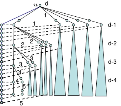
is the degree of the optimal MDMST solution forG. Moreover, this analysis is tight [3].

To illustrate the difficulty of the MDMST problem, we describe here a pathological MSTT in a graphG(seeFig. 1): the treeThas a long path consisting ofO

(

n

)

nodes ending in a nodeuof degreed. The children ofueach have degree

(

d

−

1

)

; the children of the degree-

(

d

−

1

)

nodes have degree

(

d

−

2

)

, and so on until we get to the leaves. Each edge on the path has cost

, and an edge from a degree-

(

d

−

i

+

1

)

node to its degree-

(

d

−

i

)

child has costi. In addition, each of the degree-

(

d

−

i

)

nodes has a cost-iedge to one of the nodes on the path. For somedwithd

=

O

(

logn

/

log logn

)

, the number of nodes in the graph isO

(

n

)

.

Note that an MST ofGwith optimal degree consists of the path along with the non-tree edges and has maximum degree 3. On the other hand, every cost-neutral swap that improves the degree of a degree-

(

d

−

i

)

node in the current tree increases the degree of a degree-

(

d

−

i

−

1

)

node. Hence the treeT is locally optimal for the algorithms of [6,15]. Moreover, all the improving edges are incident on a single component of low-degree nodes; one can verify that the algorithm of Chaudhuri et al. [3] starting with this tree will not be able to improve the maximum degree. In fact, a slightly modified instance,G0_, where several of the non-tree edges are incident on the same node on the path, is not improvable beyondO

(

d

)

. Previous techniques do not discriminate between different nodes with degree less thand

−

1 and hence cannot distinguish between

GandG0_.

On the other hand, our MDMST algorithm, described in Section3, may perform a swap that improves the degree of a degree-dnode by creating one or more new degree-dnodes. In turn, it attempts to improve the degree of these new

degree-Fig. 1.GraphGand a locally optimal tree. The shaded triangles at each level represent subtrees identical to the explicit subtree (on the left) rooted at the same level. The bold nodes represent a path and the bold dotted edges correspond to a set of edges going to similar nodes in the subtrees denoted by shaded triangles.

dnodes, which cannot necessarily be improved independently since their improvements may rely on the same edge or use edges that are incident to the same node. Moreover, this effect snowballs as more and more degree-dnodes are created.

As previously mentioned, Goldberg’s push–relabel framework helps us tame this beast of a process. A high-degree node may only relieve a unit of excess degree using a non-tree edge that is incident to nodes of lower labels. Thus, while two high-degree nodes may be created by a swap, at least they are guaranteed to have lower labels than the label of the node initiating the swap. While the algorithm may end up undoing a previous swap, the labels ensure that this process cannot continue indefinitely.

We define a notion of afeasiblelabeling and prove that our MDMST algorithm maintains one. During the course of the algorithm, there is eventually a labelp∗such that the number of nodes with label at leastp∗is not much larger than the number of nodes with label at leastp∗

+

1. We use feasibility to show that all nodes with labelsp∗and higher must have high average degree inanyMST, thus obtaining a lower bound on∆_opt

(

G

)

. This degree lower bound also holds for any fractional MST of the graphG.

Combining our MDMST algorithm with the cost-bounding techniques of Konemann and Ravi [

¨

15] gives our result for the BDMST problem (Section7).

1.2. Organization of the paper

The rest of the paper is organized as follows. Section2defines the notation used throughout the paper, and Section3 describes our push–relabel algorithm for the MDMST problem. We give two different (and incomparable) bounds on the performance of the algorithm in Sections4and5. In Section5.2, we use a result of Goemans to derive an algorithm with an additive error of 2. Section6generalizes our results to the MDMCB problem. Finally, in Section7, we give our results for the BDMST problem.

2. Definitions and notation

For a graphG

=

(

V

,

E

)

and an MSTT ofG, the degree∆

(

T

)

ofTis defined to be the maximum over nodesuinV, of the degree ofuinT. WhenTis obvious from context, we simply write its degree as∆.

For a subsetF

⊆

Eof edges and a subsetU

⊆

V of nodes, letiF

(

U

)

denote the set of edges inF that have both

endpoints inU, and let

ϑ

F

(

U

)

denote the set of edges inFincident onU, i.e.iF

(

U

)

= {

(

u

, v)

∈

F

:

u

, v

∈

U

}

and

ϑ

F

(

U

)

=

{

(

u

, v)

∈

F

:

u

∈

Uor

v

∈

U

}. Finally,

δ

F

(

u

)

denotes the set of edges inFincident on a vertexu, i.e.

δ

F

(

u

)

= {

e

∈

F

:

u

∈

e

}.

LetNbe the set of nonnegative integers. Alabeling lof the nodes is a functionl

:

V

→

N. For a labelingland an integer

p, letlevel pbe defined as the set

{

v

:

l

(v)

=

p

}

of nodes that have labelp, and letWp

= {

v

:

l

(v)

≥

p

}

be the set of nodes

with labels at leastp. For a real number

µ

≥

1, levelpis called

µ

-sparseif

W_p

≤

µ

W_p+1

.

Given an MSTT, we define aswapinTto be a pair of edges

(

e

,

e0

₎

_{such thate}

_∈

_T,e0

_6∈

_T,c

₍

_e

₎

₌

_c

₍

_e0

₎

_{, andelies on the} unique cycle ofT

∪

e0 _{. Note that if}

₍

_e

_,

_e0

₎

_{is a swap inT, thenT}

_{\ {}

_e

_{} ∪}

e0 _{is also an MST ofG. For a nodeuand a treeT,} letST_udenote the set of swaps

(

e

,

e0

)

inT such thateis incident onuande0is not incident onu. We call a swap

(

e

,

e0

)

inS_uT usefulforubecause it can be used to decrease the degree ofu; i.e. the degree ofuinT

\ {

e

} ∪

e0 _{is one less than that inT.} Given a labelinglonV, we extend it to a labeling onEby definingl

(

e

)

=

max{l

(

u

),

l

(v)

}

fore

=

(

u

, v)

. We say that a labelinglisfeasiblefor a treeT if for all nodesu

∈

V, for every swap

(

e

,

e0

)

∈

S_uT,l

(

e

)

≤

l

(

e0

)

+

1. Given a labelingland an MSTT, a swap

(

e

,

e0

₎

_∈

_ST

uis calledpermissibleforuifl

(

u

)

≥

l

(

e

0

₎

₊

_{1. We show in Section3.2that our algorithm maintains} a feasible labeling. Consequently, each permissible swap

(

e

,

e0

₎

_∈

_ST

u satisfiesl

(

u

)

=

l

(

e

0

₎

₊

_1. We defer the definitions for the MDMCB problem to Section6.1.

Algorithmpr-mdmst

(

G

, µ)

T

←

arbitrary MST ofG. Repeat

∆

←

maximum degree over nodes inT. Initialize labels to 0.

Put excess of 1 on nodes with degree∆. Put excess of 0 on all other nodes. Repeat

p

←

lowest level that contains an overloaded node. Selectthe setUp

←

overloaded nodes with labelp.

Ifthere is a nodeu

∈

Upthat has a permissible, useful swap

(

e

,

e0

)

wheree

=

(

u

, v)

T

←

T

\ {

e

} ∪ {

e0

_};

Set excess on the endpoints ofeto 0; Foreach endpoint ofe0_{that has degree∆.}3

set its excess to 1. else

Relabel all nodes inUptop

+

1.

untilthere are no more overloaded nodes orthere is a

µ

-sparse level. untilthere is a

µ

-sparse levelp∗.

LetF

⊂

T be the edges inT notincident onWp∗₊₁.

Output treeTand the pairWp∗

=

(

F

,

Wp∗

)

.

Fig. 2.A push–relabel algorithm for the MDMST problem. 3. Minimum-degree MSTs

MDMST problem:Given a weighted graphG

=

(

V

,

E

,

c

)

, find an MSTTofGsuch that max_v∈V

{deg

T

(v)

}

is minimized. 3.1. The push–relabel MDMST algorithm

Starting with an arbitrary MST of the graph, our algorithm runs in phases. The idea is to reduce the maximum degree of the tree in each phase using a push–relabel technique. If we fail to make an improvement in some phase, we find a certificate of near-optimality.

More formally, let∆ibe the maximum degree of any node in the treeTiat the beginning of phasei, also called the∆i

-phase. During the∆i-phase, either we modifyTi to getTi+1such that the maximum degree inTi+1is less than∆i, or we

output a certificate that∆iis close to optimal.

For a general phase of the algorithm, letT be the tree at the beginning of the phase, and let∆be the degree ofT. The algorithm maintains a labelingl. The algorithm maintains the invariant that the labelinglis feasible with respect to the current treeT. This notion of feasibility is crucial in establishing a lower bound on the optimal degree when the algorithm terminates.

In addition, each node is given an initialexcess. The excess of a node is one if its degree is∆, and zero otherwise. As we show inLemma 5, the algorithm maintains the invariant that the degree of each node is at most∆. For notational convenience, we call a nodeoverloadedif it has positive excess.

Thepr-mdmstalgorithm takes as input a graphGand a real-valued parameter

µ

≥

1. The parameter

µ

determines

the termination condition of the main loop of the algorithm. In Sections4and5, we derive two different bounds on the approximation ratio of the algorithm; the parameter

µ

is chosen appropriately in the two cases.

We now describe a general phase of the algorithm. SeeFig. 2for a formal description. The phase proceeds as follows: The labell

(

u

)

of each nodeuis initialized to zero. The excess of each node of degree∆is initialized to one; the excess of every other node is initialized to zero.

Letpbe the label of the lowest level containing overloaded nodes. If there is an overloaded nodeuin levelpthat has a permissible, useful swap

(

e

,

e0

₎

_∈

_ST

u, modifyTby deletinge

=

(

u

, v)

and addinge

0

₌

₍

_u0

_{, v}

0

₎

_{. Then decrease the excess on}

uby one; if

v

has positive excess, decrement its excess as well. Ifu0_{now has degree∆or more, add one to its excess; if}

_v

0 has degree∆or more, add one to its excess. If no overloaded node in levelphas a permissible, useful swap, thenrelabelto

p

+

1 all overloaded nodes in levelp. Repeat this loop until either there are no overloaded nodes or there is a

µ

-sparse level. Note that if the phase ends for the former reason, then the tree at the end of the phase has maximum degree at most∆

−

1. In the latter case, we show that∆is close to the optimal degree.

a

b

c

d

Fig. 3.Proof ofLemma 1.

If some node gets labeln, there is guaranteed to be a 1-sparse level. Thus each node gets relabeled at mostntimes per phase, for any choice of the input parameter

µ

≥

1. The total number of iterations of the inner loop in any phase of the algorithm is therefore bounded byn2. Since each phase (except the last) decreases the maximum degree ofTby one, there are at mostnphases. The algorithm therefore runs in polynomial time.

The algorithm outputs a treeTand a pairWp∗

=

(

F

,

X

)

, whereFis a forest onGandXis a subset of nodes. In the rest of this section, we show how to interpret

(

F

,

X

)

as a certificate that the degree ofTis close to∆_opt

(

G

)

. We do this in two different ways, in Sections4and5, leading to two incomparable bounds on the approximation ratio of the algorithm. Remark:In Section4, we set

µ

to a constant larger than 2. In this case, the number of relabels per node is bounded by log₂n, resulting in a faster algorithm.

3.2. Feasibility

We first prove a crucial lemma.

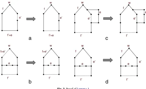
Lemma 1. The algorithm always maintains a feasible labeling.

Proof. We prove this by induction on the number of iterations in a phase. At the beginning of any phase, all labels are zero, which is a feasible labeling. In one step of the algorithm, we either update a label or perform a permissible swap

(

e

,

e0

₎

_{. Since} we increment the label of a node only when it has no permissible swaps, feasibility is maintained in the first case.

In the second case, since we change the structure of the tree, the set of available swaps may change. Consider a feasible swap

(

e

,

e0

₎

_{, wheree}

₌

₍

_u

_{, v)}

_ande0

₌

₍

_u0

_{, v}

0

₎

_{, and the swap is permissible foruor}

_v

_{(or both). LetTbe the tree before the}

(

e

,

e0

₎

_{swap, and letT}0_{be the tree after the swap. Consider a swap}

₍

_f

_,

_f0

₎

_inT0_{. To show that feasibility is maintained, we} need to show thatl

(

f

)

≤

l

(

f0

)

+

1.

If the swap

(

f

,

f0

₎

_{already exists inT, feasibility holds inductively. However, the swap may have been missing in the tree}

T, but may appear in treeT0for one of the following three reasons.

•

f0

_∈

_{T and hence not available for the swap:SeeFig. 3(a). In this case,f}0

₌

_{e. The cycle formed by addingf}0_toT0_includes

e0_{andf, otherwiseT already has a cycle. Moreoverc}

₍

_f

₎

₌

_c

₍

_f0

₎

₌

_c

₍

_e0

₎

_{. Therefore}

₍

_f

_,

_e0

₎

_{is a swap inT, and feasibility} inT implies thatl

(

f

)

≤

l

(

e0

)

+

1. On the other hand, since

(

e

,

e0

)

is a permissible swap inT,l

(

e

)

≥

l

(

e0

)

+

1. Thus

l

(

f

)

≤

l

(

e0

₎

₊

₁

_≤

_l

₍

_e

₎

₌

_l

₍

_f0

₎

_.

•

f

6∈

T and hence not available for the swap:SeeFig. 3(b). In this case,f

=

e0_{. As}

₍

_e

_,

_e0

₎

_{is a swap inT and}

₍

_e0

_,

_f0

₎

_{is a swap} inT0_{, the cycle formed by addingf}0_{toTincludese, and}

₍

_e

_,

_f0

₎

_{is a valid swap inT.l}

₍

_e

₎

_≤

_l

₍

_f0

₎

₊

_{1 by feasibility ofT, and}

l

(

e

)

=

l

(

e0

)

+

1 by permissibility. Thusl

(

f

)

=

l

(

e0

)

≤

l

(

f0

)

.

•

f

∈

T and f0

6∈

T :SeeFig. 3(c) and3(d). Since

(

e

,

e0

)

is a swap inT, there is a unique cycle inT

∪

e0that contains

e. Iff does not lie on this cycle, as illustrated inFig. 3(c), the swap

(

f

,

f0

₎

_{already exists inT and the claim holds} by induction. Otherwise the cycle inT

∪

e0_{containsf, and the only structure in which this happens is illustrated in} Fig. 3(d). Sincee0is the missing edge inT of the cycle inT

∪

e0, it must be the case thatc

(

e0

)

≥

c

(

f

)

=

c

(

f0

)

, or else

T

\ {

f

} ∪ {

e0

}

would have strictly smaller cost than the MSTT. Similarly, sincef0is the missing edge of the cycle inT

∪

f0,

c

(

f0

₎

_≥

_c

₍

_e

₎

₌

_c

₍

_e

₎

_{. Thereforec}

₍

_e

₎

₌

_c

₍

_e0

₎

₌

_c

₍

_f

₎

₌

_c

₍

_f0

₎

_{. Moreover,}

₍

_f

_,

_e0

₎

_and

₍

_e

_,

_f0

₎

_{are both available swaps inT.} Thusl

(

f

)

≤

l

(

e0

₎

₊

₁

₌

_l

₍

_e

₎

_≤

_l

₍

_f0

₎

₊

_1.

We have shown that, in all cases, the swap

(

f

,

f0

₎

_{is feasible. Hence the induction holds.}

3.3. The witness

In this section, we introduce the notion of awitness. A witness is a combinatorial structure produced by our algorithms at termination to guarantee the near-optimality of the output. Our witness consists of a forestF

⊆

Ethat is contained in some MST ofG, along with a subsetX

⊂

V. A pair

(

F

,

X

)

is a witness if it has the following property: For every MSTTofG

containingF, every edge inT

\

Fis incident onX.

Lemma 2 ([6]).LetW

=

(

F

,

X

)

be a witness for a graph G

=

(

V

,

E

)

as defined above. Then any (fractional) minimum spanning tree of G has maximum degree at least|V|−|_|XF_||−1.

Proof. Consider an MSTTofG, and letT0be an MST containingFthat has maximal intersection withT. By the exchange property,T0

_\

_{Fis contained inT. The witness property implies that every edge inT}0

_\

_{Fis incident onX. Since there are}

|

V

| − |

F

| −

1 edges inT0

\

F, the average degree ofXinT0

\

F, and therefore inT, is at least|V|−|_|XF_||−1. Since a fractional MST is a convex combination of integral ones, the claim follows.

We now show that the pair

(

F

,

X

)

output by the algorithmpr-mdmstis a witness.

Lemma 3. Let T be the MST of G and l

:

V

→

Nthe labeling when the algorithmpr-mdmstterminates. For any integer p, let F be the subset of edges in T that are not incident on Wp+1, and let X

=

Wp. ThenWp

=

(

F

,

X

)

is a witness.

Proof. Assume the contrary, and letT0be an MST ofGthat containsFand also contains an edgee0

6∈

Fnot incident onWp.

By the exchange property, there is an edgee

∈

T

\

Fsuch that

(

e

,

e0

₎

_{is a swap inT. Sincee}

_∈

_T

_\

_{F, it is incident onW}

p+1

and thusl

(

e

)

≥

p

+

1. On the other hand,e0_{is not incident onW}

pand thusl

(

e0

)

≤

p

−

1. This, however, contradicts the

feasibility of the labeling. 3.4. Involuntary losses

Letp∗_{be the}

_µ

_{-sparse level used by the algorithm to compute a witness. FromLemma 2andLemma 3, it follows that any} (fractional) MST ofGhas degree at least|V|−| F|−1

Wp∗

. This ratio can be rewritten as(|V|−|F|−1) Wp∗ +1

·

Wp∗ +1 Wp∗

. Note that the numerator of the first term is precisely the number of edges incident onWp∗₊₁inT. The second term is bounded by1

µ, where

µ

is the sparseness of levelp∗. The next lemma follows immediately.

Lemma 4. Let T be the MST of G, l

:

V

→

Nthe labeling, and p∗the

µ

-sparse level when the algorithmpr-mdmstterminates. Let

ϑ

T

(

Wp∗₊₁

)

be the set of edges in T incident on W_p∗₊₁. Then any (fractional) MST of G has degree at least 1

µ

·

ϑT(Wp∗ +1) Wp∗ +1 .

Thus, to prove a lower bound on∆_opt

(

G

)

, we need to lower bound

ϑ

T

(

Wp∗+1

)

. Towards this end, we distinguish between two different ways a node can lose degree during the course of the algorithm.

We say that a swap

(

e

,

e0

₎

_{executed by the algorithmcausesa loss in degree to a nodeuifeis incident onu. A loss in degree} to a nodeuthat is caused by a swap

(

e

,

e0

)

is called avoluntary lossifuis overloaded before the swap is executed; otherwise it is called aninvoluntary loss. By definition, voluntary losses do not decrease the degree of a node below∆

−

1. Note that every swap

(

e

,

e0

₎

_{executed by the algorithm causes a voluntary loss to at least one endpoint ofe(and an involuntary loss to} at most one endpoint ofe).

Suppose the algorithm terminates with a

µ

-sparse level in the∆-phase. The last time it is relabeled, each node inWp∗₊₁

has degree at least∆and is therefore overloaded. If each node inWp∗₊₁suffered only voluntary losses in degree since its

last relabeling, then its degree inTwould be at least∆

−

1. However, a node inWp∗₊₁may also suffer from involuntarily

losses, which may decrease its degree arbitrarily. Hence a node-by-node analysis is insufficient. To get a lower bound on the average degree ofWp∗₊₁inT, we instead bound the total number of involuntary losses to nodes inW_p∗₊₁. We do this in two

different ways in the next two sections. 4. A constant-factor approximation

In this section, we show that the algorithm outputs a treeTof degree∆

≤

2∆_opt

(

G

)

+

O

(

√

∆

)

. To bound the number of involuntary losses, we define a partitioning of the swaps executed by the algorithm intocascades. Each cascade can be charged to a relabel, which enables us to bound the number of involuntary losses toWp∗₊₁in terms of the size of this set. 4.1. Cascades

Recall that, for an integerp,Upis defined to be the set of overloaded nodes in levelp. For the purpose of analysis, we

removed. In addition, we give each node anoverloading-swapfield. The overloading-swap field of a nodeupoints to the swap that put excess on it after its last relabel. We start with all the flags cleared and all overloading-swap fields set to null. In each iteration of the∆-phase of the algorithm, we find the lowestpsuch thatUpis non-empty, i.e. there is an overloaded

node with labelp. If we can find any swap

(

e

,

e0

)

that is permissible and useful for a node inUp, we execute the swap and

clear flags (if set) on the endpoints ofe. Moreover, for each endpointu0_ofe0_{that is now overloaded, we set the} overloading-swap field ofu0_to

₍

_e

_,

_e0

₎

_{. If there is no swap that is permissible and useful for any node inU}

p, we increment the label, set

the flag, and clear the overloading-swap field for each node inUp.

The following lemma shows that no node has excess larger than one during the course of the algorithm, which implies, in particular, that the overloading-swap field is never overwritten before it is cleared to null.

Lemma 5. During the∆-phase, no node ever has degree more than∆.

Proof. We use induction on the number of swaps executed during the phase. In the beginning of the phase, the maximum degree is∆. Any swap

(

e

,

e0

)

decreases the degree of a node inUpand adds at most one to the degree of a node with strictly

lower label. By choice ofp, all nodes with lower labels have degree at most∆

−

1 before the swap. Since a swap adds at most one to the degree of any vertex, the induction holds. The lemma follows.

We define thelabel of a swap

(

e

,

e0

)

to be the label ofewhen the swap is executed. We call a swap aroot swapif it is useful for a flagged node. Note that a flagged node has its overloading-swap field set to null. Let

(

e

,

e0

₎

_{be a non-root swap} that occurs in the sequence of swaps executed by the algorithm. The swap

(

e

,

e0

₎

_{is executed in order to relieve the excess of} an endpointuofe. Let

(

f

,

f0

)

be the swap pointed to by the overloading-swap field for nodeuwhen swap

(

e

,

e0

)

is executed. Thus

(

f

,

f0

₎

_{is the last swap in the sequence that increases the degree ofuand precedes}

₍

_e

_,

_e0

₎

_{. We call}

₍

_f

_,

_f0

₎

_{theparent swap} of

(

e

,

e0

₎

_{. Note that the flagging procedure ensures that every non-root swap executed by the algorithm has a parent.}

A label-pswap, by definition, reduces the degree of a node with labelp. Since excess flows from a higher-labeled node to a lower-labeled node, the label of every non-root swap is strictly smaller than the label of its parent. The parent relation naturally defines a directed graph on the set of swaps, each component of which is an in-tree rooted at one of the root swaps. We define acascadeto be the set of swaps in a component of this Directed Acyclic Graph. In other words, a cascade corresponds to the set of swaps sharing the same root swap as an ancestor. Note that the cascades may be interleaved in the sequence of swaps executed by the algorithm. Thelabel of a cascadeis defined to be the label of the root swap in it.

Each swap is the parent of at most two swaps which each have a strictly smaller label. Thus it follows that: Lemma 6. A label-p cascade contains at most2p−q_{label-q swaps.}

We say that an involuntary loss iscontainedin a cascade if some swap in the cascade causes it. Since each swap causes at most one involuntary loss, the lemma above implies:

Corollary 7. A label-p cascade contains at most

(

2p−q+1

₋

₁

₎

_{involuntary losses to nodes with labels at least q.}

Proof. An involuntary loss to a label-rnode must be caused by a swap with label at leastr. The bound follows by summing the number of swaps with labelr, forrbetweenqandp.

4.2. Computing the approximation ratio

Armed with the bound ofCorollary 7, we now proceed to lower bound∆_opt

(

G

)

. Recall from Section3.4that it suffices to lower bound the average degree ofWp∗₊₁inT, whereW_p∗is a

µ

-sparse level andT is the tree output by the algorithm.

Lemma 8. Let p be an integer greater than p∗_{. Then}

Wp

> µ

Wp+1

.

Proof. Each iteration of a phase of the algorithm decreases the size of at most one levelpand increases the size of the level

p

+

1. Thus the only level that can go from not being

µ

-sparse to being

µ

-sparse is levelp. Since the algorithm terminates as soon as it finds a

µ

-sparse level, it terminates with exactly one

µ

-sparse level.

Lemma 9. The number of involuntary losses to nodes in Wp∗₊₁is at most2|W_p∗₊₁

|

(

µ

µ−2

)

.

Proof. Each involuntary loss to a node inWp∗₊₁occurs in a cascade, and byCorollary 7, the number of involuntary losses

to nodes inWp∗₊₁in a label-pcascade is at most 2p−p ∗

. The total number of involuntary losses to nodes inWp∗₊₁during the

course of the phase is at most

X

p≥p∗₊₁ 2p−p∗

|

Wp

|

<

X

p≥p∗₊₁ 2p−p∗

W_p∗₊₁

µ

p−p∗₋₁

=

2

W_p∗₊₁

X

p≥p∗₊₁

2

µ

p−p∗−1

=

2|Wp∗₊₁

|

µ

µ

−

2

.

We are now ready to establish the approximation ratio of the algorithm.

Theorem 10.Given a graph G and a constant

µ >

2, thepr-mdmstalgorithm obtains in polynomial time an MST of degree∆, where∆

≤

µ

∆_opt

(

G

)

+

2

+

_µ2µ

−2.

Proof. Thepr-mdmstalgorithm, when executed on graphG, terminates with a treeT and a pairWp∗

=

(

F

,

X

)

. We now compute the number

ϑ

T

(

Wp∗₊₁

)

of edges incident onWp∗₊₁inT. Each node inW_p∗₊₁has degree at least

(

∆

−

1

)

after its

last voluntary loss, and it may then suffer some involuntary losses. Using the bound fromLemma 9, the sum of degrees of nodes inWp∗₊₁inTis at least

(

∆

−

1

−

2µ

µ−2

)

|

Wp∗+1

|. Since there are at most

W_p∗₊₁

−

1 edges inTthat have both endpoints inWp∗₊₁, the number of edges inTthat are incident onW_p∗₊₁is at least

(

∆

−

2

−

2µ

µ−2

)

|

Wp∗+1

|. Thus from

Lemma 4, ∆opt

(

G

)

≥

∆

−

2

−

2

µ

µ

−

2

1

µ

.

Rearranging, we get ∆

≤

µ

∆_opt

(

G

)

+

2

+

2

µ

µ

−

2

.

Setting

µ

to be 2

+

√

2 ∆_opt(G), we get ∆

≤

2∆_opt

(

G

)

+

4

p

∆_opt

(

G

)

+

4

Corollary 11. Given a graph G, there is a polynomial-time algorithm that outputs an MST of degree∆, where∆

≤

2∆_opt

(

G

)

+

O

(

√

∆_opt

(

G

))

.

5. An additive approximation

In this section, we show a different upper bound on the performance of the algorithm that is better than the bound in the previous section if the graphGiseverywhere-sparse, i.e. for every subsetUof nodes, the induced subgraph onUis sparse.

More precisely, for a graphG, let thelocal density s

(

G

)

be defined as the density of the densest subgraph ofG:s

(

G

)

=

maxU⊂V

n

|iE(U)|

|U|

o

. We show that on inputGand

µ

=

1, thepr-mdmstalgorithm outputs an MST of degree at most∆_opt

(

G

)

+

s

(

G

)

. In Section5.2, we combine this result with a lemma from Goemans [8] to get a

(

∆_opt

(

G

)

+

2

)

-algorithm.

5.1. A density-based bound

LetT be the tree andWp∗_{the witness output by the}

pr-mdmstalgorithm on inputGand

µ

=

1. Let∆be the degree of T. Since

µ

=

1, the setsWp∗ andW_p∗₊₁must be equal, and hence, levelp∗is empty when the algorithm terminates. The

following lemma bounds

ϑ

_T

(

W_p∗₊₁

)

.

Lemma 12. Let T be the MST, l the labeling, and p∗_{the empty level when the algorithm}

pr-mdmstterminates. Let iE

(

Wp∗₊₁

)

be the set of edges in G that have both endpoints in Wp∗₊₁, and let

ϑ

_T

(

W_p∗₊₁

)

be the set of edges in T that are incident on W_p∗₊₁. Then

ϑ

T

(

Wp∗₊₁

)

≥

(

∆

−

1

)

Wp∗₊₁

+

1

−

iE

(

Wp∗₊₁

)

.

Proof. For a nodeu

∈

Wp∗₊₁, let

δ

_T

(

u

)

⊂

Tbe the set of edges inTincident onu, and let

δ

_L

(

u

)

⊂

Ebe the set of edges that

nodeuloses involuntarily after its last voluntary loss. Since each node has degree at least∆

−

1 after its last voluntary loss, it follows that

|

δ

_T

(

u

)

| ≥

∆

−

1

− |

δ

_L

(

u

)

\

δ

_T

(

u

)

|. Moreover, if

v

is the last node to be relabeled,

|

δ

_T

(v)

| ≥

∆. Thus the sum of degrees of nodes inWp∗₊₁inTis at least

(

∆

−

1

)

W_p∗₊₁

+

1

−

P

u∈Wp∗ +1

|

δ

L

(

u

)

\

δ

T

(

u

)

|.

An edge

(

u

, v)

may be in

δ

L

(

u

)

or

δ

L

(v)

but not both. It follows that

P

u∈Wp∗ +1

|

δ

L

(

u

)

\

δ

T

(

u

)

| ≤

∪

u∈Wp∗ +1

(δ

L

(

u

)

\

δ

T

(

u

))

. Recall that every involuntary loss to a node inWp∗₊₁ comes from an edge ini_E

(

W_p∗₊₁

)

. Thus each edge in

∪

_u∈W

p∗ +1

(δ

L

(

u

)

\

δ

T

(

u

))

is iniE

(

Wp∗₊₁

)

\

i_T

(

W_p∗₊₁

)

.

An edge

(

u

, v)

iniT

(

Wp∗₊₁

)

contributes to both

δ

_T

(

u

)

and

δ

_T

(v)

. Thus the number of edges inTincident onW_p∗₊₁is

X

u∈Wp∗ +1

|

δ

_T

(

u

)

| −

i_T

(

W_p∗₊₁

)

≥

(

∆

−

1

)

W_p∗₊₁

+

1

−

∪

u∈Wp∗ +1

(δ

L

(

u

)

\

δ

T

(

u

))

−

i_T

(

W_p∗₊₁

)

≥

(

∆

−

1

)

W_p∗₊₁

+

1

−

i_E

(

W_p∗₊₁

)

\

i_T

(

W_p∗₊₁

)

−

i_T

(

W_p∗₊₁

)

≥

(

∆

−

1

)

W_p∗₊₁

+

1

−

i_E

(

W_p∗₊₁

)

.

We now use the bound on

ϑ

_T

(

W_p∗₊₁

)

inLemma 12to prove a lower bound on∆_opt

(

G

)

. Theorem 13. Let T andWp∗_{be the output of the}

pr-mdmstalgorithm given a graph G and

µ

=

1. Then the degree∆of T is bounded by∆_opt

(

G

)

+

s

(

G

)

.

Proof. ByLemma 12,

ϑ

_T

(

W_p∗₊₁

)

≥

(

∆

−1

)

W_p∗₊₁

+

1

−

i_E

(

W_p∗₊₁

)

. By the definition of local density,

iE(Wp∗ +1) Wp∗ +1

≤

s

(

G

)

. Lemma 4then implies that∆_opt

(

G

)

≥

∆

−

s

(

G

)

−

1

+

1

Wp∗ +1

. Since∆_opt

(

G

)

is an integer, we conclude that∆_opt

(

G

)

≥

∆

−

s

(

G

)

.

5.2. An additive factor of 2

Goemans [8] shows that the support of the natural linear program from the MDMST problem is sparse. He considers the following linear program:

min c

(

x

)

=

X

e cexe subject to: x

(

iE

(

S

))

≤ |

S

| −

1 S

⊂

V x

(

E

)

= |

V

| −

1 x

(δ

E

(v))

≤

k

v

∈

V xe

≥

0 e

∈

E

The above linear program is feasible for an integerkif and only if∆_opt

(

G

)

≤

k. Letx∗_{be an optimal extreme-point} solu-tion to the above linear program for a graphGand fork

=

∆_opt

(

G

)

. LetE∗denote the support ofx∗, i.e.E∗

= {

e

∈

E

:

x∗_e

>

0}. Theorem 5 in Goemans [8] can be paraphrased as:

Theorem 14 (Goemans [8, Theorem 5]). The local density of the graph G∗

₌

₍

_V

_,

_E∗

₎

_{is less than2.} We first argue that∆_opt

(

G

)

=

∆_opt

(

G∗

₎

_{. Sincex}∗

e

=

0 for alle

6∈

E

∗_{, it follows thatx}∗_{is a feasible solution to the linear} program forG∗

₌

₍

_V

_,

_E∗

₎

_{, and so∆}

opt

(

G∗

)

≤

∆opt

(

G

)

. SinceG∗is a subgraph ofG,∆opt

(

G∗

)

≥

∆opt

(

G

)

. We conclude that∆_opt

(

G

)

=

∆_opt

(

G∗

)

.

Since the linear program can be solved efficiently (see, e.g., Schrijver [21], Section 40.3), we can compute the graphG∗_in polynomial time. Our

(

∆_opt

(

G

)

+

2

)

-algorithm computes the graphG∗_{and then runs the algorithm}

pr-mdmstwith input

G∗and

µ

=

1. ByTheorem 13, the treeToutput by the algorithm has degree most∆_opt

(

G

)

+

2.Theorem 15summarizes. Theorem 15. Given a graph G, there is a polynomial-time algorithm that computes an MST of G with degree at most∆_opt

(

G

)

+

2.

6. Minimum-degree minimum-cost base in a matroid

In this section, we consider a generalization of the MDMST problem.

6.1. Definitions

Recall that amatroidis defined to be a pairM

=

(

E

,

I

)

, whereEis a ground set of elements andIis a family ofindependent setssuch that (i)

∅ ∈

I, (ii)A

∈

I,B

⊆

Aimply thatB

∈

I, and (iii)A

,

B

∈

I,

|

A

|

>

|

B

|

imply that there existse

∈

A

\

Bwith

B

∪ {

e

} ∈

_I. A maximum-cardinality independent set ofMis called abaseofM.

Let c

:

E

→

_R+_{be a non-negative cost function on the ground set ofM. A baseT ofM that minimizes the cost}

c

(

T

)

=

P

e∈Tc

(

e

)

is referred to as aminimum-cost base(MCB). LetxT

∈ {0

,

1}

|E|

be the incidence vector of an MCBT. We say a vectorx

∈ [0

,

1]|E|

is a fractional MCB if it is the convex combination of incidence vectors of MCB’s.

Recall that a hypergraphG

=

(

V

,

E

)

consists of a set of nodesVand hyperedgesE

⊆

22V, i.e. each hyperedge is a subset of vertices. We sayGis ak-ary hypergraph if the cardinality of each edge inEis at mostk. Ifu

∈

e, we say that nodeuis an

endpointofeand thateisincidentonu. For a subsetF

⊆

Eof edges and a nodeu

∈

V, let

δ

F

(

u

)

be the set

{

e

∈

F

:

u

∈

E

}

of

edges incident onu. We define thedegree of uinFto be

|

δ

_F

(

u

)

|. The

degree of Fis then defined as the maximum overu

∈

V

of the degree ofuinF, i.e. maxu

|{

e

∈

F

:

u

∈

e

}|

. Further, for a subset of verticesU

⊆

V, letiF

(

U

)

and

ϑ

F

(

U

)

denote the sets

{

e

∈

F

:

e

⊂

U

}

and

{

e

∈

F

:

e

∩

U

6= ∅}, respectively.

We can now formally define the minimum-degree minimum-cost base (MDMCB) problem. The input to the problem is ak-ary hypergraphG

=

(

V

,

E

)

and a matroidMwithEas its ground set.