SIMULTANEOUS CALIBRATION OF MULTIPLE CAMERA HEADS WITH FIXED BASE CONSTRAINT

SIMULTANEOUS CALIBRATION OF MULTIPLE CAMERA HEADS WITH FIXED

BASE CONSTRAINT

A. M. G. Tommaselli a, _{*, M. Galo} a_{, W. L. Bazan} b,c_{, R. S. Ruy} b,d_{, J. Marcato Junior} d a _{São Paulo State University, Dept. of Cartography, 19060-900, Pres. Prudente, S.P., Brazil,}

(tomaseli, galo)@fct.unesp.br

b _{Pos-Graduate Program in Cartographic Sciences ([email protected])} c _{Santiago & Cintra Consultoria ([email protected])}

d _{Engemap Geoinformação ([email protected])}

Commissions V and I, IC WG V/I

KEY WORDS: Dual head cameras, camera calibration, multi frame images.

ABSTRACT:

Image acquisition systems based on multi-head arrangement of digital cameras are attractive alternatives enabling larger imaging area when compared to a single frame digital camera. Besides that, acquisition of multiespectral imagery is easier when independent cameras are used. Considering that in multicamera systems the heads are tightly attached to an external mount, it can be supposed that relative position and orientation between cameras are stable during image acquisition. This work presents an approach based on simultaneous calibration of two or more cameras using constraints stating that the relative rotation matrix and the base distance between the cameras heads are stable. Experiments with images acquired by an arrangement of two Hasselblad H3D cameras were accomplished with terrestrial calibration field. The experiments have shown that the calibration technique with RO constraints allows advantages when compared to the approach based on single camera calibration.

1. INTRODUCTION

Recent developments in the technology of optical digital sensor made available digital cameras with medium format at reasonable costs, when compared to high-end digital photogrammetric cameras. Due to this favorable cost/benefit ratio, many companies has been adapted professional medium format cameras for use in mapping and general photogrammetric tasks (Habib and Morgan, 2003; Roig et al, 2006; Ruy et al, 2007).

When compared to a classic photogrammetric film cameras (23x23cm format), however, digital medium format cameras present small ground coverage area. Modern photogrammetric digital cameras overcome this drawback with distinct approaches: multiple linear pushbroom sensors (DLR HRSC, Leica ADS 40) or multiple frame camera heads (Z/I DMC, Vexcel Ultracam, DIMAC).

Image acquisition systems based on multi-head arrangement of digital cameras are attractive alternatives enabling larger imaging area when compared to a single digital frame camera. Acquisition of multiespectral imagery is facilitated when considering independent cameras. Several manufactures are following this tendency, integrating individual cameras to produce high-resolution multiespectral images. Independent developers also are integrating their own low cost systems with small and medium format off-the-shelf cameras (Roig et al, 2006; Ruy et al, 2007). These images can be processed as units (Mostafa and Schawarz, 2000) or they can registered and mosaicked to generate a high resolution multispectral image. In any case, the knowledge of relative orientation between cameras is desirable.

One strategy is to directly measure the coordinates of the perspective centers of each individual camera and to determine indirectly the orientation (rotation matrix) of these cameras by a bundle block adjustment (Doerstel et al., 2002).

Another alternative, presented in this paper, is the simultaneous calibration of two or more cameras using constraints stating that the relative rotation matrix and the base distance between the cameras heads are stable. An additional constraint can also be introduced with the measured length between the external nodal points.

This approach is assessed with close range images and some experiments are presented showing the feasibility and advantages of the process over the individual calibration of each head.

2. BACKGROUND 2.1 Camera Calibration

Camera calibration aims at the determination of a set of IOP - inner orientation parameters (focal length, principal point coordinates and lens distortion) (Brown, 1971; Merchant, 1979, Clarke and Fryer, 1998; Cramer, 2004; Mikhail et al, 2001). This process can be carried out by several methods: laboratory methods, like goniometer or multicolimator; stellar and field methods like mixed range field, convergent cameras and self calibrating bundle adjustment. In the field methods, image observations of points or linear features in several images are used to indirectly estimate the IOP by bundle adjustment with Least Squares Method. The mathematical model used are the collinearity equations with additional parameters (Eq. 1).

0 = Q N f + Δy -0 y -F y = 2 F 0 = Q M f + Δx -0 x -F x = 1 F (1)

where xF, yF are the image coordinates; M, N, Q, Δx and Δy are obtained by: ) Z -(Z m + ) Y -(Y m + ) X -(X m M _{11 0 12 0 13 0} ) Z -(Z m + ) Y -(Y m + ) X -(X m N 21 0 22 0 23 0 ) Z (Z m + ) Y (Y m + ) X (X m Q _{31 0 32 0 33 0} Δx = a d r δx δx δx + + , Δy = a d r δy δy δy + + ;

and

m

_ij are the rotation matrix elements.

In these equations the radial and decentering lens distortion coefficients are given by Eq(s). (2) and (3) (Brown, 1966):

) y -...)(y r k + r K + r (K = δy ) x -...)(x r K + r K + r (K = δx 0 6 3 4 2 2 1 0 6 3 4 2 2 1 r r ₍₂₎

where r is the radial distance related to the principal point.

] ) y -2(y + [r P + ) y -)(y x -(x 2P = δy ) y -)(y x -(x 2P + ] ) x -2(x + [r P = δx 2 0 2 2 0 0 1 0 0 2 0 2 1 d 2 d ₍₃₎

Affinity parameters can be estimated with Eq. (4) (Moniwa, 1972; Habib e Morgan, 2003). ) 0 y -A(y = a δy ) 0 y -B(y ) 0 x -A(x = a δx  (4)

where A and B are the affinity parameters.

The method of calibration using bundle adjustment is based on the collinearity equations (Eq. (1)) and distortion models (Eq(s). (2), (3) and (4). In this method the exterior orientation parameters (EOP), interior orientation parameters (IOP) and object coordinates of photogrammetric points are simultaneously estimated from image observations and some additional constraints. This method can be used with no control points given a minimum of seven constraints to define an object reference frame; this particular approach is known as self-calibrating bundle adjustment (Merchant, 1979).

In this method a linear dependence between parameters arises when the camera inclination is near zero and the flight height has little variation. In these cases, focal length (f) and flight height (Z–Z0) are not separable and the system equation became singular or ill conditioned. Besides theses correlations, also the coordinates of the principal point are highly correlated to the perspective center coordinates (x0 and X0; y0 and Y0). In order to cope with these dependences, several methods were proposed like the mixed range method (Merchant, 1979) and the convergent cameras method (Brown, 1971).

Multihead and stereo camera calibration

Previous works on stereo or multi-head calibration usually do not take advantage of stability constraints (Zhuang, 1995; Doerstel, 2002).

Considering that in multicamera systems the heads are tightly attached to an external mount, it can be supposed that relative position and orientation between cameras are stable during image acquisition. As a consequence, some additional constraints related with this geometry can be included in the calibration step, when using bundle adjustment. The inclusion of these constraints in a bundle adjustment seems to be relevant since the estimation of relative orientation (RO) parameters from a previous adjusted block shows significant deviations between different pair of images, i.e., larger physical variations than the expected ones.

In order to solve this problem, this work presents an approach based on simultaneous calibration of two or more cameras using constraints stating that the relative rotation matrix and the base distance between the cameras heads are stable. An additional constraint is also introduced with the measured length between the external nodal points.

2.1 Parameter estimation with Least Squares Method Collinearity equations combine adjusted observations (La) and unknowns (Xa) in an implicit model, which can be represented as F(La,Xa)=0, and the linearized model takes the following form (Mikhail and Ackerman, 1976):

0

W

AX

BV







(5) where A is the design matrix related to the parameters, B is the design matrix related to the adjusted observations, V is the vector of residuals, X is the vector of corrections to the approximated parameters and W is a misclosure vector.

Let us consider now a set of constraints equations taking the form:

_F

_c

₍

_L

a_c

_,

_X

_a

₎



₀

. The corresponding linearized equations are:

0









CX

W

V

B

C C (6) where La

c are “pseudo-observations”, Bc is the design matrix of functions Fcwith respect to this pseudo-observations, C is the design matrix of functions Fc with respect to the parameters and

W’ also a misclosure vector:

)] X , L ( F ) L L ( B [ W b 0  0 0 and W [Bc(Lc Lc) Fc(Lc,X0)] 0 0 _   

The vector of corrections to the approximated parameters is given by, which is updated with iterations:

)] (U+U [σ )] (N+N σˆ X=-[ c 2 0 1 -c 2 0 (7) where N AT(BQBT)-1A and _UAT_(BQBT₎-1_W C ) B Q (B C N T -1 c c c c T  and _{U C (BQB}T₎-1_W' c c c c T 

In case the value of a parameter is previously known, with certain accuracy, for example, the coordinates of control points, then a weighted constraint can be applied.

3. RELATIVE ORIENTATION CONSTRAINTS AND GEOMETRY OF THE DUAL-HEAD SYSTEM As described in Section 1, the central point of this paper is concerned with the analysis of the RO constraints applied to a dual-head digital imagery system, assuming that the system is physically stable during the image acquisition flight mission. Before developing the proposed method, the geometry of the dual-head system will be briefly described.

3.1 The geometry of a dual-head system: SAAPI

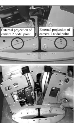
The SAAPI system (Ruy et al, 2007) is composed of two Hasselblad digital cameras, positioned in a convergent way, as shown in Figure 1. The images can be acquired simultaneously with a fixed superposition.

The elements Κ, Φ e Ω are the relative orientation (RO) angles, considering as reference the right camera (C1) and D is the Euclidian distance between C1 and C2. The approximated values of the angles Ω, Φ e K are of -36º, 0º and 180º, respectively.

The RO elements can be calculated as function of the exterior orientation parameters (EOP) of both cameras by using:

 

1 2 1  R R R_RO (8)

where RRO are the RO matrix, corresponding to the angles K, Φ,

and Ω; R1and R2 are rotation matrix for the cameras 1 and 2, respectively. Another element that can be considered as stable during the acquisition is the Euclidian distance D between the perspective centers. This distance can be directly measured, since the location of the external nodal points can be obtained from the technical data provided by the camera and lens manufactory (Figure 1.b).

a)

External projection of camera 2 nodal point

External projection of camera 1 nodal point

b)

Figure 1. PC’s projected to the external mount (a) and measurements of the PC distance (b).

3.2 Dual-head calibration method

In the proposed method, the basic mathematical model for calibration of the dual-head system are the colinearity equations (Eq. 1) with additional parameters and the constraints equations developed in this section.

Let t RO

R

be the RO matrix and 2 t

D the squared distance between the cameras perspective centers, for the instant t and, analogously, for the instant t+1,

R

_ROt1 and 2

1 t

D. As previously

mentioned, it is reasonable to consider the RO matrix and distance between the perspective centers stable, although the orientation of each camera changes. Based on these assumptions, the following equations can be written:

0 = R -R_ROt t_RO+1 (9) 0 D D t21 2 t    (10) with: (t) t RO ) r r + r r + r (r ) r r + r r + r (r ) r r + r r + r (r ) r r + r r + r (r ) r r + r r + r (r ) r r + r r + r (r ) r r + r r + r (r ) r r + r r + r (r ) r r + r r + r (r = R 2 33 1 33 2 32 1 32 2 31 1 31 2 23 1 33 2 22 1 32 2 21 1 31 2 13 1 33 2 12 1 32 2 11 1 31 2 33 1 23 2 32 1 22 2 31 1 21 2 23 1 23 2 22 1 22 2 21 1 21 2 13 1 23 2 12 1 22 2 11 1 21 2 33 1 13 2 32 1 12 2 31 1 11 2 23 1 13 2 22 1 12 2 21 1 11 2 13 1 13 2 12 1 12 2 11 1 11          

where

r

_ijcamera are the elements of rotation matrix for both camera, with i,j={1, 2, 3}.

Considering the Equations (9) and (10), based on the EOP for both camera in consecutive instants, t and t+1, three linearly equations can be written:

0 = ) r r + r r + r (r ) r r + r r + r (r = G (t)- (t 1) 1 2 13 1 23 2 12 1 22 2 11 1 21 2 13 1 23 2 12 1 22 2 11 1 21  ₍₁₁₎ 0 = ) r r + r r + r (r -) r r + r r + r (r = G (t) (t 1) 2 2 13 1 33 2 12 1 32 2 11 1 31 2 13 1 33 2 12 1 32 2 11 1 31  ₍₁₂₎ 0 = ) r r + r r + r (r -) r r + r r + r (r = G (t) (t 1) 3 2 23 1 33 2 22 1 32 2 21 1 31 2 23 1 33 2 22 1 32 2 21 1 31  ₍₁₃₎ -) Z -(Z + ) Y -(Y + ) X -(X = G 01 2 2 0 2 1 0 2 0 2 1 0 2 0 (t) (t) (t) (t) (t) (t) 4 0 = ) Z -(Z -) Y -(Y -) X -(X₀2(t+1) ₀1(t+1) 2 ₀2(t+1) ₀1(t+1) 2 ₀2(t+1) ₀1(t+1) 2 (14) The direct measurement of the physical distance among PCs with a pachymeter resulted in the observed value of 111,200 mm ± 1 mm. Then, besides of the four constraint Eq(s) (11) to (14), one additional constraint equation based in the measured distance can be included. In fact, it’s is important to mention that the precision expressed in the measured distance is not related to the pachymeter itself but mainly by the projection of the PC to the external mount.

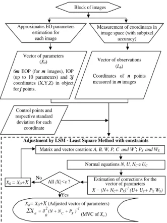
The mathematical models corresponding to the mentioned constraints were implemented using the C/C++ language on the CMC (Calibration of Multiple Cameras) program (Ruy et al, 2007). The flowchart in the Figure 2 shows the main process steps implemented based in the previous models.

Figure 2. Flowchart of the proposed method.

4. EXPERIMENTS AND RESULTS ANALYSIS In order to assess the proposed methodology, four experiments were carried out, without and with RO constraints, and with different weights for these constraints (Table 1).

In the experiments fourteen images were used (seven of each camera) resulting in 2606 image observations (Figures 3b and 3c) corresponding to circular targets and other distinguishable features (corners) in the test field (Figure 3a). The image coordinates of circular targets were extracted with subpixel accuracy using an interactive tool that computes the mass center after automatic threshold estimation. The coordinates of other points like corners of painted letters were extracted manually, and thus, their accuracy are of pixel level.

Four exposure stations were used and in each station 4 images were taken (2 for each camera), with the dual-mount being rotated by 90º. Due to the physical dimensions of the test field and to the camera depth of field and coverage angle, in some images few targets were acquired. For this reason, only 14 images from 29 originally acquired could be used.

From this group of 14 images, 5 of each camera were taken at the same instant, and then, constraints equations can be stated

for these pairs. The group of 671 parameters estimated in the Least Squares Estimation is composed by: 6 EOP for each image; 10 IOP for each camera; 3 coordinates for each point in the object space (total of 189 points). In this set of points, 27 were used as control points, 44 as check points and the remaining were considered photogrammetric points. The a priori variance was stated as a 2.025E10-5 _mm2_{, corresponding} to a standard deviation of 0.5 pixel (0.0045mm) in the image coordinates. The image coordinates were weighted depending on the type of measurement: 0.5 pixel for circular targets and 1 pixel for the points measured manually.

(a)

(b) (c)

Figure 3. (a) Test field and distribution of image points in images taken with cameras 1 (b) and 2 (c).

The weights in the pseudo-observations of the constraints Eq(s). (11, 12 and 13), were computed by covariance propagation, based on the admitted variations for each angular element. The smaller are the admitted variations the higher are the weights in the constraints.

Figure 4 presents the absolute values of residuals in the observation after least squares adjustment for experiments A

(a) (b) 0,00E+00 1,00E-06 2,00E-06 3,00E-06 A B C D Experiments A p o st er io ri v ar ian ce (c)

Figure 4 – Absolute value of residuals in the observations for experiments A (a) and C (b), and a posteriori variance for all experiments (c) (units are pixels).

Vector of parameters (X0)

6m EOP (for m images), IOP (up to 10 parameters) and 3j

coordinates (X,Y,Z) in object for j points.

Normal equations N, U, NCe UC

Yes No

Matrix and vector creation: A, B, W,P, C and W’; PX and WX

Measurement of coordinates in image space (with subpixel

accuracy) Approximates EO parameters

estimation for each image

Estimation of corrections for the vector of parameters

X = (N+ NC+ PX)-1 (U+ UC+ PX WX)

All |Xi|<ε ?

Xa= X0+X (Adjusted vector of parameters) 1 -2 0 a=σ (N+NC+Px) X Σ ˆ (MVC of Xa)

)

X0 = X0+X Vector of observations (Lb) Coordinates of n points measured in m images Block of images

Adjustment by LSM - Least Square Method with constraints

Control points and respective standard deviation for each

coordinate Exp. RO Constraint s Variation admitted for RO angular elements Variation admitted in cameras base distance Constraint with distance directly measured A N - - - B Y 30” 1mm N C Y 30” 1mm Y D Y 1” 1mm N

and C and the a posteriori variance (estimated) for all experiments.

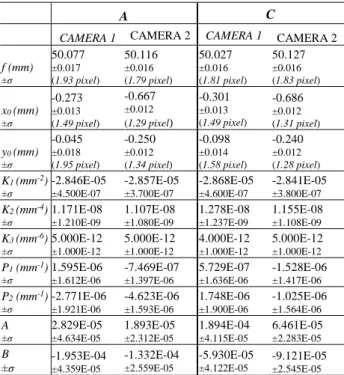
The experiment A is a conventional calibration with bundle adjustment, with no constraints in the RO between cameras. In experiment C several constraints were imposed, including the measured distance between perspective centers. In Figure 6.c the a posteriori variances for all the 4 experiments are presented. The increase in the a posteriori variance with the constraints is noticeable, and it is higher as the constraints have higher weight. Table 2 presents the estimated IOP and their estimated standard deviations for the 2 cameras used, in experiments A and C. The units for the focal length and principal point coordinates are mm and pixels, respectively.

A C

CAMERA 1 CAMERA 2 CAMERA 1 CAMERA 2

f (mm) ±σ 50.077 ±0.017 (1.93 pixel) 50.116 ±0.016 (1.79 pixel) 50.027 ±0.016 (1.81 pixel) 50.127 ±0.016 (1.83 pixel) x0 (mm) ±σ -0.273 ±0.013 (1.49 pixel) -0.667 ±0.012 (1.29 pixel) -0.301 ±0.013 (1.49 pixel) -0.686 ±0.012 (1.31 pixel) y0 (mm) ±σ -0.045 ±0.018 (1.95 pixel) -0.250 ±0.012 (1.34 pixel) -0.098 ±0.014 (1.58 pixel) -0.240 ±0.012 (1.28 pixel) K1 (mm-2) ±σ -2.846E-05 ±4.500E-07 -2.857E-05 ±3.700E-07 -2.868E-05 ±4.600E-07 -2.841E-05 ±3.800E-07 K2 (mm-4) ±σ 1.171E-08 ±1.210E-09 1.107E-08 ±1.080E-09 1.278E-08 ±1.237E-09 1.155E-08 ±1.108E-09 K3 (mm-6) ±σ 5.000E-12 ±1.000E-12 5.000E-12 ±1.000E-12 4.000E-12 ±1.000E-12 5.000E-12 ±1.000E-12 P1 (mm-1) ±σ 1.595E-06 ±1.612E-06 -7.469E-07 ±1.397E-06 5.729E-07 ±1.636E-06 -1.528E-06 ±1.417E-06 P2 (mm-1) ±σ -2.771E-06 ±1.921E-06 -4.623E-06 ±1.593E-06 1.748E-06 ±1.900E-06 -1.025E-06 ±1.564E-06 A ±σ 2.829E-05 ±4.634E-05 1.893E-05 ±2.312E-05 1.894E-04 ±4.115E-05 6.461E-05 ±2.283E-05 B ±σ -1.953E-04 ±4.359E-05 -1.332E-04 ±2.559E-05 -5.930E-05 ±4.122E-05 -9.121E-05 ±2.545E-05

Table 2. Estimated IOP and their estimated standard deviations for the two cameras, in experiments A and C.

Analyzing Table 2 it can be noted that the estimated standard deviations of parameters did not presented remarkable differences for the experiments A and C for both cameras, except by the standard deviation of the parameter y0 for camera 1, that reduced 0.37 pixels from experiment A to C. It was also noted that the estimated standard deviations of parameters f, x0 and y0 were slightly higher in experiment D. Due to lack of space details of these experiments are omitted in this paper.

The discrepancies between IOPs of cameras 1 and 2, respectively, estimated in experiments B, C and D, with respect to IOPs estimated in the experiment A, were computed. Analyzing theses discrepancies, it can be seen that the discrepancies are almost similar from experiments B and C. Experiment D, however, exhibits a different pattern, with some parameters presenting discrepancies with different sense (f,y0 and A, camera 1; K1and A of camera 2). In these experiments (D) the weight applied to the constraints can be considered high, because the variations admitted in the rotations are 1”. This means that the weight to be used have to be compatible with the uncertainty in the determination of EOP, otherwise these constraints will affect the estimated IOP.

In order to assess the influence of RO constraints in the EOP the standard deviation for the experiments A and C are shown in Figure 5. After parameters estimation, the Relative Orientation elements (angles Κ, Φ and Ω and base distance) can be computed from the EOP of each image. Table 3 presents the average values and standard deviations of these elements.

Ω Φ Κ Base distance A Average -36º 42' 55'' -0º 23' 18'' 179º 3' 50'' 10.452 cm ±σ ±0º 1' 54'' ±0º 1' 44'' ±0º 1' 7'' ±0.3478 cm B Average -36º 41' 53'' -0º 24' 54'' 179º 3' 14'' 11.103cm ±σ ±0º 1' 03'' ±0º 0' 11'' ±0º 0' 38'' ±0.0006cm C Average -36º 41' 33'' -0º 24' 50'' 179º 3' 15'' 11.120 cm ±σ ±0º 0' 52'' ±0º 0' 9'' ±0º 0' 37'' ±0.0007 cm D Average -36º 45' 53'' -0º 26' 17'' 179º 3' 17'' 9.556cm ±σ ±0º 0' 00'' ±0º 0' 00' ±0º 0' 00'' ±0.0023cm

Table 3. Average values and standard deviations of RO elements, computed from EOP, for each experiment.

Table 3 shows that the RO elements were estimated accordingly with the imposed constraints and the admitted variations. Analyzing Table 3 it can be noted that there are variations rounding 1’ to 2’ for the RO rotations and 3.4 mm for the base distance. These values are, of course, due to the uncertainties in the indirect estimation processes instead of physical variations itself. Introduction of RO constraints remedies this problem, as one can se in Table 3 (experiments B, C and D). Imposing RO constraints leads to more consistent solution both for RO rotations and base distance. A noticeable result achieved in the experiment B is related to the base distance. The average value computed from EOPs is 111.03mm, while the value measured directly is 111.2mm (a discrepancy of 0.17mm). Considering the uncertainness in the direct measurement, it is reasonable to state that the value estimated indirectly, by bundle adjustment, is consistent with the direct measurement, and the estimates can

(a)

(b)

Figure 5 - Estimated standard deviations of the parameters k, φ, ω, X0, Y0and Z0 in the experiments: (a) A (without RO constraints) and; (b) C (with RO constraints).

be considered accurate. Due to this accuracy, the introduction of the distance directly measured, as an additional constraint did not improve significantly the results, as one can se in Table 3 (experiment C).

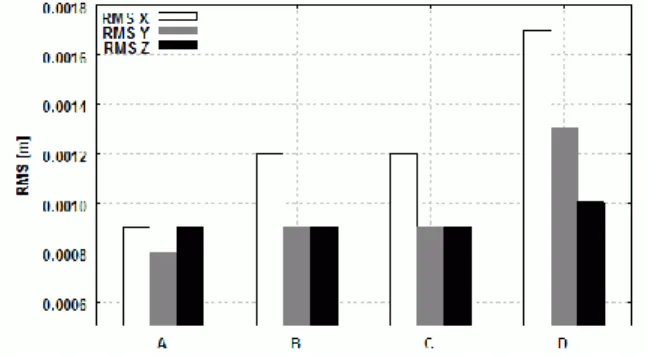
Figure 6 shows the RMS of the discrepancies between the field coordinates of check points and its estimated values by bundle adjustment for the four experiments.

Figure 6. RMS of the discrepancies between the field coordinates of check points and its estimated values.

The analysis of Figure 6 shows that the discrepancies in the object space coordinates increase proportionally with weights in the constraints imposed to the RO elements. This increase is probably due to error propagation from estimated EOP and IOP to the object space. The RMSE of the discrepancies are similar in Experiments A to C. However, in the experiment D there is a noticeable increase in the discrepancies in the coordinates of check points. The RMSE in the coordinate X in almost twice in the experiment D when compared to experiment A. These experiments showed that it is crucial to balance the values to impose to the RO constraints.

From the analysis of experiments carried out with the existing dual-head SAAPI system some conclusions can be given:

 In general, the RO constraints have to be imposed with a suitable weight. From our experiments, 30” for the rotations and 1mm for the distance are reasonable assumptions. The weight to be used in the pseudo-observations have to be estimated by covariance propagation, since the angular elements of RO are not considered as parameters in this approach;

 Imposing RO constraints with high weights reflects negatively in the results: the residuals in the observations are higher as well as the discrepancies in the check point coordinates;

 The estimated standard deviations of the EOP with RO constraints are slightly lower; however, the discrepancies in some check points, mainly in the peripheral are of the test field are higher with the bundle adjustment with RO constraints.

5. CONCLUSIONS

In this paper a method for dual-head camera calibration based on bundle adjustment was presented and experimentally assessed. The method proposes the imposition of Relative Orientation constraints, which states that orientation between cameras and distance between perspective centers can vary within certain values. The variations to be admitted were experimentally assessed and it was noted that imposing constraints with higher weights could lead to inaccurate results. The variations in the RO elements can be credited to physical

variations due to vibrations, temperature or mechanical locking, or even to the uncertainty in the estimation of the EOP parameters, to which RO elements are functionally related.

Experimental work with higher dimensions test field, providing ideal geometric conditions would be recommended. The same approach can be used for multi-head camera calibration, which experimental evaluation is left as a suggestion for future work. Also, the assessment of these results with aerial images is a topic for further research.

6. REFERENCES

Brown, D. C., 1966. Decentering distortion of lenses. Photogrammetric Engineering, 32(3), pp. 444-462.

Brown, D., 1971. Close-Range Camera Calibration, Photogrammetric Engineering, 37(8), p. 855-866.

Clarke, T. A., Fryer, J. G., 1998. The development of camera calibration methods and models. Photogrammetric Record, 16(91), pp. 51-66.

Cramer, M., 2004. EuroSDR network on digital camera calibration. Institute of photogrammetry, University of Stuttgart, Final Report, oct. 2004. Disponível em: <http://www.ifp.uni-stuttgart.de/eurosdr/EuroSDR-Phase1-Report.pdf>. 02 jul. 2007. Doerstel, C.; Zeitler, W.; Jacobsen,K.,2002.Geometric calibration of the DMC: method and results. In: The International Archives for Photogrammetry and Remote Sensing, 34(1), Denver, USA, pp 324 – 333,.

Habib, A.; Morgan, M., 2003. Automatic calibration of low-cost digital cameras. Optical Engineering, 42(4), pp. 948-955.

Merchant, D. C., 1979. Analytical photogrammetry: theory and practice. Notes Revised from Earlier Edition Printed in 1973, The Ohio State University, Ohio State. .

Mikhail, E. M.; Ackerman, F., 1976. Observations and least squares. New York: A Dun-Donnelley Publisher.

Mikhail, E. M.; Bethel, J. S.; Mcglone, J. C., 2001. Introduction to modern photogrammetry. New York: John Wiley & Sons, 2001. Moniwa, H., 1972 Analytical camera calibration for close-range photogrammetry. Thesis, New Brunswick, Master of Science, University of New Brunswick.

Roig, J.; Wis, M.; Colomina, I., 2006. On the geometric potential of the NMC digital camera. In: Proceedings of the International Calibration and Orientation Workshop – EuroCOW 2006, 25-27 January, Castelldefels, Spain.

Ruy, R. S.; Tommaselli, A. G.; Hasegawa, J. K.; Galo, M.; Imai, N. N.; Camargo, P. O., 2007. SAAPI: a lightweight airborne image acquisition system: design and preliminary tests. In: Proceedings of the 7th Geomatic Week – High resolution sensors and their applications, Barcelona, Spain.

Zhuang, H., 1995. A self-calibration approach to extrinsic parameter estimation of stereo cameras.Robotics and Autonomous Systems, 15, pp. 189-197.

Mostafa, M. M. R.; Schwarz, K. P., 2000. A Multi-Sensor System for Airborne Image Capture and Georeferencing. Photogrammetric Engineering & Remote Sensing, 66(12), pp. 1417-1423.

7. ACKNOWLEDGEMENTS

The authors would like to acknowledge the support of CNPQ (Conselho Nacional de Desenvolvimento Cientifico e Tecnológico), with a Master Scholarship and a Research Grants (472322/04-4 and 481047/2004-2). The authors are also thankful to FAPESP (Fundação de Amparo à Pesquisa do Estado de São Paulo) and to Engemap Geoinformação for providing the resources for image acquisition.