Teaching on Jupyter - Using notebooks to
accelerate learning and curriculum development
Reades, Jonathan
Veröffentlichungsversion / Published Version Zeitschriftenartikel / journal article
Empfohlene Zitierung / Suggested Citation:
Reades, J. (2020). Teaching on Jupyter - Using notebooks to accelerate learning and curriculum development. Region: the journal of ERSA, 7(1), 21-34. https://doi.org/10.18335/region.v7i1.282
Nutzungsbedingungen:
Dieser Text wird unter einer CC BY-NC Lizenz (Namensnennung-Nicht-kommerziell) zur Verfügung gestellt. Nähere Auskünfte zu den CC-Lizenzen finden Sie hier:
https://creativecommons.org/licenses/by-nc/4.0/deed.de
Terms of use:
This document is made available under a CC BY-NC Licence (Attribution-NonCommercial). For more Information see: https://creativecommons.org/licenses/by-nc/4.0
Teaching on Jupyter – Using notebooks to accelerate
learning and curriculum development
Jonathan Reades1
1King’s College London, London, United Kingdom
Received: 7 October 2019/Accepted: 5 January 2020
Abstract. The proliferation of large, complex spatial data sets presents challenges to the way that regional science and geography more widely is researched and taught. Increasingly, it is not ‘just’ quantitative skills that are needed, but computational ones. However, the majority of undergraduate programmes have yet to offer much more than a one off ‘GIS programming’ class since such courses are seen as challenging not only for students to take, but for staff to deliver. Using the evaluation criterion of minimal complexity, maximal flexibility, interactivity, utility, and maintainability, we show how the technical features of Jupyter notebooks particularly when combined with the popularity of Anaconda Python and Docker enabled us to develop and deliver a suite of three ‘geocomputation’ modules to Geography undergraduates, with some progressing to data
science and analytics roles.
1 Introduction
The growth of data from sources that are both ‘accidental, open, and everywhere’ (Arribas Bel 2014), and characterised by volume, velocity, variety, and questions of veracity (Gorman 2013) has opened up new possibilities, and challenges, for researchers. This, in turn, calls for new conceptual, methodological, and technical approaches since ‘acquiring data is no longer a strongly limiting factor to completing analytical tasks’ (Bowlick, Wright 2018), working with it is. It is not particularly important whether these skills are framed as an informed empirical social science (Ruppert 2013) or as a computational social science (Lazer et al. 2009); authoritative reviews of the social sciences and humanities byThe British Academy(2012), and of human geography by the Economic and Social Research Council (Ley et al. 2013), have concluded that many graduates are poorly prepared to engage with this world of ‘big data’. The Royal Society(2019) has called for curriculum change at Higher Education Institutions (HEIs) with a view to encouraging interdisciplinarity and the effective integration of data science skills.
This presents something of a problem for a nascent ‘geographic data science’ (Singleton, Arribas Bel 2019) of the sort that regional science, and regional studies and geography more widely, require since a surprisingly large number of university programmes continue to teach proprietary, mostly point-and-click software. So many students’ principal exposure to quantitative methods, let alone computational ones, comes in a standalone ‘quantitative methods module’ that provides little in the way of meaningful interaction with the underlying issues of spatial data and spatial data analysis at scale. And while the issue may be particularly acute for students in the U.K. (Johnston et al. 2014), even in more technically-oriented countries there is often not much more on offer than a
straightforward ‘GIS course’ (Wikle, Fagin 2014). Consequently, students progressing to higher levels of study or the professional realm often find that ‘the skills least developed in undergraduate GIS courses are those related to programming and computer science’ (Bowlick et al. 2017).
2 Dependencies
This notebook requires theGeoJSON labextension to be installed in JupyterLab. All other packages should be part of a default Python 3 installation.
3 Context
The long history of computers in geography has not been without controversy (Arribas Bel, Reades 2018,Barnes 2013,Cresswell 2014,Johnston et al. 2014), although many have actively engaged with recent developments (e.g.Torrens 2010) and expect impacts on the very fabric of the discipline (Gonz´alez Bail´on 2013). So although our experience with teaching computational skills using Jupyter notebooks is clearly rooted in the ‘geography of geography’ (Bradbeer 1999) in the sense that we speak to particular challenges here in the U.K., it is part and parcel of a wider skills gap at the undergraduate level in general. In short, too few students are gaining the skills needed to engage with this deluge of data or to take advantage of cutting-edge tools developed outside of the field, either as researchers or as end-users in the public or private sectors (Singleton 2014).
This is where we believe that the pedagogical potential ofProject Jupyter(Kluyver et al. 2016) is revolutionary: reflecting on our experience of trying to roll out exactly this type of programme, we seek to highlight the transformative potential of notebooks for student and researcher development. Jupyter removes significant barriers to teaching by providing a flexible and familiar interface that hides, or even postpones indefinitely, some of the complexity of managing local programming language installations whilst also allowing instructors to provide rich media and contextual information next to the code where it is needed the most. Making coding accessible is not simply about allowing students to ‘hack away’ at data, it can actuallyhelp students to better understand spatial analytic methods by linking concepts to code as Xiao’s outstanding text on algorithms demonstrates (Xiao 2016).
3.1 Teaching Programming to Non Programmers
Given the interaction effects between pedagogical and subsequent practice, it is therefore worth placing the challenge of teaching programming in the context of the shifting terrain for quantitative research and researcher development. These challenges start early: many students already demonstrate whatSpronken-Smith(2013) calls ‘equation phobia’: “students not linking numbers, and problems with visualisation of quantities.” Hodgen et al.(2014) suggest just some of the reasons for this: limited prior knowledge and attainment; time elapsed since last study of maths; a failure to see relevance; and the wide range of attainment levels within each cohort (Hodgen et al. 2014). Whatever its origins, a general lack of confidence and/or competence creates a feedback loop fuelling further avoidance (Chapman 2010).
In the context of maths instructionMacdonald, Bailey (2000) have also noted the challenge inherent in delayed gratification given that ‘maths is the tool, not the goal.’ Given the apparent gulf betweenprint('Hello world.')and being able to write useful analytical code, the issue is no less serious in programming. There is no reason why the familiarity of so-called ‘Digital Natives’ with computers should have any bearing on their understanding of how they actually work; indeed, today’s students may well be more detached from the underlying processes – metaphorical and actual – thanks to ‘the sophistication of modern Graphical User Interfaces’ (Muller, Kidd 2014). In the long run, programming requires an ability to envision and manipulate abstract entities such as data structures sitting, in turn, on top of additional layers of abstraction such as the application and its state(s), the file system and its structure(s), the operating system and even the underlying hardware.
Figure 1: Barron Stone memorably demonstratesfor andwhile loops (Stone 2013)
There are many differing views of how programming should be taught (Pears et al. 2007), though we come down firmly on the side ofLukkarinen, Sorva(2016) that there are advantages to ‘contextualising programming practice in the field of application’. In general, it seems that introductory programming courses should strive simultaneously for richness and simplicity: richness in the ‘constructs’ associated with programming, and simplicity in terms of the foundation being laid (Lukkarinen, Sorva 2016). Unfortunately, the expertise of teachers is not always a plus for effective teaching (Chapman 2010) since concepts that seem intuitive and are easily connected to a range of related problems by the instructor may yield no such benefit to the novice. As we developed our teaching materials, we found that videos created by other learners could, at times, capture student attention more effectively than our own demonstrations; for example, Stone’s instructional video for students at Rice University on the difference between for and while loops, shown in Figure1. Using Jupyter notebooks this kind of content can be embedded directly in the task explanation.
3.2 Course Structure
The work reported here draws on methodological and pedagogical research conducted over the past five years in theDepartment of Geography atKing’s College London; it seeks both to position learning to code as essential to further student and staff development, and to examine the reasons why Jupyter notebooks have been selected as the best means of achieving this goal. As such, this research is necessarily caught up in a wider debate about quantitative skills amongst students; however, our undergraduate ‘pathway’ in Geocomputation & Spatial Analysis(which could be understood as an optional ‘minor’ in the North American tradition) seeks to go beyond the kinds of statistical skills training encouraged by funders (see brief discussion in Johnston et al. 2014) and to tackle these in conjunction with computational skills. We want to take students with a variety of social, economic, ethnic, and computational backgrounds and cultivate in (and with) them an appreciation of, and ability to undertake, interdisciplinary work with a strong computational element (seeMir et al. 2017, for a discussion of theCS+X format).
Based on our own experience, we felt that shoe horning exposure to ‘computational geography’ into a single module – as seems to occur in many American programmes (Bowlick et al. 2017) – would only reinforce student aversion to such approaches, so we opted to ‘unpack’ the concepts across three modules:
1. Geocomputation
2. Spatial Analysis and Modelling, and 3. Applied Geocomputation.
These modules must be taken in sequence, the preceding module acting as a pre-requisite for admission to the next, although students are free to exit the sequence at any time. We also provide an optional ‘Code Camp’ (Reades et al. 2019) to be undertaken over the summer before the first module begins so that students begin the term familiar with basic concepts: variables, lists/arrays, dictionaries/hashes, and functions/subroutines, provided they have done the work.
3.3 Contextualised Computing
To our knowledge, there is no other undergraduate programme like it with important differences in both style and substance from what would be covered in an Economics, Statistics, or Computer Science (CS) degree in terms of its spatial and applied focus. In this sense, the modules are an extended test of ‘contextualised computing’ instruction (see Lukkarinen, Sorva 2016, for a review) which seeks to emphasise relevance to ‘real-world’ applications and to avoid “general CS content, such as how one might go about sorting an array of any type for an unspecified purpose” (Lukkarinen, Sorva 2016). We also recognise, however, that “contextualized computing education cannot help students learn more in less time” (Guzdial 2010) and that thetransferrable aspects of this learning need to be emphasised: in our case we try to highlight how the same approach can be applied to human and physical geography problems.
Consequently, wherever possible these exercises are grounded in spatial examples, even where these are very simple indeed, on the basis that connecting them to the learner’s existing knowledge and interests will improve retention at the introductory level (Guzdial 2010). For example, a notebook on dictionaries (taken from Reades et al. 2019) can start with creating and querying a phone book of national emergency numbers where the student has to replace the???ineNumbers = { ??? }with functioning Python code: [1]: eNumbers = {
'IS': 112, 'US': 911 }
print(f"The Icelandic emergency number is {eNumbers['IS']}") print(f"The American emergency number is {eNumbers['US']}")
[1]: The Icelandic emergency number is 112 The American emergency number is 911
Students then progress towards a task involving a dictionary-of-dictionaries: [2]: cityData = { 'London': { 'population': 8673713, 'location': [51.507222, -0.1275], 'country': 'UK' }, 'Paris': { 'population': 2140526, 'location': [48.8567, 2.3508], 'country': 'FR' } }
for city, data in cityData.items():
print(f"The population of {city} ({data['location'][0]:0.3f}ºN, {data['location'][1]:0.3f}ºE) is {data['population']:,}")
[2]: The population of London (51.507ºN, 0.128ºE) is 8,673,713 The population of Paris (48.857ºN, 2.351ºE) is 2,140,526
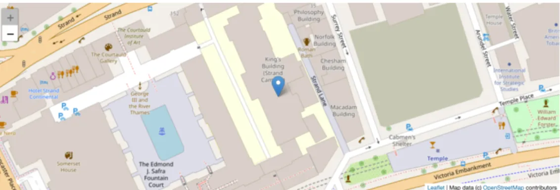
This work is building towards a GeoJSON example in which they have to complete missing attributes in order to show a marker centred on the university’s central London campus. Since GeoJSON is essentially a dictionary-of-dictionaries, this is a good test of their understanding, but with Jupyter they receive immediate feedback on this because GeoJSON can be embedded directly into the notebook: an interactive web map shows up
as soon as they’ve run the code, reinforcing the contextual aspect – that this isall about geography – of their learning.
[3]: # King’s College London’s coordinates...
# What format are they in? Does it seem appropriate? # How would you convert them back to numbers if you # needed to do so?
longitude = '-0.11596798896789551' latitude = '51.51130657591914'
# Notice how we set up a data type and location # here where it’s easy to see where the lat/long # values are being used we could also use these # in a loop as a _template_ for creating many points # from a data file! Notice too that it’s a dictionary # containing a mix of string and list values... the_geometry = {
"type": "Point",
"coordinates": [longitude, latitude], }
# Now we set up the larger ’data file’ this is harder # to read but is *still* basically a dictionary! A # ’collection’ implies more than one feature, and in this # case the list of ’features’ is nothing more than a list # of dictionaries so that our data stays in order! the_position = { "type": "FeatureCollection", "features": [ { "type": "Feature", "properties": { "marker-color": "\#7e7e7e", "marker-size": "medium", "marker-symbol": "building", "name": "KCL" }, "geometry": the_geometry } ] }
# And show the points on an interactive map!
# You don’t need to know what’s happening here *yet*, but # see if you can make sense of the main elements... try:
from IPython.display import GeoJSON from IPython.display import display import json
parsed = json.loads(str(the_position).replace("\'", "\"")) display(GeoJSON(parsed))
except ImportError:
print("You seem to be missing either the GeoJSON extension or json library.")
[3]: The output is shown in Figure 2
4 How We Reached Jupyter
Since the pathway pushes students both conceptually and technically, finding ways to take the deployment and management of the software stack out of the picture has been a priority. Our review of the pedagogical literature and practical experience gained in the private and HEI sectors—including several failures during the first few years of teaching—led us to the ultimate conclusion that a useful geospatial programming environment should possess the following characteristics:
Minimal Complexity : it does not require students to load and learn a new Operating System or large number of new applications/platforms at the same time as they are
Figure 2: Output of code 3
learning to code; it should also be reasonably ‘performant’ on a mix of student and HEI hardware.
Maximal Flexibility : it is simple, if not always easy, to configure and install on a range of hardware, but is not ‘sandboxed’ or ‘packaged’ in ways that constrain our freedom to install what we need to teach effectively.
Interactivity : it allows us to keep commentary, ‘rich’ media, and other scaffolding material together with the code so that students can move between code and explanations easily, and can add their own annotations as needed.
Utility : it supports life-long learning by providing a ‘real world’ development environ-ment that would be both familiar, and accessible, to students after graduation in personal and professional contexts.
Maintainability : it can be easily updated by the instructor(s) and supports version control and easy distribution mechanisms.
These five features can, at times, appear to cut against each other: maximal flexibility and minimal complexity are difficult to reconcile since the former tends to expose more ‘options’ to the user, while the latter seeks to mask those same options. However, a strong advantage of Jupyter is that it meets all of these criteria to some extent, and in most cases meets them fully!
4.1 Pretty Walled Gardens
The desired set of features ruled out commonly-used proprietary platforms: at the time we began developing the curriculum, MATLAB was still ade factostandard for many but its pricing and sandboxing approach made it both less flexible and less useful for students once they graduated and lost access to the HEI license. LikeEtherington(2016), we were therefore attracted by the fact that Python presented ‘no financial or hardware obstacles to teaching’ and that, consequently, “students [would] always be able to use their Python programming skills...”Etherington (2016). However, in developing the early iterations of the course we also, again like Etherington(2016), encountered significant challenges in ‘getting a working installation of Python together with its associated geospatial packages’.
We discovered that the existing, IT-supported Enthought Canopy Python distribution provided few of geospatial libraries, and that updating it with packages from outside of their ‘walled garden’ caused all manner of issues. This situation was not entirely unexpected since geospatial analysis is not a key component of Enthought’s offering to universities; however, the challenges of keeping up with the state-of-the-art are such that additional barriers to software update management are undesirable. Indeed, the pace of change in the field can be gauged from Wise’s review of ‘geospatial technologies’ in U.K. universities (Wise 2018): it not only questions the utility of ‘free’ programmes (presumably meaning Free Open Source Software, or FOSS) which now dominate in the data sciences and in many research projects, but it also contains not a single mention of programming—in Python or any other language.
4.2 The Wrong Kind of Flexibility
LikeMuller, Kidd(2014), who sought to ‘debug geographers’ with an introduction to a holistic computing context alongside programming skillstout court, we next attempted to provide our students with virtualised Linux desktop systems in the belief that this would empower them not only with a better understanding of what was going on ‘under the hood’ but also with a computer on which they could experiment without fear of damaging their existing installation. For good measure, we included other useful analytics tools such as the latest version of QGIS with all of the ‘bindings’ for low-level packages such as GDAL (the Geospatial Data Abstraction Layer).
Using VMWare and Ubuntu 16 LTS with a full Python installation configured largely ‘by hand’ provided us with a fully FOSS ‘solution’ that students could take with them and update in the future as they gained confidence in using such software. However, we soon found that in-memory and on-disk bottlenecks, together with students’ tendency to actually try to install Ubuntu’s suggested updates and render their systems inoperable, made this a profoundly alienating and frustrating experience. For students already working hard to master the basics of programming, having to ‘drop’ into the Terminal in order to resolve installation errors when they were used to seamless updates on their host operating systems simply represented an unnecessary hassle that detracted from the real focus of the modules: learning to use code to perform spatial analyses.
4.3 Escape Velocity
While we had been tinkering with different Linux and Python distributions, a set of three connected developments had been transforming the landscape for teaching:
1. A few academics who had taken very different approaches began, rather bravely, to publish their teaching methods and materials freely for others to use (e.g.Arribas Bel 2019);
2. Data scientists not only adopted Pythonen masse, driving the rapid development of new analytical and visualisation libraries (e.g. pandas, seaborn, bokeh), but they had also quickly settled on the use of a then-novel technology called ‘iPython notebooks’ to widely share their tutorials online;
3. Since many of these data scientists were paid by firms interested in moving their work into production systems as smoothly and quickly as possible, this also led to improvements in the way that Python distributions and notebooks were managed. Rather unexpectedly, the kinds of practical problems that data scientists were trying to solve mirrored quite closely the kinds of challenges that we, as teachers, were trying to solve in terms of being able to replicate installations across multiple systems and share code/commentary quickly and easily.
The iPython platform ultimately gained the ability to run other programming lan-guages and was rebranded ‘Project Jupyter’, but this means that it has become a viable, general purpose teaching platform. So although the term ‘Virtual Learning Environment’ (VLE) is typically understood to refer to a full-featured, client-server system such as Moodle or Blackboard (seeBritain 1999), it could also apply to Jupyter: not only does it have a client/server architecture (with the web-based interface allowing the server to run locally or on a remote system with no discernible difference to the student), but it has been progressively enriched with tools for grading and other common teaching tasks. Although we are not yet making full use of these new features, it is clear that Jupyter is well on its way to becoming an important teaching platform.
5 Discussion
Perhaps the single greatest benefit of working with Jupyter notebooks is that development isnot being driven by educational needs: this is a full-featured development environment used day-in and day-out by professional software developers and large firms such as Netflix
(Ufford et al. 2018). So, unlike both expensive proprietary systems that are rarely used by small or innovative firms, and instructional systems whose functionality is limited to teaching purposes, students are able to seamlessly progress from learning to code, to competent coders, and on to practicing data scientists (as a few of our students have done), using a single environment. This is a platform with the capacity to grow with the student, following them out of the ‘ivory tower’ and into gainful employment.
An additional benefit flowing from the professional use of Jupyter is that many researchers, not least the others included in this special issue, use notebooks as a normal part of their research practice; this allows lecturers to remain abreast of technical developments on the platform without ‘updating my installation’ being a separate overhead in a congested working week. This pattern of usage is in sharp contrast to tools – such as SPSS or ArcGIS – that are less-used by active researchers but often still taught in standalone modules, with the quality and timeliness of teaching materials often suffering accordingly. Jupyter breaches the historical divide between computational research and teaching, not only allowing students to benefit from active research, but also for research to build on student outputs (see, for example Reades et al. 2019).
5.1 Cloning Around
Jupyter becomes particularly powerful when combined with other recent developments in the management and distribution of computing platforms. Anaconda Python’s enhanced support for the configuration of virtual environments (in essence, multiple distributions of Python on the same system) allows specific versions of Python and sets of required libraries to be specified in a simple text file following the ‘Yet Another Markup Language’ (YAML) standard. The code below downloads and prints out part of the YAML file that we use to configure both student machinesand our Docker container (about which more below); here the virtual environment is namedgsa2019:
[4]: import urllib
url = 'https://raw.githubusercontent.com/kingsgeocomp/gsa_env/gsa2019/gsa.yml' with urllib.request.urlopen(url) as resp:
file = resp.read().decode('utf8').split('\n') # Don’t output everything...
to_print = list(range(0,5)) list(range(39,48)) list(range(110,116))
print("=" * 50) for line in to_print: print(file[line]) print("=" * 50)
[4]: ==================================================
# OVERVIEW
# This YAML script will attempt to install a Python virtual environment able to # support the requirements of all three of King’s College London’s ’Geocomputation’ # pathway in the BA/BSc Geography programme.
# # CONFIGURATION PARAMETERS name: gsa2019 channels: - conda-forge - defaults dependencies: - python=3.7 - pip - git - xlrd - xlsxwriter - pip: - six
#- git\+http://github.com/sevamoo/SOMPY#egg=sompy # Doesn’t run in Python3 - git\+http://github.com/kingsgeocomp/SOMPY#egg=sompy
==================================================
Python and to expose this as a named ‘iPython kernel’. The connection between virtual environments and kernels allows researchers to manage multiple research and teaching installations of Python on the samesystem, to access them through the same Jupyter interface, and to do so without changes to one Python installation impacting any others. 5.2 Docking Safely
The emergence of containerisation platforms such asDockernow makes it much simpler to distribute a pre-configured virtual machine1(such as a pre-packaged teaching or research
environment) that will run on almost any host operating system: Mac, Windows, or Linux. Because the virtual machines are fully specified at the time of creation, students can download and install a working version with one command, while instructors can be confident that every student is working with thesame version of every library. This year we provided students with a Docker image that leveraged the work ofArribas Bel(2019) but that had been customised to provide only the features that we wished to teach.
The combined popularity of Python and Docker has led to the creation of novel, web-based platforms such as Binder (mybinder.org); these take notebooks stored on the GitHubcode-sharing web site to build a Docker image serving those notebooks on Binder’s servers. Students may now learn to code without installing any software whatsoever. Local installation can be deferred to the point at which specialist requirements or load on the server require it. In a stroke, one of the most pernicious barriers to entry, needless technical issues associated with installation and configuration of programming software, has been eliminated.
5.3 Houston, We Have a Problem
Of course, no single solution is without drawbacks and Jupyter is no exception. It is worth noting that there are quite specific technical, conceptual, and development issues raised by Jupyter that are difficult to circumvent without both know-how and some careful thinking about assessment and teaching. The principal technical challenge relates to user permissions on managed machines (e.g. in computer clusters) since Python, Jupyter, and Docker all struggle to different degrees with ‘locked down’ Windows systems. Indeed, Docker does not currently run at all without administrator privileges. We worked closely with university-level IT staff to install and provision Anaconda Python and Jupyter. Provision of the YAML configuration scriptassisted with both installation and isolation of our teaching environment from their existing installation, easing institutional barriers to adoption.
From a teaching standpoint, an additional issue is thatGit– the dominant version control software that we use to manage and share notebook changes – sees notebooks in a way that means just re-running code registers as a local modification of the file that needs to be committed to the version control system. So although ‘GitHub’ provides support for the online display of Jupyter notebooks, the use of Git can lead to a large number of essentially meaningless commits. This can make tracking meaningful content changes over time more difficult, and it means that we’ve shied away from teaching students about version control on the basis that they may not perceive the value of commits that seem to record little of value.
A final and rather unexpected disbenefit was uncovered the year after we moved from the Spyder IDE to Jupyter: weaker student understanding of execution flow. Unlike a traditional script that clearly executes from top-to-bottom (typically in its entirety), Jupyter notebooks freely intermingle code blocks and text/rich media blocks allowing – and even encouraging – the user both to jump between widely separated blocks without executing intervening code and to edit and re-run earlier blocks. This leads to: a) difficult-to-diagnose bugs because the codelooks like it should execute properly but doesn’t, and b) to a weaker student understanding of system ‘state’ in terms of instantiated variables, loaded libraries, and available functions. We typically seek to cultivate this understanding by stressing that thereal test, whether directly assessed or not, of whether their code
1It should be noted that, technically, Docker containers are not virtual machines in the traditional sense.
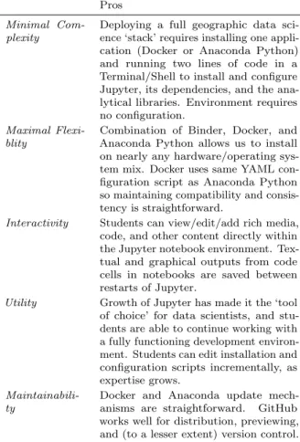
Table 1: Evaluating Jupyter
Pros Cons
Minimal Com-plexity
Deploying a full geographic data sci-ence ‘stack’ requires installing one appli-cation (Docker or Anaconda Python) and running two lines of code in a Terminal/Shell to install and configure Jupyter, its dependencies, and the ana-lytical libraries. Environment requires no configuration.
Persistent challenges with student un-derstanding of file system interaction and paths. Some confusion around mul-tiple Python instances manifesting as different ‘kernels’ in notebooks.
Maximal Flexi-blity
Combination of Binder, Docker, and Anaconda Python allows us to install on nearly any hardware/operating sys-tem mix. Docker uses same YAML con-figuration script as Anaconda Python so maintaining compatibility and consis-tency is straightforward.
Students cannot update Docker con-tainers and do not gain understanding of package management or dependency conflict resolution.
Interactivity Students can view/edit/add rich media, code, and other content directly within the Jupyter notebook environment. Tex-tual and graphical outputs from code cells in notebooks are saved between restarts of Jupyter.
Students do not develop a strong under-standing of execution flow and system state.
Utility Growth of Jupyter has made it the ‘tool
of choice’ for data scientists, and stu-dents are able to continue working with a fully functioning development environ-ment. Students can edit installation and configuration scripts incrementally, as expertise grows.
Relative ease of installation may not pre-pare students for managing their own de-velopment and production environments. Students remain unfamiliar with IDEs and code-completion.
Maintainabili-ty
Docker and Anaconda update mech-anisms are straightforward. GitHub works well for distribution, previewing, and (to a lesser extent) version control.
Nature of notebooks makes it harder for instructors to track incremental changes in version control, and for students to see value of such an approach.
‘works’ is that a notebook can be run in full (Restart Kernel and Run All Cells) without user intervention.
We should note that, in the absence of an Integrated Development Environment (IDE), students are unlikely to benefit from test suites and other tools that support developer best-practice. However, such an approach can also have the effect of deterring new students by pushing back the point at which they appear to be achieving anything concrete: “Because learning in computer science and programming is challenged by numerous barriers, students need to be motivated about the purpose, value, and utility of concepts within course work” (Bowlick et al. 2017) So while knowledge of professional tools and practices is desirable, we nonetheless feel that these kinds of ideas and issues are best tackled when students have progressed further with their studies and are motivated to tackle more abstract challenges.
6 Conclusion: Back Here on Earth
In order to understand why the practical benefits of teaching with Jupyter notebooks outweigh the technical and conceptual challenges encountered, it is worth returning to the evaluation criteria outlined near the start of this work. Table 1summarises the pros and cons observed across the five dimensions identified by our review of the state-of-the-art nearly six years ago.
From this, the principal technical recommendation is that a flexible mix of platforms should be used to deliver Jupyter-based learning. We recommend Binder to deliver foundational material using few non-core Python libraries, and now strongly recommend that students use Docker in subsequent modules. However, a critical issue is that Windows 10 Home Edition does not support Docker, and it is thereforestill necessary to support direct installation ofAnaconda Pythonand associated configuration of the ‘kernel’ using a
YAML text file. We are also investigating the use of acontainerised JupyterHubrunning on our own hardware: this would allow students to mimic using Binder while benefiting from the ability to save work and make full use of Python’s capabilities. All of the code supporting these configurations is available as aGithub repository, as is Arribas-Bel’s resource.
6.1 And Back to the Future
A failure to engage directly with computational approaches and tools poses long-term risks: while ours ‘has always been a following discipline’ (Burton 1963), what is new is that other disciplines have now taken an interest in cities and regions (O’Sullivan, Manson 2015). Ruppert(2013) warns, “if social scientists do not step forward, then computational social science risks becoming the exclusive domain of . . .computing scientists” (Ruppert (2013). However, there is also an enormous opportunity for students equipped with both domain knowledge and programming skills to act as ‘knowledge brokers’ (Bowlick, Wright 2018). AsMir et al.(2017) note: “truly transformative work at the intersection of computing and. . . other disciplines requires. . .people with heterogeneous skill-sets (both computational and non-computational) who, despite their differences in training, can work collaboratively.” In other words, facing the future requires both translators and explorers: individuals who understand the broader terrains across which knowledge moves and the frontiers at which new knowledge is generated.
We have also come to believe that the use of Jupyter-like platforms in non-STEM disciplines may have a role to play in addressing a deeper problem: the widening par-ticipation challenge in computationally-oriented disciplines such as data science (The Royal Society 2019). A particular contribution is these other disciplines’ capacity to provide an applied context for computational training that helps to motivate further study and engagement (seeBort et al. 2015, for a creative application in literary studies). It should not be the responsibility of Geography and allied fields to plug the so-called ‘leaky pipeline’ (Berryman 1983), but they may yet create novel pathways for a more diverse cohort of students to enter computationally intensive fields. Such an outcome would not only be to the benefit of Computer Science, it would very much be to the benefit of an innovative Regional Science as well.
Acknowledgements
This work builds on the input of many – staff and students – to the Geocomputation and Spatial Analysis pathway at King’s College London; however, I wish to particularly acknowledge the critical contributions ofDr. James Millington,Michele Ferretti,Dr. Chen Zhong, andDr. Yijing Li. Finally,Dr. Arribas-Bel has donated many hours of his time – directly and by example – to helping me to develop and migrate our teaching environment.
References
Arribas Bel D (2014) Accidental, open and everywhere: Emerging data sources for the understanding of cities. Applied Geography 49: 45–53. CrossRef.
Arribas Bel D (2019) A course on geographic data science. The Journal of Open Source Education 2: 42. CrossRef.
Arribas Bel D, Reades J (2018) Geography and computers: Past, present, and future. Geography Compass e12403
Barnes T (2013) Big data, little history. Dialogues in Human Geography 3: 297–302 Berryman S (1983) Who will do science? Trends, and their causes in minority and female
representation among holders of advanced degrees in science and mathematics. A special report. Rockefeller Foundation, New York, NY
Bort H, Czarnik M, Brylow D (2015) Introducing computing concepts to non majors: A case study in gothic novels. Proceedings of the 46th ACM Technical Symposium on Computer Science Education, 132–137. ACM. CrossRef.
Bowlick F, Goldberg D, Bednarz S (2017) Computer science and programming courses in geography departments in the United States. The Professional Geographer 69: 138–150. CrossRef.
Bowlick F, Wright D (2018) Digital data centric geography: Implications for geography’s frontier. The Professional Geographer 70: 687–694. CrossRef.
Bradbeer J (1999) Barriers to interdisciplinarity: Disciplinary discourses and student learning. Journal of Geography in Higher Education 23: 381–396. CrossRef.
Britain S (1999) A framework for pedagogical evaluation of virtual learning environments. Report, Joint Information Systems Committee. https://www.webarchive.org.uk/way- back/archive/20140613220103/http://www.jisc.ac.uk/media/documents/program-mes/jtap/jtap-041.pdf
Burton I (1963) The quantitative revolution and theoretical geography. The Canadian Geographer/Le G´eographe Canadien 7: 151–162. CrossRef.
Chapman L (2010) Dealing with maths anxiety: How do you teach mathematics in a geography department? Journal of Geography in Higher Education 34: 205–213. CrossRef.
Cresswell T (2014) D´ej`a vu all over again: Spatial science, quantitative revolutions and the culture of numbers. Dialogues in Human Geography 4: 54–58
Etherington T (2016) Teaching introductory GIS programming to geographers using an open source python approach. Journal of Geography in Higher Education 40: 117–130. CrossRef.
Gonz´alez Bail´on S (2013) Big data and the fabric of human geography. Dialogues in Human Geography 3: 292–296. CrossRef.
Gorman S (2013) The danger of a big data episteme and the need to evolve geographic information systems. Dialogues in Human Geography 3: 285–291. CrossRef.
Guzdial M (2010) Does contextualized computing education help? ACM Inroads 1: 4–6. CrossRef.
Hodgen J, McAlinden M, Tomei A (2014) Mathematical transitions: A report on the mathematical and statistical needs of students undertaking undergraduate studies in various disciplines. Report, The Higher Education Academy
Johnston R, Harris R, Jones K, Manley D, Sabel C, Wang W (2014) Mutual misunder-standing and avoidance, misrepresentations and disciplinary politics: Spatial science and quantitative analysis in (United Kingdom) geographical curricula. Dialogues in Human Geography 4: 3–25. CrossRef.
Kluyver T, Ragan Kelley B, P´erez F, Granger B, Bussonnier M, Frederic J, Kelley K, Hamrick J, Grout J, Corlay S, Ivanov P, Avila D, Abdalla S, Willing C, Jupyter Development Team (2016) Jupyter notebooks – a publishing format for reproducible computational workflows. In: Loizides F, Schmidt B (eds), Positioning and power in academic publishing: Players, agents and agendas. IOS Press, 97–90
Lazer D, Pentland A, Adamic L, Aral S, Barab´asi A, Brewer D, Christakis N, Contractor N, Fowler J, Gutmann M, Jebara T, King G, Macy M, Roy D, Van Alstyne M (2009) Life in the network: The coming age of computational social science. Science 323: 721–723. CrossRef.
Ley D, Braun B, Domosh M, Elliott S, Le Heron R, Peake L, Willekens F, Yeoh B (2013) In-ternational benchmarking review of UK human geography. Report, Economic and Social Research Council, in partnership with the Royal Geographical Society (with IBG) and the Art and Humanities Research Council. https://esrc.ukri.org/files/research/research-and-impact-evaluation/international-benchmarking-review-of-uk-human-geography/ Lukkarinen A, Sorva J (2016) Classifying the tools of contextualized programming
education and forms of media computation. Proceedings of the 16th Koli Calling International Conference on Computing Education Research, 51–60. ACM. CrossRef. Macdonald R, Bailey C (2000) Integrating the teaching of quantitative skills across the geology curriculum in a department. Journal of Geoscience Education 48: 482–486. CrossRef.
Mir D, Mishra S, Ruvolo P, Pollock L, Engen S (2017) How do faculty partner while teaching interdisciplinary CS+X courses: Models and experiences.Journal of Computing Sciences in Colleges 32: 24–33
Muller C, Kidd C (2014) Debugging geographers: Teaching programming to non computer scientists. Journal of Geography in Higher Education 38: 175–192. CrossRef.
O’Sullivan D, Manson S (2015) Do physicists have geography envy? and what can geographers learn from it? Annals of the Association of American Geographers 105: 704–722. CrossRef.
Pears A, Seidman S, Malmi L, Mannila L, Adams E, Bennedsen J, Devlin M, Paterson J (2007) A survey of literature on the teaching of introductory programming. ACM SIGCSE Bulletin 39: 204–223. CrossRef.
Reades J, De Souza J, Hubbard P (2019) Understanding urban gentrification through machine learning. Urban Studies 56: 922–942. CrossRef.
Reades J, Ferretti M, Millington J (2019) Code camp: 2019. Github repository, King’s College London
Ruppert E (2013) Rethinking empirical social sciences. Dialogues in Human Geography 3: 268–273. CrossRef.
Singleton A (2014) Learning to code. Geographical Magazine 77
Singleton A, Arribas Bel D (2019) Geographic data science. Geographical Analysis: 1–15. CrossRef.
Spronken-Smith R (2013) Toward securing a future for geography graduates. Journal of Geography in Higher Education 37: 315–326. CrossRef.
Stone B (2013) Differences between for & while loops (in Python). Video, YouTube. https://www.youtube.com/watch?v=9AJ0uoxtdCQ
The British Academy (2012) Society counts. Report, The British Academy, https://www.-thebritishacademy.ac.uk/sites/default/files/BA Position Statement - Society Counts.pdf The Royal Society (2019) Dynamics of data science skills: How can all sectors benefit from data science talent? Report, The Royal Society, https://royalsociety.org/-/me-dia/policy/projects/dynamics of data science/dynamics of data science skills report.pdf Torrens P (2010) Geography and computational social science. GeoJournal 75: 133–148.
CrossRef.
Ufford M, Pacer M, Seal M, Kelley K (2018) Beyond interactive: Notebook innova-tion at Netflix. Blog post, Netflix, https://netflixtechblog.com/notebook-innovation-591ee3221233. [last checked: 3 October 2019]
Wikle T, Fagin T (2014) GIS course planning: A comparison of syllabi at US college and universities. Transactions in GIS 18: 574–585. CrossRef.
Wise N (2018) Assessing the use of geospatial technologies in higher education teaching. European Journal of Geography 9
Xiao N (2016) GIS Algorithms: Theory and Applications for Geographic Information Science & Technology. Research Methods. SAGE. CrossRef.
©2020 by the authors. Licensee: REGION – The Journal of ERSA, European Regional Science Association, Louvain-la-Neuve, Belgium. This article is distri-buted under the terms and conditions of the Creative Commons Attribution, Non-Commercial (CC BY NC) license (http://creativecommons.org/licenses/by-nc/4.0/).