Programming Models and Runtimes for Heterogeneous Systems
by
Max Grossman
With the plateauing of processor frequencies and increase in energy consumption in computing, application developers are seeking new sources of performance acceler-ation. Heterogeneous platforms with multiple processor architectures offer one possi-ble avenue to address these challenges. However, modern heterogeneous programming models tend to be either so low-level as to severely hinder programmer productivity, or so high-level as to limit optimization opportunities. The novel systems presented in this thesis strike a better balance between abstraction and transparency, enabling programmers to be productive and produce high-performance applications on hetero-geneous platforms.
This thesis starts by summarizing the strengths, weaknesses, and features of exist-ing heterogeneous programmexist-ing models. It then introduces and evaluates four novel heterogeneous programming models and runtime systems: JCUDA, CnC-CUDA, DyGR, and HadoopCL. We’ll conclude by positioning the key contributions of each piece in this thesis relative to the state-of-the-art, and outline possible directions for future work.
I would first like to thank my advisor, Vivek Sarkar. His mentorship, guidance, and enthusiasm for research has influenced my development as a student more than anything else. Asking to work with him five years ago was one of the best and most fortuitous decisions I have ever made. I owe so much of who I am as a person to him and the Habanero group.
I would also like to thank my thesis committee members, John Mellor-Crummey and Alan Cox, for the time put into their valuable comments and feedback. Their critiques have produced a much better thesis than it ever would have been without them.
I also need to thank all of the co-authors on work presented in this thesis: Mauricio Breternitz, Zoran Budimlic, Sanjay Chatterjee, Alina Sbirlea, and Yonghong Yan. Their collaboration was crucial to the projects presented here, and it was a privilege to be able to work with and learn from each of them.
Finally, I’d like to thank all members of the Habanero research group for being such a significant and positive part of my life for 5 years. My time at Rice would not have been as entertaining, educational, or challenging without having the chance to work alongside the good people in the Habanero group.
Abstract ii
Acknowledgments iii
List of Illustrations viii
List of Tables xi
1 Introduction
1
1.1 Benefits of Heterogeneous Programming . . . 2
1.1.1 Performance . . . 2
1.1.2 Energy . . . 3
1.2 Challenges for Productive Heterogeneous Programming . . . 4
1.2.1 Programmability . . . 4
1.2.2 Complexity . . . 5
1.2.3 Problem Domain . . . 6
1.2.4 Problem at Hand . . . 7
2 Background
8
2.1 CUDA & OpenCL . . . 82.1.1 Platform Model . . . 8
2.1.2 Execution Model . . . 10
2.1.3 Memory Model . . . 11
2.2 Programming Abstractions Built on CUDA & OpenCL . . . 11
2.2.1 Heterogeneous Libraries . . . 12
2.2.2 OpenACC . . . 12
2.2.3 GPU Support in Java . . . 13
3 JCUDA: Lightweight GPU Programming from Java
16
3.1 JCUDA Design and Implementation . . . 16
3.2 JCUDA Performance Evaluation . . . 22
3.2.1 Experimental Setup . . . 22
3.2.2 Evaluation and Analysis . . . 23
3.3 Discussion . . . 24
4 CnC-CUDA: Integrating CPU and GPU Computation
Into a Dataflow Language
26
4.1 Background on the CnC Model . . . 274.2 CnC-CUDA Design and Implementation . . . 30
4.2.1 Graph File . . . 30
4.2.2 Item Collections . . . 32
4.2.3 Tag Collections . . . 34
4.2.4 CUDA Kernel . . . 37
4.2.5 Implementation Details . . . 38
4.3 CnC-CUDA Performance Evaluation . . . 39
4.4 CnC-CUDA Discussion . . . 44
5 Enabling Dynamic Task Parallelism on GPUs
46
5.1 Design of DyGR . . . 465.2 Implementation of the GPU Load Balancing System . . . 47
5.2.1 Task Representation . . . 48
5.2.2 Task Creation . . . 50
5.2.3 Runtime Kernel . . . 51
5.2.4 Communication Between Device and Host . . . 51
5.3 Programming Model . . . 53
5.3.1 DyGR Host & Device API . . . 53
5.3.2 DyGR as a Backend for High-Level Programming Models . . . 54
5.4.1 NQueens . . . 58
5.4.2 Crypt . . . 58
5.4.3 Dijkstra’s Shortest Path Algorithm . . . 60
5.4.4 Unbalanced Tree Search . . . 61
5.4.5 Series . . . 61
5.4.6 Multi-GPU Performance . . . 62
5.5 Discussion . . . 63
6 HadoopCL
65
6.1 Approach . . . 666.1.1 Heterogeneous Mapper and Reducer . . . 66
6.1.2 Heterogeneous Execution of JIT Compiled OpenCL Kernels . 69 6.1.3 Programming Framework . . . 70 6.2 Experimental Setup . . . 73 6.2.1 Pi . . . 74 6.2.2 KMeans . . . 74 6.2.3 Black-Scholes . . . 75 6.2.4 Sort . . . 76 6.2.5 Methodology . . . 76 6.3 Results . . . 77 6.3.1 Overall Performance . . . 77
6.3.2 Mapper and Reducer Performance . . . 79
6.4 Discussion . . . 82
7 Related Work
84
8 Discussion & Conclusions
89
1.1 The spectrum of programming models, from low-level models emphasizing performance to high-level models emphasizing
programmability . . . 7
3.1 JCUDA example . . . 18 3.2 Build process for a JCUDA program . . . 19 3.3 Java static class declaration generated fromlib definition in Figure 3.1 20 3.4 C glue code generated for the foo1 function defined in Figure 3.1 . . 21 3.5 Percentage breakdown of JCUDA execution between CUDA setup,
computation, and cleanup . . . 25
4.1 Relationship between CnC tags, items, and computation steps . . . . 27 4.2 An example CnC graph file for the Crypt benchmark . . . 29 4.3 Example of a CnC entry point for the Crypt application . . . 31 4.4 Example of a computation step definition in the Crypt application . . 32 4.5 An example CnC-CUDA graph file for the Crypt benchmark . . . 33 4.6 Relationship between CnC-CUDA tags, items, and computation steps
with the added PutRegion/GetRegion primitives . . . 35 4.7 Example of a CnC-CUDA entry point for the Crypt application . . . 36 4.8 A code snippet from a CUDA computation step in the Crypt benchmark 38 4.9 An example computation step global function in
kernelCallers.cu . . . 39
5.2 Definition of structures defining tasks and their parameters on the GPU 49 5.3 Speedup normalized to single-threaded execution of the NQueens
benchmark using DyGR on 1 or 2 devices and 12 threads on the host. 59 5.4 Tasks executed by each SM on a single device running the NQueens
benchmark with board size=13×13. . . 59 5.5 Speedup of the Crypt benchmark using DyGR on 1 or 2 devices and
hand coded CUDA on a single device. Speedup is normalized to
single device execution. . . 60 5.6 Tasks executed by each SM on a single device running the Dijkstra
benchmark. . . 61 5.7 Speedup of the UTS benchmark using DyGR on 1 or 2 devices, using
12 threads on a 12 core host system, and running in single threaded
mode. Speedup is normalized to the single threaded implementation. 62 5.8 Speedup of the Series benchmark using DyGR on 1 or 2 devices,
compared against hand-coded CUDA on 1 device. Speedup is
normalized to the single device implementation. . . 63
6.1 System diagram for HadoopCL. . . 68 6.2 Process by which APARAPI translates Java bytecode to OpenCL
kernels and executes those kernels on OpenCL devices . . . 69 6.3 Java implementation of Pi Mapper computation extending Hadoop’s
Mapper class . . . 72 6.4 HadoopCL-compatible implementation of the Pi Mapper computation 73 6.5 Overall speedup of all benchmarks on DAVINCI with and without
compression, normalized to Hadoop without compression. . . 78 6.6 Processor utilization for Hadoop and HadoopCL collected during a
KMeans execution on 400,000,000 points. Note that the time scales
on top of DyGR . . . 94 A.2 The programmer-written GPU kernel for a DyGR UTS implementation 95
2.1 Different terminology for thread organization in CUDA and OpenCL. 10
3.1 Execution times in seconds, and Speedup of JCUDA relative to
12-thread Java executions . . . 24
4.1 Execution times in seconds of JGF Crypt benchmark implemented in several programming models, and Speedup of CnC-CUDA relative to CnC-HJ. . . 41 4.2 Execution times in seconds of JGF Series benchmark implemented in
several programming models, and Speedup of CnC-CUDA relative to CnC-HJ. . . 41 4.3 Execution times in seconds on GPU - CnC-CUDA and hand-coded
(Rodinia) CUDA versions - and CPU - Serial, OpenMP on 16 cores
and CnC-HJ on 16 cores - of the Heart Wall Tracking benchmark. . . 42 4.4 Execution times in seconds and Speedup of a hybrid CnC-CUDA/HJ
version of Crypt against only CnC-CUDA. . . 42
5.1 Mapping from CnC-CUDA operations to their implementation using
the DyGR API. . . 55
6.1 Input and output types for each benchmark . . . 74 6.2 Overall speedup of the HadoopCL implementation of the benchmarks
on the DAVINCI cluster with and without compression, relative to
Chapter 1
Introduction
Recent trends in processor development, cluster composition, and programming model design attest to the increasing recognition that heterogeneous computing is receiving for its value in performance-critical applications across multiple industries. Heteroge-neous computing refers to the use of multiple processor architectures by a single ap-plication. By executing kernels whose computational characteristics fit the character-istics of different architectures, applications can see improvements in in performance and energy efficiency. Types of processors which are used in existing heterogeneous platforms include multi-core CPUs, many-core GPUs, FPGAs, or other application-specific hardware. Heterogeneous computing may also refer to using processors with the same or similar architectures and instruction sets, but differing quality[1].
As of November 2012, the first, seventh, and eigth highest-performing supercom-puters in the world include nodes with co-processors [2]. This is not only evidence of the performance augmentation heterogeneous platforms can provide, but also the improvement in FLOPs/Watt large-scale heterogeneous systems demonstrate rela-tive to those based on homogeneous architectures. The Center for Domain Specific Computing (CDSC) [3] and its work with many architectures in a single platform is evidence of the ongoing change in system composition at a smaller scale.
However, programming models for these systems are a subject of active research and development.
Numerous studies have shown the performance and energy benefits of heterogeneous processors [4][5][6][7][8]. While heterogeneous systems can include many architectures, this work focuses on the use of multi-core CPUs and many-core GPUs in a single application. This is arguably the most popular heterogeneous platform configuration today. Many of the ideas and techniques described here are extensible to systems with greater degrees of heterogeneity.
1.1.1 Performance
The most often cited advantage of GPUs is their performance for suitable applications. For example, performance evaluations of JCUDA [9] show that a single GPU can execute data-parallel computation up to 86x faster than 12 Java threads. The primary causes of this are the highly parallel architecture of GPUs and their high bandwidth to and from graphics memory.
In general GPUs contain 10-20 SIMD cores, each of which can execute the same instruction on multiple elements of data at once. As a result, GPUs can execute hundreds to thousands of parallel threads simultaneously.
Crucial to keeping the SIMD units of a GPU utilized is the memory bandwidth to GPU global memory, which is generally higher than the bandwidth between CPUs and system memory. Insufficient bandwidth or inefficient utilization of bandwidth causes threads to stall and prevents full utilization of the compute units in a GPU.
GPUs also provide several hardware features which are useful for optimization. For instance, local (or shared) memory acts as scratchpad memory (or a user-managed cache) which is physically close to the compute units in a GPU and demonstrates much lower latency than GPU global memory [10]. For algorithms that reuse data, making use of local memory to store intermediate values can dramatically improve
performance. GPUs also support special types of memory buffers, such as constant or texture memory, which can improve latency and bandwidth for certain access patterns or read-only data.
In general, GPUs perform well on applications similar to their originally intended purpose in graphics processing: those that are streaming, highly-parallel, compute-intensive, and SIMD. For applications with highly divergent kernels or random mem-ory access patterns GPUs are slower than more general-purpose processors, like CPUs.
1.1.2 Energy
In addition to performance, GPUs exhibit better energy efficiency than multi-core CPUs (as measured in FLOPs/Watt).
One of the primary factors contributing to energy efficiency is the lower core clock frequencies which GPUs operate at. For instance, consider the CPUs and GPUs installed in the DAVINCI cluster at Rice University. The core frequency of each CPU core is 2.83GHz, while each GPU’s core frequency is only 1.15GHz. If we assume a simplified power equation:
P ower =Capacitance∗V oltage2
∗F requency (1.1) and realize that higher frequencies require higher voltages, the power consumption of a processor is proportional to F requency3
[11]. As a result, a single CPU core, while exhibiting higher performance, consumes ˜15x more energy than a single GPU SIMD unit.
Huang et al. [7] showed that while the peak energy consumption of GPUs is higher than that of multi-core CPUs, the speed at which they compute contributes to a decrease in overall energy consumption. Benchmarks with the GEM benchmark showed that GPU power consumption peaked at 250 watts. Multi-threaded CPU
times faster than the multi-threaded CPU implementation. This resulted in ˜10x lower overall power consumption for the GPU despite higher peak consumption.
GPUs also dedicate more transistors to performing the actual computation in an application, whereas CPUs dedicate transistors to ancillary functions such as branch prediction, supporting a larger instruction set, or caches. These architectural differ-ences lead to improved energy efficiency for GPUs. On the other hand, it is the lack of these more advanced architectural features that causes GPUs to exhibit lackluster performance on certain applications.
1.2
Challenges for Productive Heterogeneous Programming
While there are clearly defined benefits to using heterogeneous processors, the chal-lenges of harnessing heterogeneity have prevented mainstream adoption of heteroge-neous programming. These challenges include the complexities of a new programming model, the performance complexities of heterogeneous processors, and the fact that many accelerators are only well-suited for applications with certain characteristics.
1.2.1 Programmability
Programmability measures the ability of a programmer to express their logic without solving problems unrelated to the actual task being performed. GPU programming models are notoriously low-level, exposing many of the nitty-gritty details of graphics hardware without high-level abstractions. For programmers unaccustomed to GPU programming, this presents a major hurdle to accessing the computational power of GPUs.
For instance, in many of today’s GPU programming models programmers explic-itly manage the allocation, freeing, and consistency of data in GPU global memory
through allocation, deallocation, and transfer API calls. This often requires main-taining two discrete copies of all data in a program, with different versions present in GPU memory and in the host system’s memory. Complexity rises when the full data set cannot fit into GPU global memory and the programmer must track the subset of a data set which currently resides on the device. The existence of several different types of GPU memory adds more conceptual overhead for the programmer.
Support for GPU execution often needs to be integrated into an existing code base, which already makes use of several other programming models. For instance, adding support for GPU computation to an existing distributed, multi-threaded ap-plication would require partitioning work among MPI processes, OpenMP threads, and CUDA threads (for example). This would also require separate GPU and CPU kernels implementing the same computation. This generally leads to an increase in complexity in the application, more difficulty in maintaining the code, and added management overhead at runtime.
1.2.2 Complexity
When optimizing applications for execution on GPUs or other accelerators, there are many added factors for optimal performance than on more general architectures. One reason for this was mentioned in Section 1.1.2: fewer transistors dedicated to ancillary functions such as branch prediction or caching. As a result, the negative effect of irregular computation is more pronounced on GPUs than CPUs.
Optimal performance in GPUs also often relies on exploiting GPU-specific features or being aware of certain architectural characteristics. For instance, utilizing texture and local memory can have significant performance benefits when programs exhibit certain suboptimal access patterns on GPUs. Also, transforming programs to increase coalesced memory accesses can be very beneficial for performance.
spaces the requirement to transfer data between address spaces can introduce signif-icant amounts of overhead in heterogeneous applications. This overhead can reduce or negate the performance benefits of using heterogeneous hardware. Recent work by AMD and Intel on using a shared physical memory between CPUs and GPUs serves as proof of the impact this added overhead has on many applications. The added energy required to transmit data between physically separate memories can also increase power requirements and degrade the energy efficiency of accelerators.
1.2.3 Problem Domain
GPUs are generally considered efficient for problems which exhibit highly regular computation across a large data set. This is partly a result of the abstractions which current GPU programming models present to the user to simplify GPU programming and achieve high performance. In many cases, GPUs are capable of matching CPU performance on irregular applications that common best practices wouldn’t recom-mend for mapping to graphics hardware. Achieving this mapping incurs programming overhead necessary to “hack” around the programming model’s abstractions.
As an example, best practices dictate that optimal GPU applications have many independent streams of identical execution. Otherwise, GPU performance suffers due to thread divergence. However, this performance penalty is only incurred for threads executing on the same SIMD unit. Divergence between threads executing in separate SIMD units has no effect. Modifying the data layout and thread grouping to place divergent threads on different SIMD units is a difficult task for most applications. Developing heterogeneous programming models and runtimes which present different abstractions to the user and can automatically schedule divergent threads on sepa-rate SIMD units could augment the performance of many applications on GPUs and
expand the application domain of GPUs.
1.2.4 Problem at Hand
Clearly there are many challenges to efficient execution on heterogeneous, specialized platforms. The performance and power benefits of heterogeneous platforms make the development of high-level high-performance programming models for heterogeneous systems crucial to optimizing computationally demanding applications.
However, heterogeneous programming models are struggling to keep programmers productive. In general, there are two clusters of heterogeneous programming models, as depicted in Figure 1.1. At one end of the spectrum are very low-level models which expose architectural features to the programmer. These models give programmers the greatest flexibility for optimization, but add a large amount of programming over-head. At the other end of the spectrum are high-level heterogeneous programming models that emphasize programmer productivity but provide a more opaque view of the underlying hardware. This limits optimization opportunities for the program-mer. This thesis develops and explores heterogeneous programming models that lie between these two clusters and offer a better compromise between programmability and performance.
Figure 1.1 : The spectrum of programming models, from low-level models emphasizing performance to high-level models emphasizing programmability
Chapter 2
Background
This chapter provides background on the current tools and APIs used in heteroge-neous software development.
2.1
CUDA & OpenCL
This section briefly covers the two most widely used and low-level programming mod-els for software development on heterogeneous platforms: the Compute Unified De-vice Architecture (CUDA) and the Open Computing Language (OpenCL) [12]. This includes a comparison of CUDA and OpenCL by studying their platform models (Sec-tion 2.1.1), memory models (Sec(Sec-tion 2.1.3), and execu(Sec-tion models (Sec(Sec-tion 2.1.2)).
At a high level, CUDA is a proprietary tool for execution of general purpose pro-grams on NVIDIA graphics cards. To use it, you must have NVIDIA hardware and NVIDIA’s compiler. OpenCL is a more recent and open heterogeneous program-ming standard supported by the Khronos Compute Working Group. Members of the Khronos Group each have their own OpenCL implementation for different processors, and include companies such as Intel, AMD, NVIDIA, and ARM.
2.1.1 Platform Model
A platform model specifies how the hardware available to a programmer on a certain system is presented, both conceptually and through the API. Both OpenCL and CUDA platform models portray discrete devices which are managed through an API from a host program. These devices have separate address spaces from the host
program and use explicit transfers to receive inputs and return outputs to the host program. OpenCL and CUDA provide methods for accessing metadata on each device in a platform (such as memory size, computational units available, etc).
Because OpenCL is intended as a general heterogeneous programming model but CUDA exclusively targets NVIDIA GPUs, most of the differences between the two are additions made to OpenCL’s platform model to represent a more general class of devices. At the highest granularity, an OpenCL installation can contain one or more platforms, each of which contains one or more devices. Within each OpenCL device there are multiple compute units. An example of a compute unit would be a single core in a multi-core CPU or a single SIMD unit in a GPU. Each compute unit can also contain one or more processing elements, which could represent the individual ALUs in a vector core.
Access to the platforms and devices in an OpenCL program is more explicit and verbose than in CUDA and requires the creation of contexts and command queues. An OpenCL context is a collection of one or more OpenCL devices. OpenCL command queues are used to issue commands to devices, and each command queue is explicitly associated with a single OpenCL device. Examples of commands include launching computation on the device or transferring data to and from the device.
CUDA is by default less explicit than OpenCL, though it still supports many of the same operations on a CUDA platform. At all times, CUDA has a selected device which CUDA operations are implicitly issued to, though CUDA allows you to explicitly set a currently active device. While there is a model of “streams” of work in CUDA similar to OpenCL’s command queues, CUDA streams are not required to be explicitly provided by the programmer for every device operation.
Collection of Threads Thread Block Work Group Thread Group Batched Kernel Launch Grid of Blocks ND Range Kernel Invocation Table 2.1 : Different terminology for thread organization in CUDA and OpenCL.
2.1.2 Execution Model
The execution model of a heterogeneous programming model describes the conceptual model for the execution of user-written computation. Both OpenCL and CUDA are SIMD programming models. The programmer writes a kernel for the device and explicitly indicates it is for device execution using language keywords. Threads executing these kernels use a unique thread ID to select their inputs. Both OpenCL and CUDA use a batched kernel invocation model where large numbers of kernel instances or threads are launched in a single API call. Both CUDA and OpenCL group individual threads into small collections. Kernel invocations launch multiple thread collections at once. Table 2.1 shows the different terminology used by OpenCL and CUDA for these different thread groupings, as well as the terminology used in this thesis when the particular framework being discussed is unimportant. Both CUDA and OpenCL schedule threads in the same thread group onto processing elements in the same compute unit.
One area in which OpenCL’s and CUDA’s execution model diverge is preparing a user-written kernel for execution on a device. CUDA compiles kernels for execution at compile-time using NVIDIA’s compiler. OpenCL programs and OpenCL kernels are compiled or loaded at runtime. An OpenCL program represents a collection of executable functions. An OpenCL kernel object is associated with a program object and specifies a single entry point to that program. This makes OpenCL both a more flexible and explicit programming model than CUDA when it comes to executing
computation on different types of devices. On the other hand, every OpenCL program must set up executable objects before executing them on a device whereas CUDA prepares them for the user implicitly.
2.1.3 Memory Model
Both CUDA and OpenCL use discrete address spaces to represent the memory acces-sible from a device, even in the cases where an OpenCL host application is executing using the same memory as an OpenCL device (as is often the case when multi-core CPUs are accessed through OpenCL). In order for computation executing on a device to have access to input values from the host program, those values must have been previously and explicitly copied to global buffers associated with that device. For the host application to access output values from device computation, those values must be copied out of global device buffers and into the host program’s address space. Both CUDA and OpenCL provide API calls for copy-in and copy-out of global memory, as well as ways to use special purpose memory (such as texture memory) which may im-prove performance for the right access patterns on certain hardware. The CUDA and OpenCL kernel languages also include special keywords for specifying local, scratch-pad memory accessible from a kernel. This content of scratchscratch-pad memory has the same lifetime as a thread group on a compute unit and exhibits lower latency.
2.2
Programming Abstractions Built on CUDA & OpenCL
In this section, we’ll examine higher level programming models and tools which build on top of CUDA and OpenCL. This includes discussion of the current state of hetero-geneous libraries, OpenACC, GPU support in Java, and heterohetero-geneous, distributed programming models. All of the techniques presented in this section are used as evidence of the relevance and novelty of the work presented in later chapters.
One of the most common use cases for heterogeneous hardware is through one or more domain-specific libraries which wrap CUDA or OpenCL API calls in higher-level, commonly used operations. NVIDIA supplies a number of mathematical and physical libraries. These libraries provide expert-tuned code that any domain-expert can take advantage of to accelerate their application with GPUs.
The drawback of these domain-specific heterogeneous libraries is obvious: gener-ality. While they are useful when an application can be decomposed into a pipeline of library calls, once an unsupported operation is required the application developer must revert to low-level, hand-coded CUDA. In addition, these libraries are generally optimized for a specific platform, such as NVIDIA GPUs. Highly-optimized libraries may not be sufficiently adaptable to future architecture changes.
2.2.2 OpenACC
The OpenACC standard [13] defines a number of compiler directives and library functions which enable application development for “high-level host+accelerator pro-grams” by providing programmers with an OpenMP-like API for parallelism on ac-celerators.
The core directive for OpenACC is #pragma acc kernel, which indicates to the compiler that the following statements (such as a for loop) can be converted to execute on heterogeneous architectures. The kernel pragma includes clauses such as copyin, copyout, andcopy to indicate data motion between the host system and an accelerator. While OpenACC provides a familiar and high-level API to software developers, it leaves a number of unanswered questions. It is still only accessible from low-level programming languages (such as C or Fortran). Its high low-level directives don’t allow users to exploit some of the low-level optimizations in OpenCL and CUDA
which lead to the dramatic acceleration users expect from heterogeneous execution, and yet OpenACC still does little to hide the very strict SIMD programming model these lower-level programming models provide. As a result, it is questionable how well OpenACC will map to novel architectures which may not fit neatly into the “host+accelerator” model that OpenACC targets.
2.2.3 GPU Support in Java
Recently there has been increased interest in adding support for executing parallel code sections in Java on GPUs. In this section we focus on one of the most cited projects, APARAPI [14].
APARAPI is an open-source tool developed at AMD which facilitates execution of Java programs on OpenCL devices. One of APARAPI’s main features is JIT compila-tion of Java bytecode to OpenCL kernels at runtime. The APARAPI runtime uses the Java Native Interface (JNI) and OpenCL API calls to handle transfers of primitives and arrays of primitives between the Java address space and the OpenCL address space, invocation of OpenCL kernels, and a number of useful auxiliary functions such as device management. For the APARAPI programmer, porting a Java program to use APARAPI is straightforward. APARAPI provides a Kernel class which, when extended, executes its run() method in parallel on an OpenCL device. This API is very similar to using Java’s Runnable class for multi-threaded Java execution. One advantage of APARAPI is that because it is built on OpenCL, it can be used to exe-cute code in native threads on multi-core CPUs, GPUs, FPGAs, or any architecture which supports or will support OpenCL. However, APARAPI only supports a subset of the Java bytecode specification, most notably only allowing references to primitive types or single-dimensional arrays of primitives in kernel code.
JIT compiler to generate GPU ISA code directly. This would allow the JVM to target code which seems suited to GPU offload. While APARAPI requires explicit annotation of GPU kernels in Java code by placing them in a specific class, Sumatra’s scope includes a number of parallel operations available in Java 8, such as filter or map.
Both of these projects demonstrate a recent surge of community interest in acceler-ating Java and other high-level languages using GPUs. They hide OpenCL execution behind a high-level programming language and use an interface similar to what Java programmers are familiar with. However, APARAPI and projects like it also hide much of the low-level features of heterogeneous architectures, preventing optimal ex-ecution.
2.2.4 Heterogeneous, Distributed Programming Models
While significant effort has been put forth on programming models and runtimes for heterogeneous systems in a single-node host+accelerator model, supporting software development in distributed heterogeneous systems has received less attention. The most common approaches combine a distributed programming model such as MPI or UPC, a heterogeneous programming model such as CUDA or OpenCL, and a multi-threaded programming model such as OpenMP to fully utilize the hardware available [5][16][17]. Managing this many resources efficiently while partitioning work at several different granularities leads to complex systems which are difficult to main-tain or port to multiple platforms. There is usually a disconnect between the work partitioning that is done between nodes versus within nodes. Techniques that use a metric to augment the load given to accelerated nodes suffers from inaccurate method-ologies for accurately predicting the rate of progress of different types of hardware on
arbitrary kernels.
Recent work [18] [19] has integrated accelerators into MapReduce frameworks, some of which are distributed. MapReduce is a high-level, two-stage programming abstraction. The input to a MapReduce job is a vector of (key,value) pairs. A single instance of the first stage, Map, converts a single input (key,value) pair to zero or more output (key,value) pairs. A single instance of the second stage, Reduce, takes as input a key paired with a list of values, where that list is composed of all output Map values associated with that same key. Reduce then produces zero or more output (key,value) pairs as the final output of a MapReduce job. The data-parallelism of both stages in MapReduce make it an attractive candidate for GPU execution.
In general, application development on distributed and heterogeneous systems for the kind of complex and irregular applications now entering the realm of heteroge-neous processing is an open problem.
Chapter 3
JCUDA: Lightweight GPU Programming from
Java
The work presented in this chapter, JCUDA, auto-generates bridge code between Java and CUDA which enables the execution of programmer-written CUDA kernels from a Java application. Using JCUDA requires enough CUDA experience to write CUDA kernels. However, by using programmer-written kernels JCUDA makes a larger collection of CUDA optimizations available to the programmer. JCUDA also removes much of the programming burden of calling CUDA from Java, such as writing CUDA memory management and JNI code. Performance results obtained on three double-precision floating-point Java Grande benchmarks show that using JCUDA can deliver significant performance improvements to Java applications. The results for Size C (the largest data size of the Java Grande benchmarks) show speedups ranging from 1.52× to 86.57× with the use of one GPU, relative to multi-threaded Java execution on a 12-core CPU.
3.1
JCUDA Design and Implementation
The JCUDA model is designed to be a programmer-friendly foreign function interface for invoking CUDA kernels from Java code, particularly for programmers who may be familiar with Java and CUDA but not with JNI.
The example in Figure 3.1 illustrates JCUDA syntax and usage. The interface to external CUDA functions is declared in lines 90-95, which includes a static library definition using thelibkeyword. The two arguments to alibdeclaration specify the
name and location of the external library using string constants. The library definition contains declarations for two external functions, foo1 and foo2. The acc modifier indicates that these external functions are CUDA-accelerated kernel functions. Each function argument can be declared asIN,OUT, orINOUTto indicate if a data transfer
should be performed before the kernel call, after the kernel call, or both. These modifiers allow the responsibility of device memory allocation and data transfer to be delegated to the JCUDA compiler. However, they are not flexible enough to support device resident memory. The current JCUDA implementation only supports scalar primitives and rectangular arrays of primitives as arguments to CUDA kernels. The
OUT and INOUT modifiers are only permitted on arrays of primitives, not on scalar
primitives. If no modifier is specified for an argument, it defaults to INOUT.
Lines 16–17 show a sample invocation of the CUDA kernel functionfoo1. Similar to CUDA’s C interface,<<<<. . .>>>>∗ is used to identify a kernel call. The geometries
for the CUDA grid and blocks are specified using two three-element integer arrays, BlocksPerGrid and ThreadsPerBlock. In this example, the kernel executes with 16×16 = 256 threads per block and with a number of blocks per grid that depends on the input data size (NUM1and NUM2).
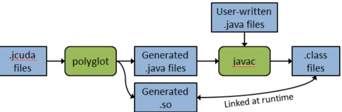
The JCUDA compiler performs source-to-source translation of JCUDA programs like the one shown in Figure 3.1 to Java programs. The implementation is built on Polyglot [20], a compiler front end for the Java programming language. The build process for a JCUDA program is shown in Figure 3.2. The initial inputs are JCUDA files like the example shown in Figure 3.1. Polyglot converts JCUDA files to auto-generated Java and C source code which include any JNI, CUDA, or JCUDA runtime API calls. The generated C files are then transparently compiled into a shared object library. At this point, the programmer builds the generated Java files with the option
∗Four angle brackets are used instead of three as in CUDA syntax because the “>>>” is already used as unsigned right shift operator in Java programming language.
1 double[ ][ ] l_a = new double[NUM1][NUM2];
2 double[ ][ ][ ] l_aout = new double[NUM1][NUM2][NUM3];
3 double[ ][ ] l_aex = new double[NUM1][NUM2];
4
5 initArray(l_a); initArray(l_aex); //initialize value in array
6
7 int [ ] ThreadsPerBlock = {16, 16, 1};
8 int [ ] BlocksPerGrid = new int[3];
9 BlocksPerGrid[0] = (NUM1 + ThreadsPerBlock[0] - 1) /
10 ThreadsPerBlock[0];
11 BlocksPerGrid[1] = (NUM2 + ThreadsPerBlock[1] - 1) /
12 ThreadsPerBlock[1];
13 BlocksPerGrid[2] = 1;
14
15 /* invoke device on this block/thread grid */
16 cudafoo.foo1<<<<BlocksPerGrid, ThreadsPerBlock>>>>(
17 l_a, l_aout, l_aex);
18 printArray(l_a); printArray(l_aout); printArray(l_aex);
... ... ...
90 static lib cudafoo ("cfoo", "/opt/cudafoo/lib") {
91 acc void foo1 (IN double[ ][ ]a, OUT int[ ][ ][ ] aout,
92 INOUT float[ ][ ] aex);
93 acc void foo2 (IN short[ ][ ]a, INOUT double[ ][ ][ ] aex,
94 IN int total);
95 }
Figure 3.2 : Build process for a JCUDA program
of including user-written Java files in the build process. User-written Java can call JCUDA methods. The final outputs of the JCUDA build process are a collection of Java CLASS files which are linked with the generated library at runtime.
Figures 3.3 and 3.4 show the Java static class declaration and the C glue code generated from the lib declaration in Figure 3.1. The Java static class introduces declarations with mangled names for native functions corresponding to JCUDA func-tions foo1 and foo2 respectively, as well as a static class initializer to load the stub library. In addition, three parameters are added to each call — dimGrid, dimBlock,
and sizeShared — corresponding to the CUDA grid geometry, block geometry, and
shared memory size. Figure 3.4 shows the generated C code with host-device trans-fers in accordance with the IN, OUT and INOUT modifiers in Figure 3.1. Note the
use of JCUDA library functions copyArrayJVMToDevice, copyArrayDeviceToJVM, allocArrayOnDevice, and freeDeviceMem. These functions wrap cudaMemcpy, cudaMalloc, and cudaFree. copyArrayJVMToDevice and copyArrayDeviceToJVM are useful because they take multi-dimensional Java arrays as input rather than C pointers, and can infer the dimensionality and size of the input or output array using JNI.
private static class cudafoo {
native static void HelloL_00024cudafoo_foo1(double[ ][ ] a, int[ ][ ][ ] aout, float[ ][ ] aex, int[ ] dimGrid, int[ ] dimBlock, int sizeShared);
static void foo1(double[ ][ ] a, int[ ][ ][ ] aout, float[ ][ ] aex, int[ ] dimGrid, int[ ] dimBlock, int sizeShared) {
HelloL_00024cudafoo_foo1(a, aout, aex, dimGrid, dimBlock, sizeShared);
}
native static void HelloL_00024cudafoo_foo2(short[ ][ ] a, double[ ][ ][ ] aex, int total, int[ ] dimGrid,
int[ ] dimBlock, int sizeShared);
static void foo2(short[ ][ ] a, double[ ][ ][ ] aex, int total, int[ ] dimGrid, int[ ] dimBlock, int sizeShared) {
HelloL_00024cudafoo_foo2(a, aex, total, dimGrid, dimBlock, sizeShared);
}
static{java.lang.System.loadLibrary("HelloL_00024cudafoo_stub");} }
extern __global__ void foo1(double * d_a, signed int * d_aout, float * d_aex);
JNIEXPORT void JNICALL
Java_HelloL_00024cudafoo_HelloL_100024cudafoo_1foo1(JNIEnv *env, jclass cls, jobjectArray a, jobjectArray aout, jobjectArray aex, jintArray dimGrid, jintArray dimBlock, int sizeShared) {
/* copy array a to the device */ int dim_a[3] = {2};
double * d_a = (double*) copyArrayJVMToDevice(env, a, dim_a, sizeof(double));
/* Allocate array aout on the device */ int dim_aout[4] = {3};
signed int * d_aout = (signed int*) allocArrayOnDevice(env, aout, dim_aout, sizeof(signed int));
/* copy array aex to the device */ int dim_aex[3] = {2};
float * d_aex = (float*) copyArrayJVMToDevice(env, aex, dim_aex, sizeof(float));
/* Initialize the dimension of grid and block in CUDA call */ dim3 d_dimGrid; getCUDADim3(env, dimGrid, &d_dimGrid);
dim3 d_dimBlock; getCUDADim3(env, dimBlock, &d_dimBlock); foo1<<<d_dimGrid, d_dimBlock, sizeShared>>> ((double *)d_a,
(signed int *)d_aout, (float *)d_aex); freeDeviceMem(d_a);
/* copy array d_aout-> aout from device to JVM */ copyArrayDeviceToJVM(env, d_aout, aout, dim_aout,
sizeof(signed int)); freeDeviceMem(d_aout);
/* copy array d_aex-> aex from device to JVM */
copyArrayDeviceToJVM(env, d_aex, aex, dim_aex, sizeof(float)); freeDeviceMem(d_aex);
}
sented as an array of arrays. For example, a two-dimensional float array is represented as a one-dimensional array of objects, each of which references a one-dimensional float array. This representation supports general nested and ragged arrays, as well as the ability to pass subarrays as parameters while still preserving pointer safety. However, it has been observed that this generality comes with a large overhead for the common case of multidimensional rectangular arrays [21].
This work focuses on the special case of dense rectangular two and three dimen-sional arrays of primitive types as in C and Fortran. These arrays are allocated as nested arrays in Java and as contiguous arrays in CUDA. The JCUDA runtime per-forms the necessary gather and scatter operations when copying array data between the JVM and the GPU device by iterating through the nested Java arrays using JNI and transferring them each to an offset in a pre-allocated device buffer. For example, to copy a Java array ofdouble[20][40][80] from the JVM to the GPU device, the JCUDA runtime makes 20×40 = 800 calls to the CUDAcudaMemcpy memory copy function with 80 double-words transferred in each call.
3.2
JCUDA Performance Evaluation
3.2.1 Experimental Setup
Three benchmarks from the Java Grande Forum (JGF) Benchmarks [22, 23] were used to evaluate the JCUDA programming interface and compiler — Fourier coeffi-cient analysis (Series), Sparse matrix multiplication (Sparse), and IDEA encryption (Crypt). Each of these benchmarks has three problem sizes for evaluation — A, B and C — with Size A being the smallest and Size C the largest. For each of these benchmarks, the compute-intensive portions were rewritten in CUDA while the rest of the code was retained in its original Java form, except for the JCUDA extensions
used for kernel invocation. The rewritten CUDA codes are parallelized in the same way as the original Java multi-threaded code.
The GPU used in these performance evaluations was a NVIDIA Tesla M2050, containing a GPU with 448 thread processors, a 1.15 GHz clock speed, and 2687MB of global memory. All benchmarks were evaluated with double-precision arithmetic, as in the original Java versions. The host of this GPU consists of a pair of 6-core Intel CPUs with a 2.80GHz clock speed and 48GB of RAM. The software used include a Sun Java HotSpot 64-bit virtual machine included in version 1.6.0 25 of the Java SE Development Kit (JDK), version 4.4.6 of the GNU Compiler Collection (gcc), version 304.54 of the NVIDIA CUDA driver, and version 5.0 of the NVIDIA CUDA Toolkit.
3.2.2 Evaluation and Analysis
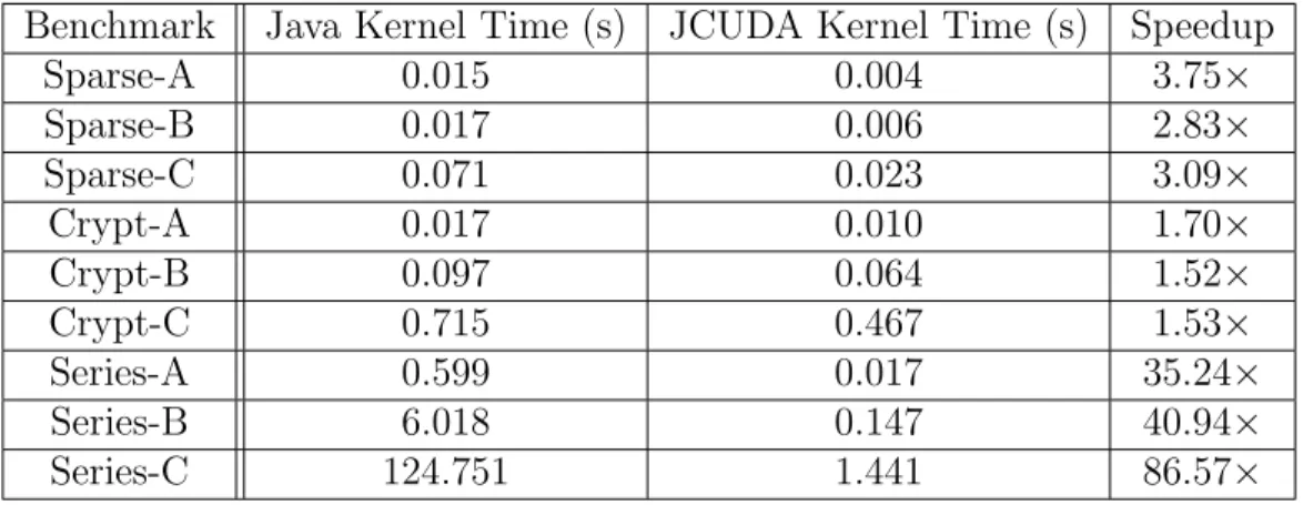
Table 3.1 shows the execution time of the multi-threaded Java and JCUDA versions for all three data sizes of each of the three benchmarks. The Java execution times were obtained using 12 threads on a 12 core CPU. The JCUDA execution times were obtained by using a single Java thread on the CPU combined with multiple threads on the GPU. The JCUDA and Java kernels were repeated 5 times, and the median time for each benchmark and test size is listed in the table.
The final column shows the speedup of the JCUDA version relative to the 12-threaded Java version. The results for Size C (the largest data size) show speedups ranging from 1.52×to 86.57×, whereas smaller speedups or slowdowns were obtained for smaller data sizes. The benchmark that showed the smallest speedup was Crypt. This is primarily due to poor memory access coherency in the device kernel and high CUDA initialization and cleanup overheads. In contrast, the Series examples show the largest speedup because it is an embarrassingly parallel application with a high ratio of computation to communication.
Sparse-B 0.017 0.006 2.83× Sparse-C 0.071 0.023 3.09× Crypt-A 0.017 0.010 1.70× Crypt-B 0.097 0.064 1.52× Crypt-C 0.715 0.467 1.53× Series-A 0.599 0.017 35.24× Series-B 6.018 0.147 40.94× Series-C 124.751 1.441 86.57×
Table 3.1 : Execution times in seconds, and Speedup of JCUDA relative to 12-thread Java executions
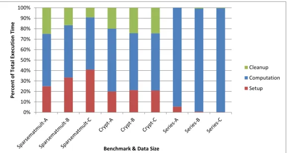
Figure 3.5 shows the percentage breakdown of JCUDA kernel execution times into computation, setup, and cleanup components. The computation component is the time spent in kernel execution on the GPU. The setup and cleanup components represent the time spent in data transfer before and after kernel execution. The figure shows that Series achieved the highest speedups due to large amounts of computation and little communications. Crypt and Sparse both demonstrated more moderate speedups from larger overheads due to data transfer.
3.3
Discussion
JCUDA can be used by Java programmers to invoke CUDA kernels by auto-generating JNI and CUDA bridge code at compile-time for programmer-written kernels operating on flat and multidimensional arrays. The JCUDA runtime handles data transfer to and from Java arrays. The performance results obtained on three Java Grande benchmarks show significant performance improvements of the JCUDA-accelerated versions over their original versions. In summary, JCUDA makes accelerating existing Java programs with many-core GPUs simple for programmers already familiar with writing CUDA kernels, while allowing many of the low-level optimizations required
0% 10% 20% 30% 40% 50% 60% 70% 80% 90% 100% P e rc e n t o f T o ta l E x e cu ti o n T im e
Benchmark & Data Size
Cleanup Computation Setup
Figure 3.5 : Percentage breakdown of JCUDA execution between CUDA setup, com-putation, and cleanup
Chapter 4
CnC-CUDA: Integrating CPU and GPU
Computation Into a Dataflow Language
While work on JCUDA made executing CUDA kernels on graphics hardware from Java applications a far simpler and natural process than was previously possible, it did little to add abstractions to the CUDA programming model for developers with little experience in CUDA.
CnC-CUDA extends Intel’s Concurrent Collections (CnC) programming model to address the challenge of efficiently executing workloads on a multi-architecture (hy-brid) platform by scheduling execution on CPUs and GPUs. CnC is a declarative and implicitly parallel coordination language that supports flexible combinations of task and data parallelism while retaining determinism. CnC computations are built using steps which are related by data and control dependence edges represented by a CnC graph. CnC-CUDA extends previous work on CnC-HJ, a multi-threaded CPU-only CnC implementation built on top of the parallel Habanero-Java (HJ) [24] runtime. The CnC-CUDA extensions to CnC-HJ include the definition of multi-threaded steps for execution on GPUs, as well as the automatic generation of data and control flow between CPU steps and GPU steps. By building support for heterogeneous processors into CnC-CUDA, higher-level abstractions can be provided to the user of heteroge-neous platforms than in JCUDA or other existing programming models. In addition, because of the dataflow nature of CnC and hints it is able to provide at runtime, CnC-CUDA can take advantage of a wider range of CnC-CUDA optimizations. Experimental results show that this approach can yield significant performance benefits with both
GPU execution and hybrid CPU/GPU execution.
4.1
Background on the CnC Model
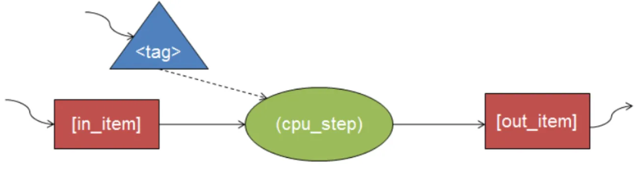
This section provides a brief summary of the CnC model, as described in [25]. A CnC program is a graph of sequential kernels, communicating with one another. The three main constructs in CnC are step collections, data item collections, and control tag collections. Statically, each of these constructs is acollection representing a set of dynamic instances. Step instances are the unit of distribution and scheduling. Item instances are the unit of synchronization and communication. Control tag instances are the unit of control. Figure 4.1 shows the relationships between these collections.
Figure 4.1 : Relationship between CnC tags, items, and computation steps
Control, data, and step instances are all identified by a unique tag within each collection. In CnC, tags are arbitrary values that support an equality test and hash function. Each type of collection uses tags as follows:
• Putting a tag into a control collection causes the corresponding steps (in the prescribed step collections) to eventually execute.
• Each step instance is a computation that takes a single tag (originating from the prescribing control collection) as an argument.
tag i, once written, cannot be overwritten (dynamic single assignment). The immutability of entries within a data collection is necessary for determinism. A CnC program is represented as a graph, stored in a textual graph file. Within the graph file, the CnC graph is represented using()to denote computation steps, [] to denote data items, and <> to denote control tags. The edges in the graph specify the partial ordering constraints required by the semantics. One type of ordering constraint arises from a data dependence. This relationship occurs when an instance of a step, produces an instance of an item which is later consumed by an instance of another step. Clearly the producing step instance must occur before the consuming step instance. Another type of ordering constraint arises from a control dependence, where one computation step instance determines if another computation step instance will execute. In that case, the controller step puts a control tag in a tag collection, which in turn prescribes the controllee step. The execution order of step instances is constrained only by their dynamic data and control dependences.
As an example, consider the CnC graph file in Figure 4.2. This graph file de-scribes a cryptographic benchmark (Crypt) from the JGF benchmark suite which first encrypts and then decrypts a string of characters. Included in the graph file are four item collections, two computation steps, and two tag collections. [plain]is the original, unencrypted input. [z]and [dk] are the keys used for encryption and decryption, respectively. crypt is the encrypted string. plain2 is the final decrypted output, which is identical to the original input in [plain]. The computation steps for encrypting and decrypting data are represented by (encrypt) and (decrypt). The creation of instances of these computation steps is controlled by puts into the <crypt tag> and <decrypt tag> tag collections. The control and data dependen-cies of Crypt are expressed on lines 14 and 15 in Figure 4.2. Also note the special
1 # Crypt CnC Graph File 2 3 env -> [plain]; 4 env -> [z]; 5 env -> [dk]; 6 7 [plain2] -> env; 8 9 env -> <crypt_tag>; 10 11 <crypt_tag>::(encrypt); 12 <decrypt_tag>::(decrypt); 13
14 [plain],[z] -> (encrypt) -> [crypt],<decrypt_tag>; 15 [crypt],[dk] -> (decrypt) -> [plain2];
Figure 4.2 : An example CnC graph file for the Crypt benchmark
env variable. env is used to indicate values that are either produced or consumed by the host application. Since all items and tags can be passed as generic Objects in CnC-HJ, the CnC graph file in Figure 4.2 contains no type information. Type information is necessary for CnC-CUDA extensions because of static, compile-time typing in CUDA.
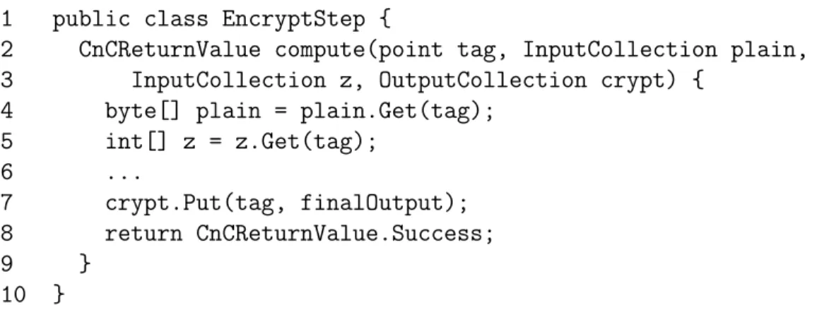
In addition to the CnC graph file, a CnC programmer must also define an entry point to the application and the implementation for each computational kernel. In CnC-HJ, the entry point is provided by a Java class that defines public static void main, within which the initial Puts and final Gets are done on item and tag collections (as described by the use of env in the graph file). The computation step implementations are also provided by Java classes. Each computation step definition must implement a compute function which defines the logic performed on a single CnC tag and its associated items. Abridged examples of a CnC entry point and computation step for Crypt are shown in Figures 4.3 and 4.4. Note the use of Put
item collection in line 26. In Figure 4.3, the notation [i] declares an HJ range. An HJ range can represent a scalar or multidimensional range of values. [i] represents a range including only one value, the value of i. [0:N-1] would represent a one-dimensional range of values including all integers from 0 to N-1, inclusive.
4.2
CnC-CUDA Design and Implementation
CnC-CUDA includes several extensions to the CnC programming model to support CUDA steps.
4.2.1 Graph File
Some of the features added require new syntax in the graph file. First, a new syntax is introduced for CUDA steps. CUDA steps are declared with braces, {}, instead of the parentheses, (), used for CPU steps.
Second, support for type specification in the CnC graph file is added for item and tag collections. This is necessary for auto-generation of CUDA and JNI API calls at compile-time.
Third, support was added for the definition of constants in the graph file using the following notation:
|const name const value|;
where const value is an integer. This definition generates constant values that can be referenced from both HJ and CUDA. These constants are used for specifying the exact size of item and tags that are passed to CUDA, ensuring the copying of the correct amount of data from Java arrays onto the CUDA device. For example, if each CUDA thread executing a CnC step takes 1000 integers, this item collection would be declared as:
1 public class CryptMain {
2 public static void main(String[] args) { 3 EncryptStep encrypt = new EncryptStep(); 4 DecryptStep decrypt = new DecryptStep();
5 cryptGraph graph = cryptGraph.Factory(encrypt,
6 decrypt);
7
8 byte[] plain = ...; 9 int[] z = ...; 10 int[] dk = ...;
11 byte[] plain2 = new byte[N]; 12 13 for(int i = 0; i < N; i++) { 14 graph.plain.Put([i], plain); 15 graph.z.Put([i], z); 16 graph.dk.Put([i], dk); 17 } 18 19 finish { 20 for(int i = 0; i < N; i++) { 21 graph.crypt_tag.Put([i]); 22 } 23 } 24 25 for(int i = 0; i < N; i++) { 26 plain2[i] = graph.plain2.get([i]); 27 } 28 validate(plain, plain2); 29 } 30 }
2 CnCReturnValue compute(point tag, InputCollection plain, 3 InputCollection z, OutputCollection crypt) {
4 byte[] plain = plain.Get(tag); 5 int[] z = z.Get(tag); 6 ... 7 crypt.Put(tag, finalOutput); 8 return CnCReturnValue.Success; 9 } 10 }
Figure 4.4 : Example of a computation step definition in the Crypt application
[int items[1000]];, or |size 1000|; [int items[size]];
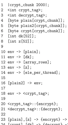
These extensions to the CnC graph file are illustrated in a modified and more verbose Crypt graph file in Figure 4.5. Note the declaration of type and size for the item and tag collections in lines 2–8, and the use of {}on lines 23 and 24 to indicate that encrypt and decrypt are now CUDA computation steps.
4.2.2 Item Collections
To enforce strict typing of items and tags, HJ definitions for all item collections are automatically generated by the CnC Parser at compile time. Item collections retain Put and Get methods for adding and retrieving individual items. In the CnC-CUDA implementation, each item is put into a ConcurrentHashMap. Once the number of buffered tags reaches a threshold, the items corresponding to those tags are collected from the ConcurrentHashMap, converted to a native format (i.e., java.lang.Integer→int) and passed to CUDA. While this approach is correct, the in-dividual accumulation and conversion of potentially large numbers of tags and items is inefficient.
1 |crypt_chunk 2000|; 2 <int crypt_tag>; 3 <int decrypt_tag>; 4 [byte plain[crypt_chunk]]; 5 [byte plain2[crypt_chunk]]; 6 [byte crypt[crypt_chunk]]; 7 [int dk[52]]; 8 [int z[52]]; 9 10 env -> [plain]; 11 env -> [dk]; 12 env -> [array_rows]; 13 env -> [z]; 14 env -> [ele_per_thread]; 15 16 [plain2] -> env; 17 18 env -> <crypt_tag>; 19 20 <crypt_tag>::{encrypt}; 21 <decrypt_tag>::{decrypt}; 22
23 [plain],[z] -> {encrypt} -> [crypt],<decrypt_tag>; 24 [crypt],[dk] -> {decrypt} -> [plain2];
eliminates putting and then extracting individual items, and the array can be directly passed to the kernel. Currently only arrays of primitive types are supported (int[], float[], etc.).
4.2.3 Tag Collections
Tag collections are automatically generated using type definitions in the graph file. The preliminary implementation only supports integer tags. This can be easily ex-tended to any hashable type, as in traditional CnC.
As described in Section 4.1, tag collections control the execution and synchroniza-tion of computasynchroniza-tion steps. New techniques must be used to support synchronizasynchroniza-tion between CUDA computation steps using tag collections. First, a pthread mutex is used to indicate that the device is currently in use by a computation step and inac-cessible by any new computation steps for GPU architectures which do not support concurrent kernel execution. Second, the number of CUDA computation steps that can be prescribed by another CUDA computation step is limited to 1, simplifying the complexity of synchronizing CUDA computation steps. If a CUDA step prescribes another CUDA step (as determined by analyzing the CnC graph file), the second step is invoked immediately following the first without returning to HJ. No limitation is placed on a CUDA step prescribing multiple HJ steps.
Like item collections, tag collections also implement the PutRegion operation. PutRegion immediately launches a CUDA kernel for all tags in the range once the required items are available. On individual tag Puts, the tag collection waits for a threshold number of tags to be put, and then launches a CUDA kernel with those tags and their associated items. This threshold has been empirically set to 8192 tags. Once all tags have been put into a GPU tag collection, the programmer has to issue
a call to that tag collection’s Wait() function to be certain that all CUDA threads have completed and their results have been returned to host memory.
The conceptual changes to the CnC graph dependencies caused by these changes to tag and item collections are illustrated in Figure 4.6. An example of the modifications required for the the CnC entry point from Figure 4.3 is shown in Figure 4.7.
Figure 4.6 : Relationship between CnC-CUDA tags, items, and computation steps with the added PutRegion/GetRegion primitives
For more advanced CUDA programmers the option of defining a two dimensional tag is provided:
<int tag:two region>
This offers the opportunity of placing a tag with 2 regions on the graph. Those two regions are interpreted as number of threads per thread group and number of groups per kernel invocation. In addition, the desired number of threads per thread group can be specified by compiling the graph file with the flag: -t <number of threads>.
1 public class CryptMain {
2 public static void main(String[] args) { 3 EncryptStep encrypt = new EncryptStep(); 4 DecryptStep decrypt = new DecryptStep(); 5 cryptGraph graph = cryptGraph.Factory(); 6 7 byte[] plain = ...; 8 int[] z = ...; 9 int[] dk = ...; 10 11 graph.plain.PutRegion([0:N-1], plain); 12 graph.z.PutRegion([0:N-1], z); 13 graph.dk.PutRegion([0:N-1, dk); 14 15 finish { 16 graph.crypt_tag.PutRegion([0:N-1]); 17 } 18
19 byte[] plain2 = graph.plain2.GetRegion([0:N-1]) 20 validate(plain, plain2);
28 }
29 }
A novel item collection property One-For-All (OFA) is also supported, which passes the same data to each thread on a device, where each thread is prescribed by a different tag. This property follows the format:
[type item:ofa]
where type can be any supported data type. This can result in both considerable saving in device and host memory as well as better performance from less data transfer overhead.
4.2.4 CUDA Kernel
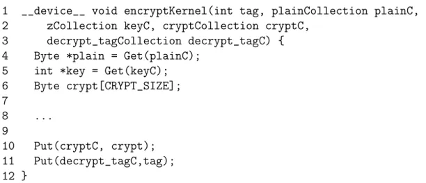
A CnC-CUDA programmer is responsible for providing CUDA kernels which imple-ment the functionality of CUDA computation steps. The CnC-CUDA compiler is responsible for generating stub codes that allocate memory and copy data to the de-vice before a step is executed. The auto-generated stub codes also free dede-vice memory after computation steps complete. The actual programmer-written step code is de-fined as a CUDA device function by the CnC programmer. The step function is called from an auto-generated CUDA kernel which serves as the CUDA entry point and protects against threads entering the programmer-defined kernel which do not have input. Threads which lack input are created when the number of CnC tags put is not evenly divisible by the selected thread group size. CUDA computation steps are limited to putting a single item on each output item collection. This limitation is a result of CUDA lacking dynamic memory allocation. An abridged example of a programmer-written CUDA computation step for the Crypt benchmark is shown in Figure 4.8.
2 zCollection keyC, cryptCollection cryptC, 3 decrypt_tagCollection decrypt_tagC) { 4 Byte *plain = Get(plainC);
5 int *key = Get(keyC); 6 Byte crypt[CRYPT_SIZE]; 7 8 ... 9 10 Put(cryptC, crypt); 11 Put(decrypt_tagC,tag); 12 }
Figure 4.8 : A code snippet from a CUDA computation step in the Crypt benchmark
4.2.5 Implementation Details
The CnC-CUDA Polyglot-based compiler builds a library of runtime and programmer-written CUDA and C procedures which communicate data and execute kernels. In CnC-CUDA, the complexity of inter-language function calls and device memory man-agement is hidden from the CnC programmer and auto-generated at compile time, allowing them to focus on developing and implementing the algorithms in their ap-plication.
There are two CUDA files generated from compile-time analysis of the CnC-CUDA graph file: cudaLaunchers.cuand kernelCallers.cu. cudaLaunchers.cuprovides the interface between CnC-HJ JVM execution and CUDA computation steps. Pseu-docode for the code auto-generated in cudaLaunchers.cu by the CnC-CUDA com-piler for an arbitrary computation step is shown in Algorithm 1. All of the in-formation needed to generate cudaLaunchers.cu is contained in the CnC-CUDA graph file. Page-locked CPU memory is used to permit asynchronous memory copies. Note that the functionality for transferring data between JVM¡-¿page-locked mem-ory and page-locked memmem-ory¡-¿CUDA is supported by runtime methods similar to the
1 __global__ void encryptKernelCaller(int *crypt_tag, 2 int num_crypt_tag, plainCollection *plain, 3 zCollection *z, cryptCollection *crypt, 4 decrypt_tagCollection *decrypt_tag) {
5 int tid = blockDim.x * blockIdx.x + threadIdx.x; 6
7 if(tid < num_crypt_tag) {
8 encryptKernel(crypt_tag[tid], *plain, *z, *crypt,
9 *decrypt_tag);
10 } 11 }
Figure 4.9 : An example computation step global function inkernelCallers.cu
copyArrayJVMToDeviceand copyArrayDeviceToJVMfunctions used in CnC-CUDA. kernelCallers.cu contains a CUDA global function for each computation step. These global functions pass control from the kernel launch in
cudaLaunchers.cu to the programmer-written CUDA kernels. The only purpose of kernelCallers.cuis to ensure CUDA threads with no input are blocked from enter-ing the computation step. An examplekernelCallers.cu is shown in Figure 4.9.
4.3
CnC-CUDA Performance Evaluation
To compare the performance of CnC-CUDA to CnC-HJ and other programming mod-els and languages three benchmarks were used: Fourier coefficient analysis (Series), IDEA encryption (Crypt), and Heart Wall Tracking. Series and Crypt come from the the Java Grande Forum (JGF) benchmark suite [26]. Heart Wall Tracking comes from the Rodinia benchmark suite [27]. Each benchmark was run on varying data sizes using some combination of CnC-CUDA, CnC-HJ, hand-coded CUDA, and ei-ther single-threaded Java (from JGF) or multi-threaded OpenMP (from Rodinia). Additionally, the Crypt benchmark was run in CnC-CUDA using CPU and GPU
totalMemReq = CalcM emoryF ootprintF orAllCollections() pageLockedHostBuffer = P ageLockedAlloc(totalM emReq) // Preparation
for collection in input items/tags do
Copy collection from JVM heap to offset in pageLockedHostBuffer deviceBufferi =DeviceAlloc(sizeof(collection))
end
for collection in output items/tags do
Preallocate device memory for outputs
end
// Host → Device
for collection in input items/tags do
Asynchronously copy from pageLockedHostBuffer → deviceBufferi
end
// Execute
Launch Asynchronous Kernel // Device → Host
for collection in output items/tags do
Asynchronously copy from deviceBufferi → pageLockedHostBuffer
end
Wait For Queued Work to Finish // Host → JVM
for collection in output items/tags do
Copy collection from pageLockedHostBuffer into JVM
end
// Cleanup
for collection in all items/tags do
if Not Used In Future Computation Steps then
F ree(collection)
end end
Algorithm 1: Pseudocode for the code generated for an arbitrary kernel in cudaLaunchers.cu
Crypt GPU Performance (s) CPU Performance (s)
Data Size (bytes) CnC-CUDA CUDA CnC-HJ Java Speedup (16 cores) 50,000,000 0.886 0.161 2.067 2.92 2.33 (JGF Size C) 75,000,000 1.208 0.253 3.239 4.387 2.68 100,000,000 1.488 0.341 4.460 5.818 3.00 150,000,000 2.311 0.550 6.903 8.716 2.99
Table 4.1 : Execution times in seconds of JGF Crypt benchmark implemented in several programming models, and Speedup of CnC-CUDA relative to CnC-HJ.
Series GPU Performance (s) CPU Performance (s)
Data Size CnC-CUDA CUDA CnC-HJ Java Speedup (16 cores)
10,000 0.332 0.0095 3.587 6.777 10.80
100,000 0.441 0.116 36.588 69.074 60.78
1,000,000 1.411 1.279 572.86 N/A 406.00
Table 4.2 : Execution times in seconds of JGF Series benchmark implemented in several programming models, and Speedup of CnC-CUDA relative to CnC-HJ.
computation steps in parallel. The timing of each benchmark was started just before the first set of tag puts were performed to launch the CnC graph or the function call to launch the actual computation for non-CnC benchmarks. Timing was stopped when all CnC steps completed or the core function completed. For GPU execution, these timings included the overhead of copying data to and from device memory.
For these evaluations, an NVIDIA GTX 480 GPU was used. The GTX 480 has 480 processing cores and 1.6 GB of memory. The CPU host of this GPU is 4 AMD Phenom 9850 Quad-Core Processors with a 1.25 GHz clock, 512 KB cache, and 8 GB of memory. The software used includes a Java HotSpot 64-bit virtual machine from version 1.6.0 20 of the Java Development Kit (JDK), a GNU C compiler v. 4.1.2, and version 3.1 of the NVIDIA CUDA Toolkit.
Heart Wall GPU Performance (s) CPU Performance (s)
Data Size CnC-CUDA CUDA CnC-HJ OpenMP Speedup
(# of frames) (16 cores) (16 cores)
1 0.427 0.985 0.246 0.005 0.57
104 4.4842 3.6133 11.058 13.863 2.47
Table 4.3 : Execution times in seconds on GPU - CnC-CUDA and hand-coded (Ro-dinia) CUDA versions - and CPU - Serial, OpenMP on 16 cores and CnC-HJ on 16 cores - of the Heart Wall Tracking benchmark.
Crypt Hybrid Performance (s)
Percent of Load Average Slowest Fastest Speedup
on GPU (Relative to CnC-CUDA)
10% 3.042 3.806 2.493 0.76 20% 3.066 3.765 2.727 0.75 30% 2.720 3.048 2.223 0.85 40% 2.289 2.750 1.878 1.01 50% 2.139 2.397 1.973 1.08 60% 2.035 2.242 1.538 1.14 70% 2.076 2.799 1.755 1.11 80% 2.189 2.511 1.883 1.06 90% 2.143 2.344 1.968 1.08
Table 4.4 : Execution times in seconds and Speedup of a hybrid CnC-CUDA/HJ version of Crypt against only CnC-CUDA.