Application of Machine Learning Algorithms to the Study of Noise Artifacts in Gravitational-Wave Data

(1)

Application of machine learning algorithms to the study of noise artifacts in gravitational-wave data

Rahul Biswas,1_{Lindy Blackburn,}2 _{Junwei Cao,}3 _{Reed Essick,}4 _{Kari Alison Hodge,}5_Erotokritos

Katsavounidis,4_{Kyungmin Kim,}6, 7_{Young-Min Kim,}8, 7_{Eric-Olivier Le Bigot,}3 _{Chang-Hwan Lee,}8 John J. Oh,7 Sang Hoon Oh,7 Edwin J. Son,7 Ruslan Vaulin,4 Xiaoge Wang,9and Tao Ye9

1_{University of Texas-Brownsville, Brownsville, Texas 78520, USA} 2_{NASA Goddard Space Flight Center, Greenbelt, MD 20771, USA} 3_{Research Institute of Information Technology, Tsinghua National Laboratory for}

Information Science and Technology, Tsinghua University, Beijing 100084, P. R. China

4_{LIGO - Massachusetts Institute of Technology, Cambridge, MA 02139, USA} 5_{LIGO - California Institute of Technology, Pasadena, CA 91125, USA}

6

Hanyang University, Seoul 133-791, Korea

7_{National Institute for Mathematical Sciences, Daejeon 305-811, Korea} 8_{Pusan National University, Busan 609-735, Korea}

9

Department of Computer Science and Technology, Tsinghua University, Beijing 100084, P. R. China The sensitivity of searches for astrophysical transients in data from the Laser Interferometer Gravitational-wave Observatory (LIGO) is generally limited by the presence of transient, non-Gaussian noise artifacts, which occur at a high-enough rate such that accidental coincidence across multiple detectors is non-negligible. Further-more, non-Gaussian noise artifacts typically dominate over the background contributed from stationary noise. These “glitches” can easily be confused for transient gravitational-wave signals, and their robust identification and removal will help any search for astrophysical gravitational-waves. We apply Machine Learning Algorithms (MLAs) to the problem, using data from auxiliary channels within the LIGO detectors that monitor degrees of freedom unaffected by astrophysical signals. Terrestrial noise sources may manifest characteristic disturbances in these auxiliary channels, inducing non-trivial correlations with glitches in the gravitational-wave data. The number of auxiliary-channel parameters describing these disturbances may also be extremely large; high dimen-sionality is an area where MLAs are particularly well-suited. We demonstrate the feasibility and applicability of three very different MLAs: Artificial Neural Networks, Support Vector Machines, and Random Forests. These classifiers identify and remove a substantial fraction of the glitches present in two very different data sets: four weeks of LIGO’s fourth science run and one week of LIGO’s sixth science run. We observe that all three al-gorithms agree on which events are glitches to within 10% for the sixth science run data, and support this by showing that the different optimization criteria used by each classifier generate the same decision surface, based on a likelihood-ratio statistic. Furthermore, we find that all classifiers obtain similar limiting performance, sug-gesting that most of the useful information currently contained in the auxiliary channel parameters we extract is already being used. Future performance gains are thus likely to involve additional sources of information, rather than improvements in the MLAs themselves.

I. INTRODUCTION

The Laser Interferometer Gravitational-wave Observa-tory (LIGO) is a two-site network of ground-based detec-tors designed for the direct detection and measurement of gravitational-wave signals from astrophysical sources [1, 2]. The LIGO detectors, in their initial configuration [1], have op-erated since 2001 and conducted several scientific runs, col-lecting data with incrementally increased sensitivity in each run [1, 3, 4]. Although no gravitational waves were detected, these runs tested and refined key technologies, as well as pro-vided a large amount of data characterizing the detectors. The next generation of detectors, referred to as the advanced LIGO detectors, are currently under construction and are expected to be operational by 2015 [1, 2]. Major upgrades to lasers, op-tics, and seismic isolation/sensing will provide roughly a fac-tor of ten improvement to sensitivity, which corresponds to a factor of 1000 in the observable volume of space and the num-ber of detectable sources. Based on our current knowledge of potential astrophysical sources, the advanced LIGO detectors are expected to make routine gravitational-wave detections (see, for example, [5]) and will open the era of gravitational-wave astronomy.

The LIGO detector noise may be characterized by an ap-proximately stationary component of colored Gaussian noise, with the addition of short duration non-Gaussian noise ar-tifacts called “glitches” (other noise sources such as non-stationary lines and broadband non-stationarity do not always ﬁt neatly into this framework). The stationary noise in the instrument is dominated by low-frequency seismic noise cou-pling to mirror motion, thermal noise in the mirrors and sus-pensions, 60 Hz power lines and harmonics, and shot noise. Sources of transient noise can include temporary seismic, acoustic, or magnetic disturbances, power transients, scattered light, dust crossing the beam, instabilities in the interferome-ter, channel saturations, and other complicated and often non-linear effects. To monitor these disturbances and keep the in-strument in a stable operating condition through active feed-back, each detector records hundreds of auxiliary channels along with the gravitational-wave channel. These auxiliary channels keep track of important non-gravitational-wave de-grees of freedom in the interferometer, as well as information about the local environment. They are critical to understand-ing the state of the instrument at any particular time.

One of LIGO’s main scientiﬁc goals is the detection of transient gravitational-wave signals, which can come from

(2)

the coalescence of a compact binary or core-collapse super-nova, among other astrophysical sources [6]. The presence of glitches is problematic for searches targeting these sig-nals because glitches can be easily confused with transient gravitational-wave signals. The primary method to distin-guish a real gravitational-wave transient from instrumental ar-tifact is to check that a signal appears in two or more geo-graphically distant detectors. While this coincidence require-ment is extremely effective, a high rate of glitches means that accidental coincidence of noise transients across multi-ple detectors still dominates the search background, result-ing in weaker upper limits and makresult-ing the conﬁdent detec-tion of real signals challenging. The problem is most se-vere in searches for transients with poorly-modeled or little identifying waveform structure, such as generic gravitational-wave bursts or intermediate-mass binary black-hole coales-cence which spend only a short amount of time (few cycles) in the LIGO sensitive band.

While the precise noise characteristics in the advanced de-tectors will be different from those of initial LIGO, glitch sources for future data will exist and the detection problem for short duration signals will persist. Thus, it is critical to develop data analysis methods for the robust identification of glitches in LIGO data. For previous investigations of instru-mental artifacts, their impact on gravitational-wave searches and the methods for their identification, see [7–14]. We use the Ordered Veto List (OVL) algorithm as a benchmark for our investigations. OVL has been used in recent LIGO sci-ence runs as one of the primary glitch detection algorithms. In particular, an earlier version of OVL described in [15] was used during LIGO’s fifth science run [16]. OVL attempts to measure the degree of likelihood that a gravitational wave can-didate can be associated with a transient instrumental distur-bance found in one of the many auxiliary channels.

Glitches are induced by the detector’s environment, noise in the detector subsystems, or a combination of thereof. These sources should appear in the auxiliary channels as well. Be-cause legitimate gravitational waves may couple to channels besides the nominal gravitational wave channel, we use a sub-set of auxiliary channels shown to be insensitive to gravita-tional waves. This subset is generated through hardware in-jections at the detectors [13]. The hardware inin-jections involve driving the test masses through magnetic coupling with an ex-pected gravitational wave signal and searching for evidence of that signal in auxiliary channels. If the signal does not systematically appear in an auxiliary channel, that channel is deemed “safe” and we include it in our analysis. By analyz-ing information from these auxiliary channels, one may be able to distinguish glitches from genuine gravitational-wave signals and ideally establish their cause. The main difﬁculty in such an analysis is processing the information from hun-dreds of channels which may manifest non-trivial correlations between themselves when they respond to an instrumental disturbance. Given the high dimensionality and the absence of reliable statistical models for noise and coupling between auxiliary channels, traditional computational methods are not well-suited to this problem. On the other hand, Machine learn-ing algorithms (MLA)s have been used to solve problems like

this since the 1970’s in other ﬁelds such as computer science, biology, and ﬁnance.

This paper presents the use of MLAs for the purpose of glitch identification in gravitational-wave detectors. The main goal of the paper is to establish the feasibility of apply-ing MLAs in the context of the LIGO detectors. We con-sider three well-known algorithms: the Artificial Neural Net-work (ANN), the Support Vector Machines (SVM), and the Random Forest (RF). We explore their properties and test their performance by analyzing data from past scientific runs. Based on these tests, we discuss the prospects for using MLAs for glitch identification in the advanced LIGO detectors.

This paper is organized as follows. In Section II, we describe the process for reducing raw time-series data and preparing feature vectors for the MLA classifiers. This is fol-lowed by a general formulation of the glitch detection prob-lem in Section III. Then, in Section IV, we briefly describe the classifiers’ algorithms. Training and testing of the classifiers is discussed in Section V. Finally, we evaluate and compare the classifiers’ performances using the standard Receiver Op-erating Characteristic (ROC) curves in Section VI and inves-tigate various ways of combining classifiers in Section VII. In Appendix A, we explore several optimization criteria used by the classifiers and verify their theoretical consistency.

II. DATA PREPARATION

We use data taken by the 4km-arm detector at Hanford, WA (H1) during LIGO’s fourth science run (S4: 24 February – 24 March 2005), and data taken by the 4km-arm detector at Livingston, LA (L1) during one week (28 May – 4 June 2010) of LIGO’s sixth science run (S6: 7 July 2009 – 20 October 2010). Hereafter we refer to these data sets as the S4 and the S6 data.

In the time between the fourth and the sixth science runs, the detectors underwent major commissioning and improve-ments to their sensitivity. Thus, while the H1 and L1 detec-tors are identical by design, the data taken by H1 during S4 and the data taken by L1 during S6 are quite different. These data sets represent evolutionary changes in both the detec-tor noise power-spectral-density and the non-Gaussian tran-sient artifacts. Differences in the detectors’ environments due to their distant geographical locations add another degree of freedom. Processing data from detectors separated in time and location allows us to determine how adaptable and robust these analysis algorithms are. This is important when extrap-olating their performance to advanced detectors.

Classification, or the separation of input data into various categories, is one of MLAs main uses; thus, they are often referred to as classifiers. We have two categories of data: glitches (Class 1) and “clean” data (Class 0). If one was to perform a search for gravitational-wave transient signals, the first category, glitches, would generally be identified as candi-date transient events and considered false alarms. The second category, “clean” data, contain only Gaussian detector noise. A true gravitational-wave signal, when it arrives at the detec-tor, is superposed on the Gaussian detector noise. If the

(3)

sig-nal’s amplitude is high enough, it also would be identiﬁed by the search algorithm as a candidate transient event. Since it is a genuine gravitational-wave transient, it would constitute an actual detection, as opposed to glitches which act as noise. Hereafter we refer to such candidate gravitational-wave tran-sient events, either genuine gravitational-wave trantran-sients or glitches, as transient events or simply as events.

We characterize a transient event in either class by infor-mation from the detector’s auxiliary channels. Importantly, we record the same information for both classes of events. Each channel records a time-series measuring some non-gravitational-wave degree of freedom, either in the detector or its environment. We first reduce the time-series to a set of non-Gaussian transients using the Kleine Welle analysis algo-rithm [17], which finds clusters of excess signal power in the dyadic wavelet domain. The detected transients are ranked by their statistical significance, defined as the negative loga-rithm of the probability that a random cluster of wavelet co-efficients subject to Gaussian noise would contain the same or greater signal power. The MLA classifiers use the proper-ties of auxiliary channel transients coincident in time with the wave channel event to classify the gravitational-wave event.

Given an event in the gravitational-wave channel at timet, we build a feature vectorxout of the nearby auxiliary channel transients. Each channel contributes ﬁve features:

• ρ: The signiﬁcance of the single loudest transient in that auxiliary channel within±100 ms oft.

• Δt: The difference betweentand the central time cor-responding to the auxiliary channel transient.

• d: The duration of the auxiliary channel transient.

• f: The central frequency of the auxiliary channel tran-sient.

• n: The number of wavelet coefﬁcients clustered to form the auxiliary channel transient (a measure of time-frequency volume).

We require all auxiliary transients to have a significance of at least 15, and if no such auxiliary transient is found within 100 ms oft, the five fields for that channel are set to zero. The significance threshold of 15 and 100 ms window are tunable parameters. The 100 ms window covers most transient cou-pling timescales identified by previous studies [13]. However, there is no guarantee that this window is an optimal choice, or that it should be the same for all auxiliary channels. In total, we analyze 250 (162) auxiliary channels from S6 (S4) data, re-sulting in 1250 (810) dimensions for the auxiliary feature vec-tor,x. In addition, we record certain bookkeeping information about the original gravitational-wave channel event, the state of nearby non-Gaussian transients in the gravitational-wave channel, and other information about data quality. These val-ues are stripped before classifier training and evaluation so that we train the classifiers on only information contained in the auxiliary features.

The set of “glitch” (Class 1) samples,{x}1, is generated

by running Kleine Welle over the gravitational-wave channel

from one of the LIGO detectors. This set of non-Gaussian transients from the gravitational-wave channel can, in prin-ciple, contain true gravitational-waves. However, prior to the coincidence requirement, they are overwhelmingly dominated by noise artifacts. Even for the most sensitive data set (S6), the expected rate of detectable gravitational-wave transients from known astrophysical sources is extremely low (∼10−9

Hz [5]) with respect to the rate of single-detector noise tran-sients (∼0.1Hz). For the advanced LIGO detectors, it may be appropriate to remove coincident gravitational-wave can-didates from the glitch training samples to avoid contamina-tion from detectable gravitacontamina-tional-wave events. In both classi-ﬁers’ training and performance evaluation, we treat all Kleine Welle transients from the gravitational-wave channel as ar-tifacts. In total, we identify 2832 (16,204) noise transients above a nominal signiﬁcance threshold of 35 from the Liv-ingston L1 (Hanford H1) detector during one week of the S6 (four weeks of the S4) science run. The central time from each event is used to trigger feature vector generation, so that{x}1

is a set of 2832 (16,204) sample vectors, each described by 1250 (810) features derived from coincident auxiliary chan-nel information. The samples are most representative of the background in gravitational-wave burst searches which gener-ally target short, unmodeled signals.

“Clean” (Class 0) samples,{x}0, are formed by ﬁrst

gen-erating 105 _{randomly distributed times within the data from}

each detector, producing a Poisson distribution mimicking (at a greatly exaggerated rate) that which would come from a set of true gravitational-wave signals (ignoring effects like detec-tor sensitivity). It can also be seen as a sampling of times when there was no glitch in the gravitational-wave channel, and will sample the typical auxiliary transients that do not produce a gravitational-wave glitch. To further aid in distin-guishing times when there is no disturbance, we exclude Class 0 samples which fall within±100 ms of a Class 1 sample. As with Class 1, the full set of Class 0 samples{x}0is built from

auxiliary channel information nearby each randomly selected time.

III. GENERAL FORMULATION OF THE DETECTION PROBLEM

The data analysis problem which we address here can be formulated as the robust identification of transient artifacts (glitches) in the gravitational-wave channel based on the in-formation contained solely in the safe auxiliary detector chan-nels. Clearly, the solution to this problem is directly related to the solution to the ultimate problem of robust detection and classification of gravitational-wave transients in LIGO data. The identification of glitches will reduce the non-Gaussian background and improve the sensitivity of gravitational-wave searches.We leave the question of how the results of our cur-rent analysis of the auxiliary channels can be incorporated into the search for transient gravitational waves to future work.

For a given transient event in the gravitational-wave chan-nel, we construct a feature vector of auxiliary information,x, following the procedure outlined in Section II. Our detection

(4)

problem reduces to binary prediction on whether this transient is a glitch (Class 1) or a clean sample (Class 0) based onxand onlyx. In feature-space,x∈Vd, this binary decision can be

mapped into identifying domains for Class 1 events,V1, and

Class 0 events, V0. We call the surface separating the two

regions the decision surface. Unless the two classes are per-fectly separable, which is typically not the case, there is a non-zero probability for an event of one class to occur in a domain identified with a different class. In this case, one would like to find an optimal decision surface separating two classes in such a way that we maximize the probability of finding events of Class 1 inV1at fixed probability of miscatagorizing events

from Class 0 inV1. This essentially minimizes the probability

of incorrectly classifying events. P1represents the

probabil-ity of glitch detection, which we also calldetection efﬁciency, andP0 is called thefalse alarm probability. This

optimiza-tion principle is often referred to as the Neyman-Pearson cri-teria [18].

The probability of detection and the probability of false alarm can be expressed in terms of conditional probability density functions for the feature vector,x:

P1= Vd Θ (f(x)−F∗)p(x|1)p(1) dx , (1a) P0= Vd Θ (f(x)−F∗)p(x|0)p(0) dx . (1b) Herep(x|1)andp(x|0)define probability density functions for the feature vector in the presence and absence of a glitch in the gravitational-wave data, respectively.p(1)and p(0)are prior probabilities for having a glitch or clean data, related to one another viap(1) +p(0) = 1.Θ (f(x)−F∗)defines the region V1 which signifies a glitch in the gravitational-wave

data, andf(x) = F∗ deﬁnes the decision surface. F∗ is a threshold parameter, which corresponds to a speciﬁc value of the probability of false alarm through (1b).

The optimal decision surface is found by maximizing the functional

S[f(x)] =P1[f(x)]−l0(P0[f(x)]−P0∗), (2)

whereP0∗is a tolerable value for the probability of false alarm

andl0 is a Lagrange multiplier. Setting the variation of this

functional with respect tof(x)to zero leads to the condition for the points on the decision surface that

p(x|1)p(1)

p(x|0)p(0) =CONSTANT. (3)

The ratio of conditional probability density functions, Λ(x)≡p(x|1)

p(x|0), (4)

is called the likelihood ratio (sometimes also referred to as the Bayes factor). TheCONSTANTin the optimality condition (3) does not carry any special meaning, and the condition can be satisﬁed if the decision surface is deﬁned as the surface of constant likelihood ratio [19],

f(x) = Λ(x) =F∗, (5)

withF∗ set by the probability of false alarm, P0∗, through

(1b). Actually, the decision surface can be deﬁned by any monotonic function of the likelihood ratio with trivial redeﬁ-nition ofF∗. There is a unique decision surface for each value ofP0∗∈[0,1], and we can label decision surfaces by their

cor-responding values ofP0∗.

The optimization of (2) maximizes the detection probabil-ity,P1 → P1OPT, for every value of the probability of false

alarm, P0 = P0∗. The curve P1OPT(P0) is called the

Re-ceiver Operating Characteristic (ROC) curve. It is a standard measure of any detection algorithm’s performance. We can think of optimizing (2) as maximizing the area under the ROC curve. For further details on use of the likelihood ratio in the gravitational-wave searches, see [19, 20].

Finding the optimal decision surfaces by direct estimation of the conditional probability density functions,p(x|1)and p(x|0), is an extremely difﬁcult task if the feature vector con-tains more than a few dimensions. For high-dimensional prob-lems, when no parametric model for these probability distri-butions is known and with a limited number of experimental samples that can be used to estimate these probability density functions, one has to resort to some other method. MLAs are well-suited for these detection problems.

In this paper, we consider three popular MLAs: ANN, SVM and RF. They differ significantly in their underlying algorithms and their approaches to classification. This allows us to investigate the applicability of different types of MLAs to glitch identification in the gravitational-wave data. How-ever, all MLAs require training samples of events from both Class 1 and Class 0. The MLA classifiers use the training sets to find an optimal classification scheme or decision surface. In the limit of infinitely many samples and unlimited computa-tional resources, different classifiers should recover the same theoretical result, the decision surface defined by the constant likelihood ratio (5). To this end, it is critical that classifiers are trained and optimized using criteria consistent with this result. In Appendix A, we explore several standard optimiza-tion criteria and derive the decision surfaces they generate in this theoretical limit. We find that all of these criteria lead to a decision surface with constant likelihood ratio. In particular, this is true for the fraction of correctly classified events and the Gini index criteria that are used by ANN / SVM and RF, respectively.

While all classifiers we investigate here should find the same optimal solution with sufficient data, in practice, the al-gorithms are limited by the finite number of samples in the training sets and by computational cost. The classifiers have to handle a large number of dimensions efficiently, many of which might be redundant or irrelevant. By no means is it clear that the MLA classifiers will perform well under such conditions. It is our goal to demonstrate that they do.

We evaluate their performance by computing ROC curves. 1_{These curves, which map the classiﬁers’ overall efﬁciencies,} are objective and can be directly compared. In addition to

1_{More traditional veto approaches to data quality in gravitational-wave}

(5)

configu-comparing the MLA classifiers to each other, we benchmark them using ROC curves from the OVL algorithm [21]. This method constructs segments of data to be vetoed using a hard time window and a threshold on the significance of transients in the auxiliary channels. The veto segments are constructed separately for different auxiliary channels and are applied in the order of decreasing correlation with the gravitational-wave events. By construction, only pairwise correlations be-tween a single auxiliary channel and the gravitational-wave channel are considered by the OVL algorithm. These results have a straightforward interpretation and provide a good san-ity check.

In order to make the classiﬁer comparison as fair as possi-ble, we train and evaluate their performances using exactly the same data. Furthermore, we use a round-robin procedure for the training-evaluation cycle, which allows us to use all avail-able glitch and clean samples. Samples are randomized and separated into ten equal subsets. To classify events in thekth subset, we use classiﬁers trained on all but thekthsubset. In this way, we ensure that training and evaluation are done with disjoint sets so that any over-training that might occur does not bias our results.

An MLA classiﬁer’s output is called a rank,rMLA ∈[0,1], and a separate rank is assigned to each glitch and clean sam-ple. Higher ranks generally denote a higher conﬁdence that the event is a glitch. A threshold on this rank maps to the probability of false alarm,P0, by computing the fraction of

clean samples with greater or equal rank. Similarly, the prob-ability of detection or efﬁciency,P1, is estimated by

comput-ing fraction of glitches with greater or equal rank. Essentially, we parametrically deﬁne the ROC curve, POPT

1 (P0), with a

threshold on the classifier’s rank. Synchronous training and evaluation of the classifiers allow us to perform a fair compar-ison and to investigate various ways of combining the outputs of different classifiers. We discuss our findings in detail in Sections VI and VII.

IV. OVERVIEW OF THE MACHINE LEARNING ALGORITHMS

In this section, we give a short overview of the basic prop-erties of the classifiers and the tuning procedures used to de-termine the best performing configurations for each classifier. Throughout this section, we will use the notation xi where i = 1,2, ...N to denote the set of N sample feature vectors. Similarly, yi will denote the actual class associated with the

ration consisting of a list of disjoint segments of data, the fractional “dead-time” is computed from the sum of the durations of all data segments to be vetoed. While not precisely the same, this quantity is related to the proba-bility of false alarm,P0, which accounts only for the fraction of clean data removed from the search. For a typical rate of glitches of∼0.1Hz, the two

measures are almost identical in the most relevant region ofP₀ ≤0.01.

Thus, in that interval the ROC curves of this paper can be directly com-pared to the often used ﬁgure of merit, efﬁciency vs. fractional dead-time. See for example [13].

theith_{sample feature vector, either Class 0 or Class 1.}

Predic-tions about a feature vector’s class will be denoted byy(xi).

A. Artiﬁcial Neural Network

ANNs employ a machine learning technique based on sim-ulating the data processing in human brains and mimicking biological neural networks [22, 23]. As is well-known, the human brain is composed of a tremendous number of inter-connected neurons, with each cell performing a simple task (responding to an input stimulus). However, when a large number of neurons form a complicated network structure, they can perform complex tasks such as speech recognition and decision-making.

A single neuron is composed of dendrites, a cell body, and an axon. When dendrites receive an external stimulus from other neurons, the cell body computes the signal. When the to-tal strength of the stimulus is greater than the synapse thresh-old, the neuron is fired and sends an electrochemical signal to other neurons through the axon. This process can be imple-mented with a simple mathematical model including nodes, a network topology and learning rules adopted to a specific data processing task. Nodes are characterized by their num-ber of inputs and outputs (essentially how many other nodes they talk to), and by the connecting weights associated with each input and output. The network topology is defined by the connections between the neurons (nodes). The learning rules prescribe how the connecting weights are initialized and evolve.

There are a large number of ANN models with different topologies. For our purpose, we choose to implement the multi-layered perceptron (MLP) model, which is one of the most widely used models. The MLP model has input and out-put layers as well as a few hidden layers in between. The in-put vector for the inin-put layer is the auxiliary feature vector,x, while the input for hidden layers and the output layer is a com-bination of the output from nodes in the previous layer. We will call these intermediate vectorszto distinguish them from the full feature vector. Each layer has several neurons which are connected to the neurons in the adjacent layers with indi-vidual connecting weights. The initial structure - the number of layers, neurons, and the initial value of connecting weights - is chosen by hand and / or through an optimization scheme such as a genetic algorithm (GA).

When a neuron’s input channels receive an external signal exceeding the threshold value set by an activation function, the neuron is ﬁred. This process can be expressed mathematically as:

y(z) =f(w·z+b), (6) wherey(z)is the output,zis an input vector,ware connect-ing weights,f is an activation function, andbis a bias. One may choose the activation function to be either the identity function, the ramp function, the step function, or a sigmoid

(6)

function. We use the sigmoid function deﬁned by f(w·z+b) = 1 + e−2s(w·z+b) −1 . (7)

We set the activation steepnesss = 0.5 in hidden layers ands= 0.9at the output layer. There is a single neuron at the output layer, and the value of that neuron’s activation function is used as ANN’s rank,rANN.

The topological parameters determine the number of con-nection weights, which must be sufﬁciently large that ANN has enough degrees of freedom to classify a given datum. The network’s ﬂexibility depends on the number of connection weights and should be matched with the size of the training sets and the input data’s dimensionality. In our work, the num-bers of layers and neurons are chosen so that the total number of connection weights is on the order of104_{when using the}

entire data set. In order to avoid overtraining, we decrease the number of layers and neurons in the runs in which either the dimensionality or the number of training samples are reduced. The learning scheme ﬁnds the optimal connection weights, w, in each layer. In this paper we use the improved version of the Resilient back PROPagation (iRPROP) algorithm [24], which minimizes the error between the output value, y(xi), and the known value,yi. In this algorithm, the increase (de-crease) factor and the minimum (maximum) step-size deter-mine the change in the connection weights,Δw, at each iter-ation during the training. In our work, the default values in theFANN!(FANN!) library [25] are used for all parameters except the increase factor, which is set toη+ _{= 1}_.₀₀₁_{. The}

same learning rules were used in all runs. We should note that ANNs can be optimized in an alternative way, via a GA or other similar methods. When using a GA, a combined opti-mization algorithm for topology, feature and weight selection can be applied to improve the performance of ANN [26–30]. We explore these options in a separate publication [31].

In addition to the choosing the ANN conﬁguration param-eters, we found that ANN requires data pre-processing. The input variables with high absolute values have a greater ef-fect on the output values, thus we normalize all components of the feature vector,x, to the range[0,1]. To better resolve smallΔtvalues,Δtis transformed via a logarithmic function before normalization.

Δt=−sign(Δt) log|Δt|. (8) This transformation improves ANN’s ability to identify glitches, which tend to have smaller values ofΔt. You can ﬁnd a more detailed description of the procedure for tuning the ANN conﬁguration parameters in [31].

B. Support Vector Machines

The SVM is an MLA for binary classiﬁcation on a vector space [32, 33]. It ﬁnds the optimal hyperplane that separates the two classes of training samples. This hyperplane is then

used as the decision surface in feature space, and classiﬁes events depending on which side of the hyperplane they fall.

As before, let{(xi, yi)|i= 1,2, ...N}be the training data set, wherexiis the feature vector of auxiliary transient infor-mation near timeti, andyi∈ {1,−1}is a label that marks the sample as either Class 1 or Class 0, respectively. Then assume that the training set is separable by a hyperplanew·x−b= 0, wherewis the normal vector to the hyperplane and bis the bias. Then the training samples withyi= 1satisfy the condi-tionw·xi−b≥1, and the training samples withyi=−1 sat-isfy the conditionw·xi−b≤ −1. SVM uses a quadratic pro-gramming method to ﬁnd thewandbthat maximize the mar-gin between the hyperplanesw·x−b= 1andw·x−b=−1. If the training samples are not separable in the original fea-ture space,Vd, SVM uses a mapping,φ(x), into a higher

di-mensional vector space, Vφ, in which two classes of events can be separated. The decision hyperplane inVφcorresponds to a non-linear surface in the original space,Vd. Thus,

map-ping the problem into a higher dimensional space allows SVM to consider non-linear decision surfaces. The dimensionality ofVφgrows exponentially with degree of the non-linearity of the decision surfaces inVd. As a result, SVM can not

con-sider arbitrary decision surfaces and usually has to deal with non-separable populations. If the training samples are not sep-arable after mapping, a penalty parameter,C, is introduced to weight the training error. Finding the optimal hyperplane is reduced to the following quadratic programming problem:

min w,b,ξ 1 2w·w+C N i=1 ξi , (9a) subject toyi·(w·φ(xi) +b)≥1−ξi, (9b) ξi≥0, i= 1,2, ..., N . (9c)

When the solution is found, SVM classiﬁes a samplexby the decision function:

y(xi) = sign (w·φ(xi) +b). (10) In solving the quadratic programming problem, the func-tion φ is not explicitly needed. It is sufﬁcient to specify φ(xi)·φ(xj). The functionK(xi, xj) =φ(xi)·φ(xj)is called the kernel function. The form of the kernel function implicitly deﬁnes the family of surfaces inVdover which SVM is

opti-mizing. In this study we use the Radial Basis function (RBF) as the kernel function. It is deﬁned as

K(xi, xj) = exp−γ||xi−xj||2 , (11) whereγis a tunable parameter.

The SVM algorithm was implemented by using the open-source package libsvm [34]. As part of this package, the kernel function parameter, γ, and the penalty parameter, C, are tuned in order to achieve the best performance for a spe-ciﬁc application. The best parameters (Candγ) are selected through an exhaustive search. For each pair of parameters (logC,logγ) on a grid, we calculate a ﬁgure of merit. The

(7)

parameters with the best figure of merit are then used for clas-sifying events. The default figure of merit in libsvm is the accuracy (fraction of correctly classified events). However, we replace it with a figure of merit better adapted to glitch de-tection. Instead of using the accuracy, our code calculates the area under the estimated ROC curve (PEST

1 (P0)) in the interval

of the probability of false alarmP0 ∈[0.001,0.05]on a

log-linear scale ([0.001,0.05]is a range of acceptable probability of false alarm for practical glitch detection).

ﬁgure of merit =

P0=0.05

P0=0.001

d (lnP0)P1EST(P0) (12)

Performing an exhaustive search for the best SVM parame-ters is computationally expensive. We can speed up this tuning process by exploiting the fact that the tuning time grows non-linearly with the training sample size. By using smaller train-ing sets, we can reduce the total time spent determintrain-ing the optimal parameters. We randomly selectedpsubsets of vec-tors from the training set, with each subset 10 times smaller than the full training set. The best pair of the SVM parame-ters for each of thepsubsets was then calculated, with each subset optimization running on a single CPU core. This gives psets of best parameters, calculated in parallel. The parame-tersC andγthat are selected the most often were then cho-sen as the ﬁnal best SVM parameters. This modiﬁed parame-ter optimization algorithm was applied to various training sets (described in Section V). We found that the optimal SVM pa-rameters do not depend on the training set. We, therefore, use the same parameters for all calculations reported in this paper (C= 8andγ= 0.0078125).

In its standard configuration, SVM classifies samples by a discrete label,y∈ {1,−1}. However, the libsvm package can provide a probability based version of (10) that yields con-tinuous values,rSVM ∈ [0,1][35]. We use these continuous values as the output of the SVM classifier.

C. Random Forest Technology

RF technology [36, 37] improves upon the classical deci-sion tree [38, 39] approach to classiﬁcation. The classifying decision tree performs a series of binary splits on any / all of the dimensions of the feature vector,x, that describes an event. The goal is to distribute events into groups consisting of only a single class. In a machine-learning context, the decision tree is formed by training it on a set of events of known class. Dur-ing the trainDur-ing, a series of splits are made, where each split chooses the dimension and its threshold that optimizes a cer-tain criterion, such as the fraction of correctly classiﬁed train-ing events or the Gini index. Splitttrain-ing stops once no split can further improve the optimization criterion or once the limit on the minimum number of events allowed on a branch (the fur-thest reaches of a decision tree) is reached; at this point the branch becomes a leaf. Once a tree is formed, an event of unknown class is fed into the tree, and depending on its fea-ture vector,x, it will be labeled as either Class 0 or Class 1.

However, a single decision tree can be a victim to both false minima and over-training. To guard against this, we create a forest of decision trees and average over their answers; this results in a continuous ranking,rRF ∈[0,1], rather than a bi-nary classiﬁcation, as events can be placed on a continuum between Class 0 and Class 1.

Each decision tree in the forest is trained on a bootstrap replica of the original training set. If the original training set has N events, each bootstrap replica will also have N events, which are chosen randomly with replacement, meaning any given event may be picked more than once. Therefore, each tree gets a different set of training events. To further avoid false minima, random forest technology chooses a different random subset of the features to be available for splitting at each node. This ensures that a peculiarity in a particular di-mension does not dominate the decision making process.

We use the StatPatternRecognition software package’s [40] implementation of RF. The key input parameters are the num-ber of trees in the forest, the numnum-ber of features randomly selected for splitting at each tree node (branching point), the minimum number of samples on the terminal tree nodes (leaves) and the optimization criterion. To determine the best set of the RF parameters, we perform a search over a coarse grid in the parameter space, maximizing efﬁciency or the detection probability, P1, at the probability of false alarm, P0 = 0.01. We ﬁnd that beyond a certain point, the RF

ef-ficiency grows very slowly with the number of trees and the number of features selected for splitting at the cost of a sig-nificant increase in running time during the training process. Taking this into account, we arrive at the following configu-ration, which we use in all runs: 100 trees in the forest, 64 different randomly chosen features at the branching points, a minimum of 8 samples on a leaf, and the Gini index as the optimization criterion.

D. Ordered Veto List Algorithm

The OVL algorithm operates by looking for coincidences between the transients in gravitational-wave and auxiliary channels. Speciﬁcally, the transients identiﬁed in the auxiliary channel are used to construct a list of time segments. All tran-sients in the gravitational-wave channel occurring within these segments are removed from the list of transient gravitational-wave candidates. In effect, the data in these time segments are vetoed prior to any search for gravitational-waves.

The algorithm assumes transients in certain auxiliary chan-nels are more correlated with the glitches in gravitational-wave channel and looks for a hierarchy correlations between auxiliary and gravitational-wave glitches. Specifically, a se-ries of veto configurations is created, corresponding to dif-ferent auxiliary channels, the time windows around transients and the threshold on their significance. The ordered list cor-responds to a list of these configurations, and veto configura-tions are applied to the data in order of decreasing correlation. For this study, the maximum time window is set to±100 ms to match the one we use to create auxiliary feature vectors for the MLA classifiers (Section II). Similarly, the lowest

(8)

thresh-old on significance,ρ, is set to the auxiliary channel nominal threshold of 15. For each channel, the number of possible veto configurations is equal to the number of unique combinations that can be constructed from the list of the time windows, [± 25 ms,±50 ms,±100 ms], and the significance thresholds, [15, 25, 30, 50, 100, 200, 400, 800, 1600].

Importantly, a segment removed by a veto configuration is not seen by later configurations. This prohibits duplicate ve-toes and results in a measurement of the additional informa-tion contained in subsequent veto configurainforma-tions. The per-formance of each configuration is evaluated and they are re-ranked accordingly. The OVL algorithm defines the veto-configuration rank, rOVL, as the ratio of the fraction of gravitational-wave glitches removed to the fraction of analy-sis time removed. Repeated application of the algorithm pro-duces an ordered list with the better performing configurations appearing higher on the list.

Only some of the veto configurations make it to the final list. Those which perform poorly (rOVL ≤ 3) are discarded. This is done in order to get rid of irrelevant or redundant chan-nels and to speed up the algorithm’s convergence. Typically, the OVL algorithm converges within less than 10 iterations to a final ordered list. We find that only 47 out of 162 auxiliary channels in S4 data and 35 out of 250 auxiliary channels in S6 data appear on the final list. Below, we refer to this sub-set of channels as the “OVL auxiliary channels.” For a more detailed description of the OVL algorithm, see [21].

The procedure for optimizing the ordered list of veto con-figurations can be considered a training phase. An ordered list of veto configurations optimized for a given segment of data can be applied to another segment of data. Veto segments are generated based on the transients in the auxiliary channels and the list of configurations. Performance of the algorithm is evaluated by counting fractions of removed glitches and clean samples, and computing the ROC curve. As with MLA clas-sifiers, we use the round-robin procedure for OVL’s training-evaluation cycle.

V. TESTING THE ALGORITHMS’ ROBUSTNESS One of the main goals of this study is to establish if MLA methods can successfully identify transient instrumental and environmental artifacts in LIGO gravitational-wave data. The potential difﬁculty arises from high dimensionality and the fact that information from a large number of dimensions might be either redundant or irrelevant. Furthermore, the origin of a large fraction of glitches is unknown in the sense that their cause has not been pinpointed to a single instrumental or envi-ronmental source. In the absence of such deterministic knowl-edge, one has to monitor a large number of auxiliary chan-nels and look for statistically signiﬁcant correlations between transients in these channels and transients in the gravitational-wave channel. These correlations, in principle, may involve more than one auxiliary channel and may depend on the tran-sients’ parameters in an extremely complicated way. Addi-tionally, new kinds of artifacts may arise if one of the detec-tor subsystems begins to malfunction. Likewise, some

aux-iliary channels’ coupling strengths to the gravitational-wave channel may be functions of the detector’s state (e.g. opti-cal cavity conﬁguration and mirror alignment). Depending on the detector’s state, the same disturbance witnessed by an auxiliary channel may or may not cause a glitch in the gravitational-wave channel. This information can not be cap-tured by the Kleine Welle-derived parameters of the transients in the auxiliary channels alone and requires extending the cur-rent method. We leave this problem to future work.

Because of the uncertainty in the types and locations of correlations, we include as many auxiliary channels and their transients’ parameters as possible. However, this forces us to handle a large number of features, many of which might be either redundant or irrelevant. The MLA classifiers may be confused by the presence of these superfluous features and their performance may suffer. One can improve performance by reducing the number of features and keeping only those that are statistically significant. However, this requires pre-processing the input data and tuning, which may be extremely labor intensive. On the other hand, if the MLA classifier can ignore irrelevant dimensions automatically without a signifi-cant decrease in performance, it can be used as a robust anal-ysis tool for real-time glitch identification and detector char-acterization. By efficiently processing information from all auxiliary channels, a classifier will be able to identify new ar-tifacts and help to diagnose problems with the detector.

In order to determine our classifiers’ robustness, we per-form a series of runs in which we vary the dimensionality of the input data and evaluate the classifiers’ performance. First, we investigate how their efficiency depends on which tran-sient parameters are used. We expect that not all of the five parameters (ρ,Δt,f,d,n) are equally informative. Naively, ρandΔt, reflecting the disturbance’s amplitude in the auxil-iary channel and its degree of coincidence with the transient in gravitational-wave channel, respectively, should be the most informative. Potentially, the frequency, f, duration, d, and the number of wavelet coefficients,n, may carry useful in-formation if only certain auxiliary transients produce glitches. However, it is possible that these parameters are only corre-lated with the corresponding parameters of gravitational-wave transient, which we do not incorporate in this analysis. Such correlations, even if not broadened by frequency dependent transfer functions, would require analysis specialized to spe-cific gravitational-wave signals and goes beyond the scope of this paper. We perform a generic analysis, not relying on the specific characteristics of the gravitational-wave transients.

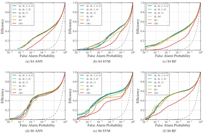
Anticipating that some of the parameters could be irrele-vant, we prepare several data sets by removing features from the list: (ρ, Δt, f, d, n). We prepare these data sets for both S4 and S6 data and run each of the classiﬁers through the training-evaluation round-robin cycles described in Sec-tion III. We evaluate their performance by computing the ROC curves, shown in Figure 1.

We note the following relative trends in the ROC curves for all classifiers. The omission of the transient’s duration, d, and the number of wavelets, n, has virtually no effect on efficiency. The ROC curves are the same to within our error, which is less than ± 1 % for our efficiency

(9)

mea-10−5 ₁₀−4 ₁₀−3 ₁₀−2 ₁₀−1 ₁₀0 False Alarm Probability

0.0 0.2 0.4 0.6 0.8 1.0 Ef ﬁcienc y (ρ,Δt,f,d,n) (ρ,Δt,f,d) (ρ,Δt,f) (ρ,Δt) (ρ) (Δt) (a) S4 ANN 10−5 ₁₀−4 ₁₀−3 ₁₀−2 ₁₀−1 ₁₀0

False Alarm Probability

0.0 0.2 0.4 0.6 0.8 1.0 Ef ﬁcienc y (ρ,Δt,f,d,n) (ρ,Δt,f,d) (ρ,Δt,f) (ρ,Δt) (ρ) (Δt) (b) S4 SVM 10−5 ₁₀−4 ₁₀−3 ₁₀−2 ₁₀−1 ₁₀0

0.0 0.2 0.4 0.6 0.8 1.0 Ef ﬁcienc y (ρ,Δt,f,d,n) (ρ,Δt,f,d) (ρ,Δt,f) (ρ,Δt) (ρ) (Δt) (c) S4 RF 10−5 ₁₀−4 ₁₀−3 ₁₀−2 ₁₀−1 ₁₀0

0.0 0.2 0.4 0.6 0.8 1.0 Ef ﬁcienc y (ρ,Δt,f,d,n) (ρ,Δt,f,d) (ρ,Δt,f) (ρ,Δt) (ρ) (Δt) (d) S6 ANN 10−5 ₁₀−4 ₁₀−3 ₁₀−2 ₁₀−1 ₁₀0

0.0 0.2 0.4 0.6 0.8 1.0 Ef ﬁcienc y (ρ,Δt,f,d,n) (ρ,Δt,f,d) (ρ,Δt,f) (ρ,Δt) (ρ) (Δt) (e) S6 SVM 10−5 ₁₀−4 ₁₀−3 ₁₀−2 ₁₀−1 ₁₀0

0.0 0.2 0.4 0.6 0.8 1.0 Ef ﬁcienc y (ρ,Δt,f,d,n) (ρ,Δt,f,d) (ρ,Δt,f) (ρ,Δt) (ρ) (Δt) (f) S6 RF

FIG. 1. Varying sample features. We expect some of the five features recorded for each auxiliary channel to be more useful than others. To quantitatively demonstrate this, we train and evaluate our classifiers using subsets of our sample data, with each subset restricting the number of auxiliary features. We observe the general trend that the significance,ρ, and time difference,Δt, are the two most important features. Between those two,ρappears to be marginally more important thanΔt. On the other hand, the central frequency,f, the duration,d, and the number of wavelet coefficients in an event,n, all appear to have very little affect on the classifiers’ performance. Importantly, our classifiers are not impaired by the presence of these superfluous features and appear to robustly reject irrelevant data without significant efficiency loss. The black dashed line represents a classifier based on random choice.

surement, based on the total number of glitch samples and the normal approximation for binomial conﬁdence interval,

P1(1−P1)/N. Omission of the frequency,f, slightly

re-duces the efficiency of SVM (Figure 1b and Figure 1e), but has no effect on either ANN or RF. A comparison between the ROC curves for (ρ, Δt), (ρ) and (Δt) data sets shows that while a transient’s significance is the most informative pa-rameter, including the time difference generally results in bet-ter overall performance. Of the three MLA classifiers, SVM seems to be the most sensitive to whether the time difference is used in addition to significance. RF, as it appears, relies pri-marily on significance, which is reflected in poor performance of the (Δt)-only ROC curves in Figure 1c and Figure 1f. The trend for ANN is not as clear. In S4 data, including timing does not change the ROC curve (Figure 1a) while in S6 data it improves it (Figure 1d). Overall, we conclude that based on these tests, most if not all the information about detected glitches is contained in the (ρ,Δt) pair. At the same time, keeping irrelevant features does not seem to have a negative effect on our classifiers’ performance.

The OVL algorithm, which we use as a benchmark, ranks and orders the auxiliary channels based on the strength of

cor-relations between transient disturbances in the auxiliary chan-nels and glitches in gravitational-wave channel. The final list of OVL channels includes only a small subset of the available auxiliary channels, 47 (of 162) in S4 data and 35 (of 250) in S6 data. The rest of the channels do not show statistically significant correlations. It is possible that these channels con-tain no useful information for glitch identification, or that one has to include correlations involving multiple channels and/or other features to exract the useful information. In the for-mer case, throwing out irrelevant channels will significantly decrease our problem’s dimensionality and may improve the classifiers’ efficiency. In the latter case, classifiers might be capable of using higher order correlations to identify classes of glitches missed by OVL.

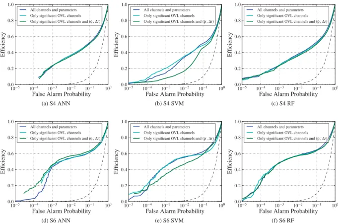
We prepare two sets of data to investigate these possibili-ties. In the ﬁrst data set, we use only the OVL auxiliary chan-nels and exclude information from all other chanchan-nels. In the second data set, we further reduce the number of dimensions by using onlyρandΔt. We apply classiﬁers to both data sets, evaluate their performance and compare it to the run over the full data set (all channels and all features). Figure 2 shows the ROC curves computed for these test runs.

(10)

10−5 ₁₀−4 ₁₀−3 ₁₀−2 ₁₀−1 ₁₀0 False Alarm Probability

0.0 0.2 0.4 0.6 0.8 1.0 Ef ﬁcienc y

All channels and parameters Only signiﬁcant OVL channels Only signiﬁcant OVL channels and (ρ,Δt)

(a) S4 ANN

10−5 ₁₀−4 ₁₀−3 ₁₀−2 ₁₀−1 ₁₀0

0.0 0.2 0.4 0.6 0.8 1.0 Ef ﬁcienc y

(b) S4 SVM

10−5 ₁₀−4 ₁₀−3 ₁₀−2 ₁₀−1 ₁₀0

0.0 0.2 0.4 0.6 0.8 1.0 Ef ﬁcienc y

(c) S4 RF

10−5 ₁₀−4 ₁₀−3 ₁₀−2 ₁₀−1 ₁₀0

0.0 0.2 0.4 0.6 0.8 1.0 Ef ﬁcienc y

(d) S6 ANN

10−5 ₁₀−4 ₁₀−3 ₁₀−2 ₁₀−1 ₁₀0

0.0 0.2 0.4 0.6 0.8 1.0 Ef ﬁcienc y

(e) S6 SVM

10−5 ₁₀−4 ₁₀−3 ₁₀−2 ₁₀−1 ₁₀0

0.0 0.2 0.4 0.6 0.8 1.0 Ef ﬁcienc y

(f) S6 RF

FIG. 2. Reducing the number of channels. One way to reduce the dimensionality of our feature space is to reduce the number of auxiliary channels used to create the feature vector. We use a subset of auxiliary channels identified by OVL as strongly correlated with glitches in the gravitational-wave channel (light blue). We notice that for the most part, there is not much efficiency loss when restricting the feature space in this way. This also means that very little information is extracted from the other auxiliary channels. The classifiers can reject extraneous channels and features without significant loss or gain of efficiency. We also restrict the feature vector to only include the significance,ρ, and the time difference,Δt, for the OVL auxiliary channels (green). Again, there is not much efficiency loss, suggesting that these are the important features and that the classifiers can robustly reject unimportant features automatically. The black dashed line represents a classifier based on random choice.

In both S4 and S6 data, the three curves for RF (Figure 2c and Figure 2f) lay on the top of each other, demonstrating that this classifier’s performance is not affected by the data reduc-tion. ANN shows slight improvement in its performance for the maximally reduced data set in the S6 data (Figure 2d), and no discernible change in the S4 data (Figure 2a). SVM ex-hibits the most variation of the three classifiers. While drop-ping the auxiliary channels not included in the OVL list has a very small effect on SVM’s ROC curve, further data reduction leads to an efficiency loss (Figure 2b and Figure 2e). Viewed together, the plots in Figure 2 imply that, on one hand, non-OVL channels can be safely dropped from the analysis, but on the other hand, the presence of these uninformative chan-nels does not reduce our classifiers’ efficiency. This is reas-suring. As previously mentioned, one would like to use these methods for real-time classification and detector diagnosis, in which case monitoring as many channels as possible allows us to identify new kinds of glitches and potential detector mal-functions. For example, an auxiliary channel that previously showed no sign of a problem may begin to witness glitches. If excluded from the analysis based on its previous irrelevance,

the classiﬁers would not be able to identify glitches witnessed by this channel or warn of a problem.

Another way in which input data may influence a classi-fier’s performance is by limiting the number of samples in the training set. Theoretically, the larger the training sets, the more accurate a classifier’s prediction. However, larger training sets come with a much higher computational cost and longer training times. In our case, the size of the glitch train-ing set is limited by the glitch rate in the gravitational-wave channel and the duration of the detector’s run. We remind the reader that we use four weeks from the S4 run from the H1 detector and one week from the S6 run from the L1 detec-tor to collect glitch samples. One would like to use shorter segments to better capture non-stationarity of the detector’s behavior. However, having too few glitch samples would not provide a classifier with enough information. Ultimately, the size of the glitch training set will have to be tuned based on the detector’s behavior. We have much more control over the size of the clean training set, which is based on completely random times when the detector was operating in the science mode. In our simulations, we start with105 clean samples,

(11)

but it might be possible to reduce this number without loss of efﬁciency, thereby speeding up classiﬁer training.

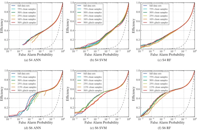
We test how the classiﬁers’ performance is affected by the size of the clean training set in a series of runs in which we gradually reduce the number of clean samples available. Runs with 100%, 75%, 50%, and 25% of the total number of clean samples available for training are supplemented by a run in which the number of clean training samples is equal to the number of glitch training samples (16% in S4 data and 2.5% in S6 data). In addition, we performed one run in which we re-duced the number of glitch training samples by half, but kept 100% of the clean training samples. While not completely exhaustive, we believe these runs provide us with enough in-formation to describe the classiﬁers’ behavior. In all of these runs, we use all available samples for evaluation, employing the round-robin procedure. Figure 3 demonstrates changes in the ROC curves due to the variation of training sets.

RF performance (Figure 3c and Figure 3f) is not affected by reduction of the clean training set in the explored range, with the only exception of the run over S6 data where size of the clean training set is to 2.5% of the original. In this case, the ROC curve shows an efﬁciency loss on the order of 5% at a false alarm probability ofP0= 10−3. Also, cutting the glitch

training set by half does not affect RF efﬁciency in either S4 or S6 data.

SVM’s performance follows very similar trends, shown in Figure 3b and Figure 3e, demonstrating robust performance against the reduction of the clean training set and suffering appreciable loss of efﬁciency only in the case of the smallest set of clean training samples. Unlike RF, SVM seems to be more sensitive to variations in size of glitch training set. The ROC curve for the 50% glitch set in S6 data drops 5%-10% in the false alarm probability region ofP0 = 10−3(Figure 3e).

However, this does not happen in the S4 run (Figure 3e). This can be explained by the fact that S4 glitch data set has ﬁve times more samples than S6 set. Even after cutting it in half, the S4 set provides better sampling than the full S6 set.

ANN is affected most severely by training set reduction (Figure 3a and Figure 3d). First, its overall performance vis-ibly degrades with the size of the clean training set, espe-cially in the S6 runs (Figure 3d). Howeer, we note that the ROC curve primarily drops near a false alarm probability of P0 = 10−3, it remains the same near P0 = 10−2 (for all

but the 2.5% set). The higherP0 value is more important in

practice because the probability of false alarm of10−2_{is still}

tolerable and, at the same time, the efﬁciency is signiﬁcantly higher than atP0 = 10−3. This means that we are likely to

operate a real-time monitor nearP0 = 10−2rather than near

10−3_{. Reducing the training sample introduces an artifact on}

ANN’s ROC curves, not seen on either RF or SVM. Here, the false alarm probability’s range decreases with the size of the clean training set. This is due to the fact that with the ANN conﬁguration parameters used in this analysis, ANN’s rank becomes more degenerate when less clean samples are available for training, meaning that multiple clean samples in the evaluation set are assigned exactly the same rank. This is in general undesirable, because a continuous, non-degenerate rank carries more information and can be more efﬁciently

in-corporated into gravitational-wave searches. The degeneracy issue of ANN and its possible solutions are treated in detail in [31].

We would like to highlight the fact that in our test runs, we use data from two different detectors and during different sci-ence runs, and that we test three very different classifiers. The common trends we observe are not the result of peculiarities in a specific data set or an algorithm. It is reasonable to expect that they reflect generic properties of the detectors’ auxiliary data as well as the MLA classifiers. Extrapolating this to fu-ture applications in advanced detectors, we find it reassuring that the classifiers, when suitably configured, are able to mon-itor large numbers of auxiliary channels while ignoring irrel-evant channels and features. Furthermore, their performance is robust against variations in the training set size. In the next sections we compare different classifiers in their bulk perfor-mance as well as in sample-by-sample predictions using the full data sets.

VI. EVALUATING AND COMPARING CLASSIFIERS’ PERFORMANCE

The most relevant measure of any glitch detection algo-rithm’s performance is its detection efﬁciency, the fraction of identiﬁed glitches,P1, at some probability of false alarm,P0.

The ROC curve is the key figure of merit and can be used to assess the algorithm’s efficiency, and objectively compare it to other methods throughout the entire range of the prob-ability of false alarm. This is useful because the upper limit for acceptable values of probability of false alarm depends on the specific application. In the problem of glitch detection in gravitational-wave data, we set this value to beP0 = 10−2,

which corresponds to 1% of true gravitational-wave transients falsely labeled as glitches. Another way to interpret this is that 1% of the clean science data are removed from searches for gravitational waves.

Our test runs, described in the previous section, demon-strate the robustness of the MLA classifiers against the pres-ence of irrelevant features in the input data. We are interested in measuring the classifiers’ efficiency in the common case where no prior information about relevance of the auxiliary channels is assumed. For this purpose, we use the full S4 and S6 data sets, including all channels with a wide selection of parameters. Using exactly the same training/evaluation sets for all our classifiers allows us to assign four ranks, (rANN, rSVM,rRF,rOVL), to every sample and compute the probabil-ity of false alarm,P0(ri)and efficiency, P1(ri)for each of

the classiﬁers. While the ranks can not be compared directly, these probabilities can. Any differences in classiﬁers’ predic-tions, in this case, are from the details and limitations of the methods themselves, and are not from the training data.

Glitch samples that are separated in time by less than a sec-ond are likely to be caused by the same auxiliary disturbance. Even if they are not, gravitational-wave transient candidates detected in a search are typically “clustered” with a time win-dow ranging from a few hundred milliseconds to a few sec-onds, depending on the length of the targeted

(12)

gravitational-10−5 ₁₀−4 ₁₀−3 ₁₀−2 ₁₀−1 ₁₀0 False Alarm Probability

0.0 0.2 0.4 0.6 0.8 1.0 Ef ﬁcienc y

full data sets 75% clean samples 50% clean samples 25% clean samples 16% clean samples 50% glitch samples (a) S4 ANN 10−5 ₁₀−4 ₁₀−3 ₁₀−2 ₁₀−1 ₁₀0

0.0 0.2 0.4 0.6 0.8 1.0 Ef ﬁcienc y

full data sets 75% clean samples 50% clean samples 25% clean samples 16% clean samples 50% glitch samples (b) S4 SVM 10−5 ₁₀−4 ₁₀−3 ₁₀−2 ₁₀−1 ₁₀0

0.0 0.2 0.4 0.6 0.8 1.0 Ef ﬁcienc y

full data sets 75% clean samples 50% clean samples 25% clean samples 16% clean samples 50% glitch samples (c) S4 RF 10−5 ₁₀−4 ₁₀−3 ₁₀−2 ₁₀−1 ₁₀0

0.0 0.2 0.4 0.6 0.8 1.0 Ef ﬁcienc y

full data sets 75% clean samples 50% clean samples 25% clean samples 2.5% clean samples 50% glitch samples (d) S6 ANN 10−5 ₁₀−4 ₁₀−3 ₁₀−2 ₁₀−1 ₁₀0

0.0 0.2 0.4 0.6 0.8 1.0 Ef ﬁcienc y

full data sets 75% clean samples 50% clean samples 25% clean samples 2.5% clean samples 50% glitch samples (e) S6 SVM 10−5 ₁₀−4 ₁₀−3 ₁₀−2 ₁₀−1 ₁₀0

0.0 0.2 0.4 0.6 0.8 1.0 Ef ﬁcienc y

full data sets 75% clean samples 50% clean samples 25% clean samples 2.5% clean samples 50% glitch samples (f) S6 RF

FIG. 3. Varying the size of training data sets. In our sample data, the number of glitches is limited by the actual glitch rate in the LIGO detectors and the length of the analysis time we use. However, we can construct as many clean samples as necessary because we sample the auxiliary channels at random times. In general, classifiers’ performance will increase with larger training data sets, but at additional computational cost. We investigate the effect of varying the size of training sets on the classifiers’ performance, and observe only small changes even when we significantly reduce the number of clean samples. We also reduce the number of glitch samples, observing that the classifiers are more sensitive to the number of glitches provided for training. This is likely due to the smaller number of total glitch samples, and reducing the number of glitches may induce a severe undersampling of feature space. The black dashed line represents a classifier based on random choice.

wave signal. Clustering implies that among all candidates within the time window, only the one with highest statistical signiﬁcance will be retained. In order to avoid double count-ing of possibly correlated glitches and to replicate conditions similar to a real-life gravitational-wave search, we apply a clustering procedure to the glitch samples, using a one second time window. In this time window, we keep the sample with the highest signiﬁcance, ρ, of the transient in gravitational-wave channel.

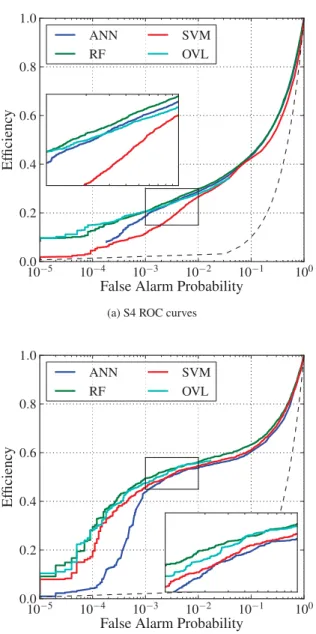
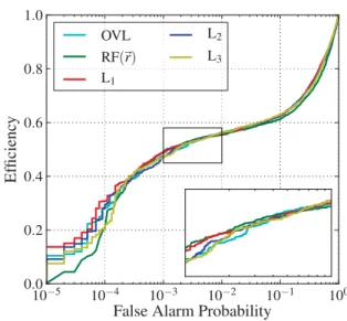
The ROC curves are computed after clustering. Figure 4 shows the ROC curves for ANN, SVM, RF and OVL for both S4 and S6 data.

All our classifiers show comparable efficiencies in the most relevant range of the probability of false alarm for practical applications (10−3_–₁₀−2_{). Of the three MLA classifiers, RF}

achieves the best efﬁciency in this range, with ANN and SVM getting very close nearP0 = 10−2. Relative to other

classi-ﬁers, SVM performs worse in the case of S4 data, and ANN’s efﬁciency drops fast atP ≤ 10−3_{. The most striking}

fea-ture on these plots is how closely the RF and the OVL curves follow each other in both S4 and S6 data (Figure 4a and Fig-ure 4b respectively). In absolute terms, the classiﬁers achieve

signiﬁcantly higher efﬁciency for S6 than for S4 data, 56% versus 30% atP0 = 10−2. We also note that the clustering

procedure has more effect on the ROC curves in S4 than in S6 data. In the former case, the efﬁciency drops by 5 - 10% (compare to the curves in Figures 3a to 3c), whereas in the latter it stays practically unchanged (compare to Figures 3d to 3f). The reason for this is not clear. In the context of detec-tor evolution, the S6 data are much more relevant for advanced detectors. At the same time, we should caution that we use just one week of data from the S6 science run and larger scale testing is required for evaluating the effect of the detector’s non-stationarity.

The ROC curves characterize the bulk performance of the classifiers, but they do not provide information about what kind of glitches are identified. To gain further insight into the distribution of glitches before and after classification, we plot cumulative histograms of the significance,ρ, in the gravitational-wave channel for glitches that remain after re-moving those detected by each of the classifiers atP0≤10−2.

We also plot a histogram of all glitches before any glitch re-moval. These histograms are shown in Figure 5. They show the effect of each classiﬁer on the distribution of glitches in the