Inattentive professional forecasters

DOCUMENT

DE TRAVAIL

N° 307

INATTENTIVE PROFESSIONAL

FORECASTERS

Philippe Andrade and Hervé Le Bihan December 2010

DIRECTION GÉNÉRALE DES ÉTUDES ET DES RELATIONS INTERNATIONALES

INATTENTIVE PROFESSIONAL

FORECASTERS

Philippe Andrade and Hervé Le Bihan December 2010

Les Documents de travail reflètent les idées personnelles de leurs auteurs et n'expriment pas nécessairement la position de la Banque de France. Ce document est disponible sur le site internet de la Banque de France « www.banque-france.fr ».

Working Papers reflect the opinions of the authors and do not necessarily express the views of the Banque de France. This document is available on the Banque de France Website “www.banque-france.fr”.

Inattentive professional forecasters

Banque de France & CREM

Herv´e Le Bihan Banque de France

December 2010

∗

We thank our discussants Bartosz Ma´ckowiak and Ernesto Past´en as well as Carlos Carvalho, Olivier Coibion, Christian Hellwig, Anil Kashyap, Noburo Kiyotaki, Juan Pablo Nicolini, Giorgio Primiceri, Sergio Rebelo, Jonathan Willis, Alexander Wolman, Michael Woodford, Tao Zha and seminar participants at the Banque de France, ECB, New-York Fed, Philadelphia Fed, San-Francisco Fed, University Paris 1 and at the conferences ESEM 2009, AFSE 2010, CESIfo on “Macroeconomics and Survey Data” and SED 2010 for useful comments. All remaining errors are ours. We are also grateful to Sylvie Tarrieu for superb research assistance as well as to Claudia Marchini and Ieva Rubene for their help with the SPF data. This paper does not reflect necessarily the views of the Banque de France. e-mails: [email protected],[email protected]

Abstract

We use the ECB Survey of Professional Forecasters to characterize the dynamics of expectations at the micro level. We find that forecasters (i) have predictable forecast errors; (ii) disagree; (iii) fail to systematically update their forecasts in the wake of new information; (iv) disagree even when updating; and (v) differ in their frequency of updating and forecast performances. We argue that these micro data facts are qualitatively in line with recent models in which expectations are formed by inattentive agents. However building and estimating an expectation model that features two types of inattention, namely sticky information à la Mankiw-Reis and noisy information à la Sims, we cannot quantitatively generate the error and disagreement that are observed in the SPF data. The rejection is mainly due to the fact that professionals relatively agree on very sluggish forecasts.

Keywords: Expectations, imperfect information, inattention, forecast errors, disagreement, business cycle

JEL Classification: D84, E3, E37

Résumé

Nous utilisons l’enquête « Survey of Professional Forecasters » conduite par la BCE, un panel trimestriel, afin de caractériser la formation des anticipations des prévisionnistes professionnels. Nous mettons en évidence plusieurs faits : (i) le caractère prévisible des erreurs de prévision; (ii) un degré significatif de désaccord entre prévisionnistes; (iii) l’absence de révision systématique : chaque trimestre, environ un quart des prévisions ne sont pas révisées; (iv) un niveau de désaccord significatif même parmi les experts qui révisent leurs prévisions (v) une hétérogénéité entre les experts du panel dans la fréquence de révision des anticipations et dans leur performance prédictive. Ces faits sont qualitativement cohérents avec les modèles théoriques reposant sur l’hypothèse d’”inattention” comme ceux de Mankiw et Reis, ou de Sims.

Dans un second temps, nous élaborons et estimons un modèle empirique qui englobe ces deux types de spécification de l’inattention. Nous obtenons toutefois que ce modèle est quantitativement rejeté : il ne permet pas de rendre compte simultanément du niveau de désaccord et du niveau de persistance de l’erreur de prévision présents dans les données. Compte tenu du degré de désaccord observé, le modèle prédit des prévisions beaucoup moins inertes que celle observées : à l’origine de ce rejet est donc un certain consensus des experts sur des prévisions inertes.

Mots-clefs: Anticipations, prévisions d’experts, information imparfaite, inattention, erreur de prévision, désaccord, cycle macroéconomique.

1

Introduction

Models in which imperfect information and the formation of expectations act as a transmission mechanism of economic fluctuations—in the spirit of Friedman (1968), Phelps (1968) and Lucas (1972)—have recently regained interest in the macroeconomic literature.1 Imperfect information has, in particular, been related to the inattention of agents to new information, a behavior that can be rationalized by costly access to information and limited processing capacities.2 One appeal of these models is to provide an alternative channel to sticky prices to explain the persistent effects of transitory shocks, and in particular monetary shocks, on the economy. Moreover, this approach can parsimoniously account for patterns of individual expectations observed in survey data that are at odds with the standard perfect information rational expectation framework, namely that forecast errors are predictable and forecasts differ across forecasters.3

In this paper, we exploit the panel dimension of such a survey of forecasts, namely the ECB Survey of Professional Forecasters (SPF), to produce new micro facts characterizing the formation of expectations. We then elaborate on those characteristics to assess whether models of inattention accurately describe the behavior of forecasters and thus may contribute to a better understanding of business cycle fluctuations. To be consistent with the recent literature we consider two types of inattention models. On the one hand, sticky information models developed by Mankiw & Reis (2002) and Reis (2006a,b) in which agents update their information set infrequently but get perfect information once they do. On the other hand noisy information models proposed by Woodford (2002), Sims (2003) and Ma´ckowiak & Wiederholt (2009) in which agents continuously update their information but have an imperfect access to it at each period.

The ECB-SPF is a quarterly panel starting in 1999 surveying around 90 forecasting units in either public or private institutions. Professional forecasters may not be representative of less sophisti-cated agents, since professionals obviously allocate substantially more time, human, collecting and computing resources to the task of forecasting macroeconomic variables. However professionals’

1_{See, among others, Woodford (2002), Hellwig & Veldkamp (2008), Angeletos & La’O (2009) and Lorenzoni (2009).}

Imperfect information is also crucial in the recent welfare analysis of information. See, among others, Morris & Shin (2002), Angeletos & Pavan (2007) or Adamor & Weill (2009). Veldkamp (2009) and Mankiw & Reis (2010) provide surveys.

2

See Mankiw & Reis (2002), Sims (2003), Reis (2006a,b) and Ma´ckowiak & Wiederholt (2009).

opinion has been shown to spread to other types of agents and therefore influence expectations and decisions of firms and households (Carroll, 2003). Furthermore we may expect professional forecasters to be the agents in the best position to pay attention to the relevant macroeconomic information. As a result, the extent of attention to news among professional forecasters can be seen as an upper bound for other agents’ attention to aggregate conditions.

We highlight five main categories of micro facts from these SPF data that we argue are consistent with professional forecasters behaving as if they were inattentive. First, the forecasts of experts exhibit predictable errors and systematic bias. Second, experts disagree as they report different predictions for the same variable at the same forecast horizon. Moreover, the disagreement between forecasters evolves over time. Third, agents do not systematically update their forecasts even when new information is released. Fourth, the forecasters who update also disagree on their forecasts. Five, the frequency of updating a forecast, the average forecast error and the revision of forecast vary across individuals.

To our knowledge, the present study is the first to document infrequent updating in survey forecasts. The originality of our approach is to exploit the fact that the European SPF provides sequences of individual forecasts for the same event (variable and date). We can therefore construct a direct micro-data estimate of the frequency of updating a forecast. The results show that, on average, each quarter, only 75% of professional forecasters do update their 1-year or 2-year forecasts while the macroeconomic environment evolves. The frequency of updating has a structural interpretation: it corresponds to the degree of attention, a key parameter in a sticky-information type of model. Furthermore, identifying forecasters that update their forecasts, we also uncover that they too disagree. Thus the lack of information updating is not the sole responsible for disagreement among experts. Even when updating their forecasts, they may not have access to the same information. This result is in line with the predictions of a noisy-information model. Lastly, the individual dimension of the data allows us to analyze the cross section distribution of the degree of attention. We find a minimum at 50% and a maximum at 100%. Moreover, the shape of the distribution reveals that the implied average inattention is not driven by a specific group of professional forecasters. We then turn to a formal empirical assessment of inattention models. More precisely, we argue that the previous results qualitatively support a model featuring two types of inattention namely

sticky-information `a la Mankiw-Reis and noisy-information `a la Sims. We therefore develop such an expectation model and then use it along with the SPF data to carry out a Minimum Distance Estimation (MDE). We find that this inattention model fails to quantitatively reproduce the ob-served persistence of the average forecasting errors together with the relatively small disagreement between forecasters. Moreover, the smoothness observed in the average SPF forecasts would re-quire a much lower attention degree than our micro data estimates. Such a low attention would in turn lead to much more disagreement than observed in the SPF data. Therefore, elements others than the mere inattention included in our expectation model are needed to reconcile both the rel-atively low disagreement among professionals and the relrel-atively high persistence of the aggregate forecasting error.

Our paper relates to the vast literature, mostly relying on US data, that studies the behavior of survey forecasts and compares it with the implications of theoretical expectation models. Numerous studies (see Pesaran & Weale, 2006 for a recent survey) found systematic aggregate forecast errors and disagreement in these data, at odds with the perfect information rational expectation frame-work. We confirm these results for a recent sample period and for European SPF data. We also complement these results by providing new empirical micro evidence on individual expectations. Our work is also related to Mankiw et al. (2003), Branch (2007), Coibion & Gorodnichenko (2008) or Patton & Timmermann (2009) who rely on the characteristics of survey expectations to assess inattention and, more generally, imperfect information theories. Mankiw et al. (2003) and Branch (2007) focus on the cross-section distribution of forecasts to calibrate the sticky-information attention parameter mentioned above. By comparison, we underline the importance of investigating the consistency of this parameter values with both the cross-section dispersion of forecasts and the aggregate forecast errors. Furthermore, we improve on their approach by considering a model which can explain the disagreement among forecasters who update their information set. Lastly, rather than calibrate it, we estimate the attention parameter using either micro-data estimates or a MDE procedure. Coibion & Gorodnichenko (2008) look at the conditional response to various structural shocks of the aggregate error and disagreement implied by surveys to disentangle the sticky-information and the noisy-information models of inattention. They find mixed support in favor of the two, as we do. The distinctive feature of our analysis is that we estimate a model

featuring simultaneously the two types of inattention. Patton & Timmermann (2009) rely on the evolution of forecasts over different forecast horizons to stress that differences in the interpretation of information, rather than different information sets are the main culprit for forecasters’ disagreement. They leave the source of these different interpretations unexplained. The model we consider is an alternative approach to generate disagreement, that does not rely on “deep” heterogeneity among forecasters.

Our paper is moreover closely linked to several recent contributions that rely on aggregate time series to estimate the attention degree in a sticky-information model of inflation dynamics (Kiley 2007, D¨opkeet al. 2008, Coibion 2010). When significant, the results imply a frequency of updating a forecast ranging from 10% to 30%, well below the figure of 75% we obtain. That we rely on a panel of professionals could explain part of the discrepancy, since these agents may update more frequently their forecasts than other types. However many of these recent studies (for instance D¨opke et al.

2008, Coibion, 2010) also use professional forecasters’ expectations to perform their estimation. The discrepancy is thus also related to the methodology. Studies that use macroeconomic time series typically rely on auxiliary assumptions on the economy and are subject to aggregation biases. By contrast, we provide a direct, arguably more reliable, micro-data estimate of this parameter that is key in sticky information models. Even if we find an attention degree that is much higher than these previous works, it still remains remarkable that professionals do not systematically update their forecasts.

Finally, our work is related to Klenow & Willis (2007) and Ma´ckowiak et al. (2009). They rely on structural models of price setting under inattention and show that several of the distinctive impli-cations of these models are supported by the dynamics of individual prices (Klenow & Willis, 2007) or sectoral price index data (Ma´ckowiaket al., 2009). By comparison, looking at the characteristics of expectations, we find more direct evidence in favor of inattention theories. We also stress some quantitative limits of the existing inattention models.

The rest of the paper is organized as follows. In section 2, we describe the European SPF data. We turn to the facts in section 3. In section 4, we develop a model of expectations that incorporate both sticky and noisy information and put it to a test. We give some concluding remarks in section 5.

2

Data: the ECB Survey of Professional Forecasters

The ECB’s survey of professional forecasters has been conducted every quarter since 1999. The survey covers around 90 institutions involved in forecasting and operating in the euro area. Each institution is asked to report, among other things, forecasts for the (year-on-year) euro area inflation rate, real GDP growth rate and unemployment rate for forecasting horizons of one year and two years.4 Respondents provide two types of forecasts. The first one is a ‘rolling forecast’, with a fixed horizon of one or two years ahead of the last available observation. The second type of forecast is a ‘calendar horizon’ forecast: in each quarter, forecasters are surveyed about their forecast for a fixed event, namely the current and next years. In this case, the forecast horizon shrinks as time goes by. At the time of the writing of this article, the last available survey round is 2010Q2, so that we have 46 time periods available. These data are matched with the corresponding realization of the forecasted variable.

The ECB SPF has been rarely used for research purposes so far. It was indeed launched with the euro and therefore was bound to cover a too short period of time for several years. However, the ECB SPF has some has some specific advantages compared to some other survey expectation data. As will be detailed below (Section 3.4.1), combining these specificities is crucial to observe the individual expectation characteristics that relate to models of inattention, in particular the ones associated with forecast revisions. To start with, the data base is a panel which implies that one can track the response of a particular individual institution over time. Moreover, the responses are quantitative rather than qualitative. By contrast, many of the survey that cover firms or households are typically repeated cross-sections, and report qualitative data.5 Furthermore, the number of actual respondents is relatively high (around 60) compared with other surveys of professional forecasters. This number is for example twice as large as the number provided in the more widely used US SPF, and leads to arguably more precise estimates of statistics based on individual expectations (the forecast average, the forecast error variance, the disagreement between forecasters, the individual probability to update a forecast). Finally, the ECB SPF provides both

4

Longer horizon forecasts are also provided but will not be emphasized here. See Bowles et al. (2007) for a thorough presentation and discussion of the survey.

5

Professionals’ forecasts relate to macroeconomic conditions whereas individual agents may be concerned with forecasting their future idiosyncratic conditions which we cannot assess here. However, in most models imperfect macroeconomic information will also have an impact on optimal individual decisions.

‘calendar’ and ‘rolling’ forecasts along with several forecast horizons, namely 4 and 8 quarters, for both of them. By contrast, the US SPF, provides only 4 quarter ‘rolling’ horizon forecasts.

We now introduce some useful notations. In the case of the rolling horizon forecasts, we denote

f_it,tx _+h individual’siforecast for the variablex at datet,hquarters ahead. The variable xis either

π(the year-on-year inflation rate), ∆y(the year on year GDP growth rate) oru(the unemployment rate). The forecast horizon h is set to 4 or 8 quarters ahead of the last observation of variable x

available at the date of the response to the survey. Importantly there is an observation lag, τx, between the date of the response to the surveytand the date of the last publicly released figure of each macro variable, t−τx+h. The observation lag varies across variables: inflation is observed with a one month lag, unemployment with a two month lag and GDP growth with a two quarter lag. The survey thus actually collects:

f_it,tx −τx+h.

In practice the SPF reports data for h= 4 or h = 8. For notation simplicity, in the following, we drop the reference to the observation lag and simply refer to f_it,tx _+h.

For the calendar horizon case, the forecast horizon is either the current or the next calendar year. The horizon is not adjusted for information lag. Letting T be the last quarter of a calendar year in the sample, calendar horizon forecast can be written as

f_it,Tx =f_it,tx _+(T−t)

The second term in the equality makes clear that, for each year in the sample, the forecast horizon

T−tdecreases with t. For notation simplicity again, we use the notationf_it,Tx .

Let xt+h be the realization of the forecasted variable at date t, we denote exit,t+h individual’s i forecast error at date t+h, namelyex_it,t+h =xt+h−f_it,tx _+h.6 The average forecast error is defined by ex_t,t+h = _n1

t

Pnt

i exit,t+h, with nt the number of respondents to the survey at date t. It can alternatively be defined with reference to the average, or consensus forecast,f_t,tx_+h= _n1

t

Pnt

i fit,tx +h simply through the equality ex_t,t+h=xt+h−ft,tx+h.

6

For rolling forecasts, the date of the realization takes into account the observation lagτx mentioned above in

3

Some facts about individuals’ expectations

3.1 Fact 1: Forecasters are biased

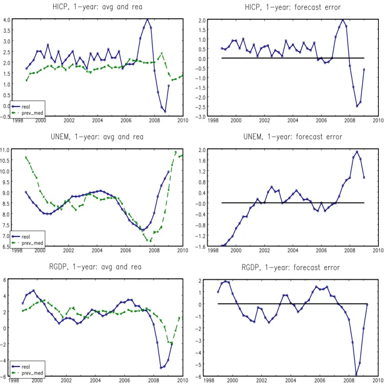
The professional forecasters make, on average, predictable errors. This emerges from Figure (1) which shows, in the left panel, the time series of the so-called consensus forecast for the 1-year hori-zon7together with the realizations of the predicted variable, and, in the right panel, the time-series of the corresponding average forecast error. It is striking to see that periods of under/overestimation of the target variable realizations are very persistent, and last for more than 1 year,i.e. over time periods that are longer than the forecast horizon.8

Table (1) further asserts these points by providing descriptive statistics on realizations, average fore-casts and errors and a test on the predictability of forecast errors. Inflation has been underestimated by an average of .56% (on an annual rate). Real GDP growth has been overrated by an average of .27%, mainly due to the recent crisis. Finally unemployment exhibits a small underestimation of about .04% over the period. These systematic biases explain why the root-mean-squared-error of the forecasts is larger than the variance of the forecasted series.

Systematic biases go along with very persistent forecast errors. Their first order auto-correlations range from .735 for inflation to .860 for unemployment.9 The bottom panel of Table (1) also shows the result of a regression of the average forecast error on the last error known at the date when the forecast was made (that is h quarters before, with h = 4). For the three variables (inflation, unemployment and output), the coefficients significantly differ from zero. Thus, errors are predictable on the basis of the information set available at the date of forecast. These results confirm other references on the topic.10

Relationship with models of information rigidity Predictable forecast errors are a

predic-tion of bothsticky information andnoisy information inattention models. Forecasters are rational

7

The consensus is defined as the average of individual forecasts for each date in the sample. The median forecast across forecasters is very close to this average.

8

This is strikingly the case for inflation with a systematic average underestimation up to 2006.

9_{These differences in forecasting performances do not seem to be related to differences in the average number of}

respondents, which are broadly the same for all three variables.

10

but exhibit biased average forecasts because they have an imperfect information on the current state of the economy.

More precisely, in a sticky information model, agents update their information set infrequently with a probability of updating given and constant across dates and individuals. Therefore, each date, only a fraction of the population has access to the last vintage of macroeconomic news. The average forecast is therefore partly made of individual forecasts that are predictable with respect to the new information set.

In a noisy information model agents update their information but they know that the news they get is imperfect and therefore only partly pass it onto their forecast. The average forecast thus incorporates only part of this new information, which makes the forecast error predictable with respect to the (perfect) information available.11

In the following sections we exploit the panel dimension of the data set to document two other characteristics of individual forecasts that these approaches imply: disagreement and inattention.

3.2 Fact 2: Forecasters disagree

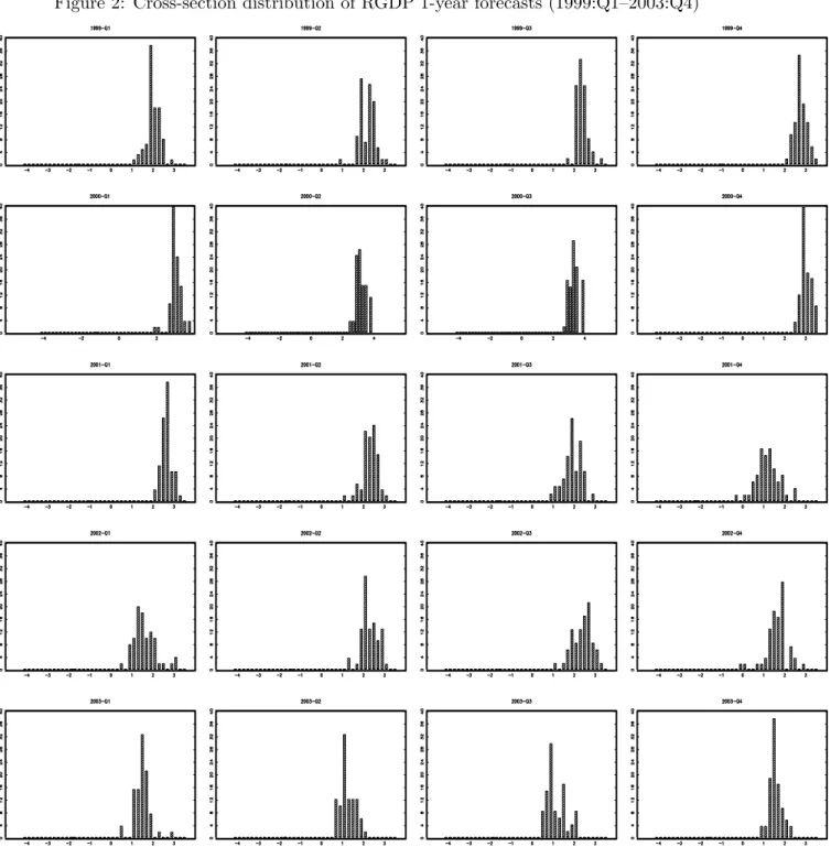
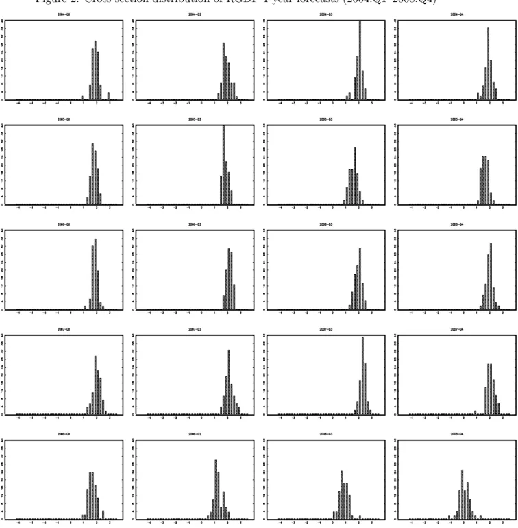
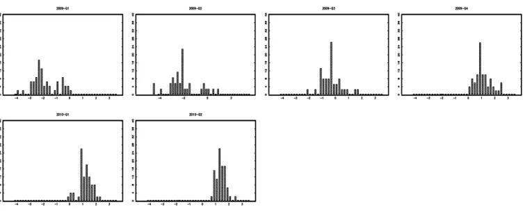
A second pattern in the data is that forecasts differ among forecasters even though they forecast the same object. This is illustrated in Figure (2) which plots the sequence of cross-section distributions of 1-year forecasts for all survey vintages in the sample.12 The distribution never degenerates to a single peak, which illustrates that disagreement is present at any date. The result is particularly striking given that forecasters in our sample are experts who presumably have access to the same information set.

An empirical assessment of the extent of disagreement among forecasters is usually done by calcu-lating the cross-section standard deviation of forecasts at each date,σ_tx, namely, using the notations introduced in the previous section

σx_t,h = " 1 nt nt X i=1 f_it,tx _+h−f_t,tx_+h2 #1/2 . 11

Here it is implicitly assumed that the econometrician can have access ex-post to perfect macroeconomic informa-tion.

12

To save space, we only present the distribution of individual forecasts for real GDP growth but qualitatively similar results hold for either unemployment or inflation forecasts.

Table (3) reports the time average disagreement, σ_hx, for the 1-year horizon rolling forecasts. This average disagreement is equal to .26 for inflation, .26 for unemployment and .33 for real GDP (see Table 3). Expressing these values as a fraction of the underlying variable standard deviation over time we obtain a normalized indicator of disagreement of 42%, 43% and 31% for, respectively, inflation, unemployment and real GDP.

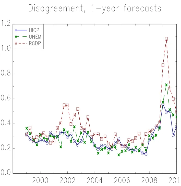
Figure (3) shows the time series of disagreement, σ_t,hx , for the 1-year horizon rolling forecasts of the three macroeconomic variables of interest. Disagreement across forecasters is not constant over time and the three time-series of disagreement have a strong positive correlation.13

It is worth investigating whether this disagreement is completely random—and in particular repre-sents measurement errors only—or whether it stems from information imperfections, for instance a slow diffusion of macroeconomic news among forecasters. In that second case, the cross-section distribution of forecasts would spread out after the shocks and then narrow to a new average level. This phenomenon seems consistent with a crude event study applied to the sequence of forecasts’ histograms of Figure (2). Consider for instance the episode of the cyclical downturn of 2001. The distribution of growth forecasts, which was very concentrated around 3%, spreads out toward zero leading to a larger dispersion. Then the distribution narrows again over 2002 and 2003 but around a lower average of about 2%. Even clearer is the impact of the current recession (years 2008-2009): along with the recession, the support of the distribution of forecasts widens substantially to the left, and several local modes appear.

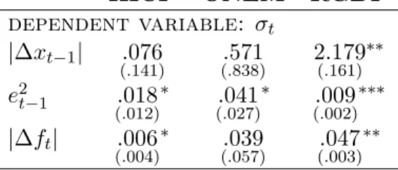
We go further in investigating the link between disagreement and economic news using formal statistical tests. More precisely, we regress disagreement at timet,σx

t,h, on several rough measures of shocks hitting the economy: the last absolute variation in the forecasted variable, |∆xt−1|,

the squared last forecast error, (ex

t−1,t+h−1)2, and the current absolute change of the forecast,

|∆f_t,tx_+h|= f x t,t+h−ftx−1,t+h−1

. Results are presented in Table (2) and show that the coefficients are all positive and most of them are significant: disagreement is an increasing function of the amplitude of the shocks hitting the economy.

This last evidence somehow contrasts with Coibion & Gorodnichenko (2008) who find that the

13

Relying on rolling-horizon forecasts to evaluate forecasters’ disagreement is important to avoid the seasonal patterns emerging from the resolution of uncertainty as time gets closer to the forecasted event one gets when relying on calendar-horizon forecasts instead.

dispersion of inflation forecasts does not react to structural shocks. They however also recognize that the results are sometimes mixed and seem to come from the fact that these structural shocks only account for small fractions of inflation total time variance.14 By contrast, here we analyze the unconditional reaction to a mixture of all events that can shock the economy and find that the information implying a change in the level of forecast takes time to spread out among agents.

Relationship with models of information rigidity The results that forecasters disagree and

that the extent of disagreement varies over time can be rationalized by both sticky-information

or noisy-information models of expectations. In both cases, disagreement is a consequence of imperfect information which implies that agents do not have the same information set.

In asticky-information model, when a large shock hits the economy, individuals who update their information set produce forecasts which are quantitatively very different from individuals who do not. These differences are less pronounced in the wake of a small shock. Consequently, the extent of disagreement evolves with the magnitude of the shocks hitting the economy.

In a noisy-information setup, forecasters think differently because they randomly get different perception of reality. In simple versions of this approach, and by contrast with simple sticky-informationmodels, disagreement does not change with the size of the shocks hitting the economy.15 In these setups, disagreement is initiated by the realizations of the idiosyncratic noise that prevent individuals from perfectly observing the true state of nature and that are assumed to have a variance that is constant over time and across individuals. The disagreement is thus not affected by the size of the macroeconomic shocks hitting the economy. It is however possible to refine this simple version of a noisy information model such as to generate time-varying disagreement also in this setup. This would be the case if, for instance, one introduced conditional time variance of the noisy signal correlated with the size of the true shock, or heterogeneity in the noise among the population of forecasters so that the ones that monitor the shock the best disagree more with the ones that have very imprecise signals after a big shock than after a small one.

14

Among the several structural shocks they investigate, none account for more 35% of total inflation variance, even in the long-run. Moreover, depending on the horizon, the share of total variance that these shocks altogether cannot account for ranges from 67% to 47% (see Section 5.2 and Appendix C in their paper).

All in all, predictable and biased forecasts errors and disagreement among forecasters suggest that both sticky information and the noisy information models may be good candidates to understand and describe how expectations are formed.

The next three subsections go further by documenting other patterns in the SPF data, that are related to the unfrequent updating of forecasts and, as we argue below, can be related to the inattention of professional forecasters.

3.3 Fact 3: Forecasters do not systematically revise their forecasts

To our knowledge, it is an original contribution of the present paper to document the attention of professional using individual data. While average forecast errors can be constructed using data on the average or consensus forecast, and time-specific disagreement can be assessed using data sets of repeated cross-sections, our measure of the degree of attention can be built only owing to the panel data structure of the SPF data set (at least two forecast sets must be observed for each individual). In this section, we first describe this measure, then turn to the results we obtain on our sample, and finally discuss the robustness of our indicator.

3.3.1 Measuring the degree of attention

The panel dimension of the SPF data set allows us to build different measures of the average frequency with which an individual revises its forecasts over time. This frequency of updating a forecast provides a measure of the extent with which agents pay attention to new macroeconomic information by incorporating it in their forecasts. It corresponds to a structural parameter insticky information models, called the degree of attention, i.e. the frequency with which agents update their information set and therefore, in these models, their forecasts.

More precisely, we consider the quarterly probability of revising theh-step ahead forecast between datet−1 andt. Lettingf_it,tx _+h be individual’siforecasth quarters ahead for variablex at time t, the probability we aim at estimating is

λx_it(h) =P(f_it,tx _+h6=f_itx_−1,t+h).

empirical counterparts to this attention degree using the SPF data.

Our first indicator relies on calendar horizon forecasts. At all dates, each forecaster is surveyed about a given calendar year. Recalling that T is the index of the last quarter of a given calendar year in the sample, the survey brings information on the probability of revision on a quarterly basis given by

λ_tx(T−t) =P(f_it,Tx 6=f_itx−1,T).

In practice the ECB-SPF surveys forecasters about their expectations for the current calendar and the next calendar years, as well as, in the third and fourth quarter vintage of the survey, about their expectations for two years ahead. Therefore, for each calendar year, sayY, ending in quarterT, we have a sequence of 10 forecasts: two sets of forecasts made at the third and the fourth quarters of yearY −2, and 8 sets from the first quarter of yearY −1 onwards. Thus we can build a sequence of 9 forecasts revisions, for the same event T, and forecast horizons h = T −t = 1, . . . ,9. The degree of attentiveness for the calendar year ending inT and the horizonh can be estimated using the empirical frequency

b λx_t,cal(h) = 1 nt nt X i=1 I(f_it,Tx 6=f_itx−1,T),

withh=T−t= 1,· · ·,9,ntthe number of respondents to the survey at datetandI(f_it,Tx 6=f_itx−1,T) an indicator function equal to 1 if fx

it,T 6=fitx−1,T and 0 otherwise.

A second measure of the probability to update a forecast can be derived from rolling horizon forecasts, exploiting the fact that they are provided for both a 4-quarter and a 8-quarter horizons. Consider the 8-quarter horizon forecast released at date t−4 by forecaster i, f_itx_−4,t+4. This can be compared to the 4-quarter horizon forecast released 4 quarters later f_it,tx ₊₄ so as to define the probability of a updating on a yearly basis

λx_t,rol(4) =P(f_it,tx ₊₄6=f_itx_−4,t+4).

An empirical estimate is obtained using b λx_t,rol= 1 nt nt X i=1 I(f_it,tx ₊₄ 6=f_itx−4,t+4),

withI(f_it,tx ₊₄6=f_itx_−4,t+4) an indicator function equal to 1 iff_it,tx ₊₄6=f_itx_−4,t+4 and 0 otherwise. By contrast with the previous measure, the horizon is bound to 4 quarters due to data limitations. We therefore skip the horizon index in the notation, referring to bλx_t,rol =bλx_t,rol(4).

This probability to update compares two forecasts that are 4 quarters away from each other. It can be converted to a quarterly adjustment rate, bλx_t,rol,q if one assumes that the probability of not updating is constant over the 4 quarters. In that case, the probability of not updating over the whole year is (1−λx_t(4)) = (1−λx_t(1))4 so that a quarterly attention rate estimate is b

λx_t,rol,q = [1−(1−λbx_t,rol)

1 4]

Furthermore, assumingλx_t(h) is constant over time and across horizons, we can also recover micro-data based estimates of the average attention degrees λbx_cal and bλx_rol,q by simply taking the time average of the empirical frequencies defined above. These estimates can be compared with the macro-data estimates of Kiley (2007), Coibion (2010), D¨opkeet al. (2008) or calibration in Mankiw

et al. (2003). In addition to assuming a constant attention degree, these previous works also needed auxiliary macroeconomic assumptions, such as the price-setting behavior of firms, to achieve their estimation. By contrast we provide a more direct estimate based on micro data.

Interpretation of λx_t(h) as a measure of attention deserves further discussion. It could in theory be the case that a forecaster chooses not to revise his forecast in spite of having updated his information set. However, given the vast information set available to professional forecasters we deem unlikely that updating the information set leads to an exactly unchanged optimal forecast after one quarter. Rather, those cases more plausibly correspond to cases where either the forecaster chooses not to run a new forecast exercise, i.e. not to pay the cost of processing the new information by running a full statistical exercise, or not to pay the cost of communicating the new information within or outside the institution. In both situations, the forecaster chooses to leave his public forecast unchanged because of information cost. It is therefore relevant to characterize this lack of reaction to news as (optimal) inattention.16

3.3.2 Results

The first result is that the estimated attention degree is lower than 100%: forecasters do not update systematically their forecasts on a quarterly basis. This can be seen from Figure (4) which

16

Alvarez, Lippi & Paciello (2010) describe a model where firms pay an information cost to calculate the optimal reset price (i.e. implement a price review) and then decide to pay or not the usual menu cost of changing the price. Here the forecaster could be seen as paying the price to calculate the optimal forecast but not the one to change the optimal forecast because of the cost of communicating the reasons of this change.

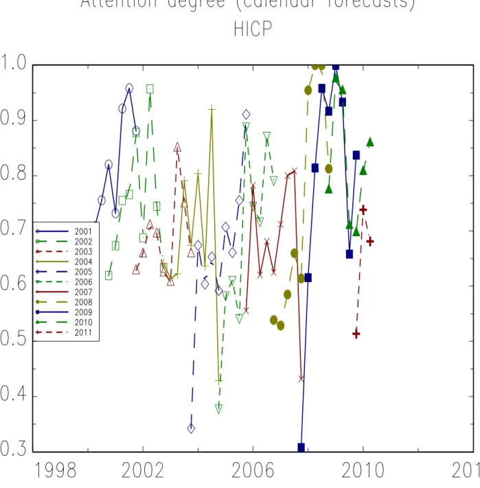
presents the estimate of attentionbλx_t,cal(h) for the HICP variable. Figures for real GDP growth and unemployment are not reported to save space but have a similar pattern. Each line in the figure reports a sequence of forecast pertaining to the same calendar year TY. There are thus 11 lines corresponding to calendar horizons from Y = 2001 to 2011. At each point in time, t, bλπ_t,cal(h) is the proportion of forecasters revising their forecast for a given target calendar yearTY ending with quarter T. The associated forecasting horizon is thus h = T −t. Sequences of forecast revisions partially overlap since, in each vintage of the survey, respondents are asked their forecast for both current and next calendar year.

Although attention is not complete, with a probability of forecast revision varying between 60% and 100% depending on the date, t, it is much higher than the values provided by previous empirical studies. Table (3) shows that the averageλbx_cal across horizons and dates is 71% for HICP, 74% for the unemployment rate and 80% for GDP growth. Averaging across variables the typical degree of attention is thusbλ_cal'75%. By comparison, Mankiw et al. (2003) calibrated a value ofλb= 10% for monthly data, i.e. a corresponding bλ= 27% when converted to quarterly data, to reproduce the disagreement in US-SPF inflation rate forecasts.

A second result that stands out from our estimation is that the average probability to revise a forecast increases when the forecast horizon decreases: all lines in Figure (4) are upward sloping. Two factors can explain this pattern: first, mean reversion implies that long run forecasts are close to the unconditional average of the process. So that news that lead to revising short run forecast may leave the forecast at a long horizon unchanged. Second, it may be the case that forecasters put more attention on revising their forecast for closest forecast horizons. Experiments in the next section suggest both factors are present.

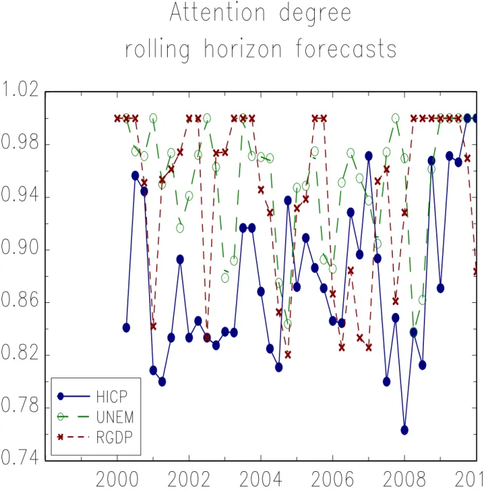
A third pattern is that the average attention level varies over time. This can be seen from the average level of each curves in Figure (4) but is even clearer when one looks at Figure (5) which plots the evolution of the alternative attention indicator bλx_t,rol, over time for the forecasts of the three variables x and shows that there is a significant degree of fluctuations in these parameter. A fourth and last result stemming from the bλx_t,rol estimate is that forecasters do not update sys-tematically their forecasts even on a yearly basis. This confirm our first result that attention is not equal to 100% when looking at bλx_t,cal(h) estimates. It is somewhat even more striking since

here some forecasters choose not updating their one-year ahead forecast even after having learned one year of macroeconomic news. Table (3) reports the time average attention degree,λbx_rol for the three macroeconomic variables x in the sample. It is equal to respectively 88% for inflation, 95% for unemployment and 94% for GDP. Converting these average probability of forecast revision to quarterly figures gives frequencies,bλx_rol,q, of 41%, 53% and 51%. Averaging across variables x one getsbλ_rol,q '48%. The difference between this result and the averagebλ_cal '75% is further evidence that the frequency of updating is not constant over forecast horizons. Our assessment is that bλ_cal is the most reliable indicator. Indeed, in practice, 8-quarter rolling horizon forecasts are usually not a conventional exercise implemented by professionals. Moreover, since calendar forecasts are available for adjacent quarters, it is more likely that they compare forecasts delivered by the same forecaster.

Relationship with models of information rigidity That forecasters do not update their

fore-casts at each period is a prediction ofsticky-information models of expectations. In this approach, agents updating their information systematically also update their forecasts so that not revising a forecast is equivalent to not revising information.17 On the contrary, the presence of non-updating in the data is not a direct consequence ofnoisy-information models. Individuals receive an imper-fect signal on the true state of the economy, but at each period they try to infer this imperimper-fectly observed state incorporating the news they received. Forecasts are thus revised at each period. Our results also show that the attention degree varies over time. By contrast, the sticky information model of Mankiw & Reis (2002) postulates that λis constant. Observing fluctuations in aggregate attention is not a direct evidence against the sticky information model of Mankiw-Reis. Indeed it could be reconciled with the more general model of inattention proposed by Reis (2006a) which, under some restrictions, aggregates to a Mankiw-Reis model in which inattention can be described by a single parameter. Note however that also we find a degree of attention that also varies with the forecasting horizon as shown in Figure (6) which violates these conditions of aggregation.

17

A more stringent prediction of these models is that the full stream of future forecasts is unchanged when a forecaster does not update his information set. However, this model does not predict that a forecaster may only revise part of this stream, so that revising a forecast for a particular horizon implies revising for the whole stream.

3.3.3 The influence of rounding

Almost all forecasts (97% of forecast figures) in our data set are reported with one digit only. Failure to revise a forecast may thus merely reflect the fact that these institutions report only rounded figures.

Rounding in our context can be interpreted in two different ways. First, one can consider rounding as a form of inattention. Indeed it is not formally requested by the ECB SPF questionnaire that figures are provided with a single digit, so providing rounded figures may reflect the cost of pro-cessing and communicating the information discussed above. Under an alternative interpretation, there is widespread acknowledgement that higher order digits are not economically meaningful, or the forecasters expect that a rounded figure is requested by the survey. Rounding would then lead to underestimate the degree of attention.

To obtain a quantitative assessment of the influence of rounding on our estimation results, we perform the following experiment. We use an estimated VAR model as a simulation and forecasting device, drawing shocks from a multivariate distribution with a covariance matrix equal to that of the estimated innovations.18 We start by simulating a large sample of artificial observations of length S using this VAR model (S = 2000). We then generate a number S of recursive sets of forecasts, up to a 12 quarter horizon, for each date in the simulated data set. Consistently with the way figures are reported in the SPF survey, we aggregate forecasts for quarterly inflation and GDP growth into forecast for annual year-on-year growth rates. We then round each forecast to the first digit. Using the data set of rounded forecasts, we compute the probability that two adjacent forecasts, corresponding to the same forecast horizon (i.e. the same target date) are different. We are able to compute such a quarterly frequency of forecast revision for all horizons h = 1 to

h = 9. Crucially, in our simulation exercise, inattention is absent from the forecasting model: actual forecasts are updated every period in line with the VAR model. As a result, the probability of not updating the forecast is here an estimate of the bias to our measurement of attention that is due to rounding. The magnitude of this bias will obviously depend on several parameters of the exercise: the horizon considered (we expect more bias at longer horizons due to mean reversion), the size of the innovation variance (larger shock will imply lower bias since forecast revision will

18

be too large to be wiped out by rounding) and the persistence of the process (low persistence of shocks will imply fast mean reversion thus less forecast revision).

The results for inflation are plotted in Figure (6). The estimated probability of updating a forecast is 83% for the horizon h = 9 quarters and rises to 91% for the horizon h = 1. These figures are lower than one, which suggest there is actually a rounding bias. The probability also increases when the target date gets closer, rationalizing the pattern of Figure (4). However these figures are at all horizons markedly above the estimates of attention we recover from actual SPF micro data, as seen in Figure (6) for the calendar forecast revision case. Thus, independently of rounding effects, there is a degree of supplementary inattention in professional forecasts.

3.4 Fact 4: Forecasters who revise disagree

The panel data set allows us to observe at each date the number of forecasters updating their forecast. We further exploit this specificity of the database in order to document the behavior of the forecasters when they update their forecasts.

We computed at each date in the sample the disagreement among forecasters that do revise their forecast. To get a sense of its importance, we compare it with the disagreement among all forecast-ers. Figure (7) gives a scatter plot of the level of disagreement in the whole population of forecasters on the x axis against disagreement among the set of forecasters that have revised their forecast at the same date on the y axis. Each observation in the plot corresponds thus to one date and one variable. They are all close to the 45 degree line. The correlation between the two disagreements is thus strongly positive, as high as 97%. At each period, the overall level of disagreement is very similar to the level of disagreement among revisers.

We also investigate whether forecasters update forecasts for several macroeconomic variables at the same time or balance their updating across dates and variables. More precisely we compute (over all observations) and for each variable (inflation, GDP growth, unemployment) the probability that the forecast of this variable is revised, conditional on the fact that the forecast of another variable (inflation, GDP growth, unemployment) has been itself revised. Figures are reported in the bottom panel of Table (3). The notion of forecast revision considered here is the rolling horizon forecast (not converted to quarterly figures). Figures for the conditional probability of revision range from

0.877 (probability of revising inflation forecast given that unemployment forecast was changed) to 0.951 (probability of revising unemployment forecast given that inflation forecast was changed). Recalling that the unconditional probability of forecast revision range from 0.88 (for inflation) to 0.95 (for unemployment), the probability of revising a forecast is thus of the same order whenever forecasts of other variables have been revised.

Relationship with models of information rigidity A prediction ofsticky-informationmodels

is that forecasters who revise their information set will draw the same optimal forecast and thus should not disagree. Therefore this approach cannot explain the large degree of disagreement among forecasters updating their forecast we find. By contrast, noisy-information models can generate disagreement between forecasters who revise since every of them has a specific information due to the heterogenous signals on the true state they receive.

In both approaches, the inattention can be rationalized by resorting to the assumptions of limited computational capacity or costly information. In this logic of rational inattention, forecasters could face a trade-off in the degree of attention devoted to the alternative variables. The strong positive correlation at the individual level between the forecast revisions of the different variables shows this is not the case. Once a forecaster update his information set, he tends to update his forecasts of every macroeconomic variable.

3.5 Fact 5: Forecasters are heterogeneous

The SPF data set finally allows to investigate the cross-section properties of individual forecasts. We find that forecasters are heterogenous in terms of their average forecast error, their average attention degree and their average forecast revision.

We first look at individual average forecast errors, namely

ex_i,h= 1 Ti Ti X t=1 ex_it,t+h,

with Ti the number of forecast observations available for individual i. The top panel in Figure (8) reports the cross section distribution of these individual average bias for 1-year ahead rolling inflation forecasts. On average, professionals underestimated the inflation rate but some of them

were more optimistic and some others were more pessimistic. There is thus a systematic pattern in disagreement since the average forecast bias differs across experts, with substantial dispersion between individuals. The individual average bias ranges broadly from -1% to 1%.19 The histogram also enlightens that disagreement does not come from some outlier professionals.

We also compute a measure of the attention degree for each individual forecaster. To do so, we assume an attention degree λx_it(h) = P(f_it,tx _+h 6= f_itx_−1,t+h) that is homogenous across dates t,

λx_it(h) =λx_i(h). We can then estimate this individual specific attention degree as the percentage of quarters in which his forecasts for a given horizonh are being revised,

b λx_i(h) = 1 Ti Ti X t=1 I(f_it,tx _+h 6=f_itx−1,t+h).

The middle panel of Figure (8) plots the cross-section distribution of λx_i(h) for the 1-year rolling inflation forecasts. The conclusion is that the degree of attention varies across forecasters. Though there is a mass of forecasters with values of λi above 80%, the dispersion is substantial. The less attentive among forecasters revise on average their forecasts every 2 quarters while the most attentive ones adjust every quarter.20

Moreover, as a measure of the extent of forecast revision, we also calculate the average absolute of forecast revision between two subsequent quarters at the individual level

|∆f_i,hx |= 1 Ti Ti X t=1 f_it,tx _+h−f_itx−1,t+h .

The cross-section distribution of the average revision for the 1-year rolling inflation forecasts is depicted in the bottom panel of Figure (8), underlining again substantial heterogeneity around a mode of .28%.

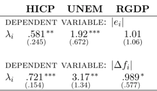
Finally, we investigate whether differences in the individual attention degree generate differences in both the individual average forecast errors and revisions. We regress the absolute value of the individual average forecast error,|ex_i,h|, and of individual average forecast revision,|(∆f_i,hx )|, on the individual attention rate, λx_i(h). Table (4) provides the results for the 1-year rolling forecasts of

19_{This systematic disagreement pattern can be linked to disagreement stemming from heterogeneity in priors or in}

models as Patton & Timmermann (2010) put forth.

20

The fact that some forecasters systematically adjust their forecasts also shows that rounding is not the mere responsible for observing a frequency of forecast revision lower than one. Would it be the case, no forecaster would systematically update.

inflation, unemployment and real GDP. Strikingly, attention is positively correlated with forecast errors and forecast revisions.

Relationship with models of information rigidity The cross-section heterogeneity observed

in average individual forecast errors can be generated both by sticky-information and noisy-information models, postulating that agents have either different frequencies of updating their forecasts or different precisions in their noisy signals. This heterogeneity could be rationalized by resorting to different information capacities constraints. However neither model generates system-atic forecast bias so that the unconditional individual average errors should be zero. The observed non-zero average forecast errors can only be associated with non-zero in-sample bias due to the particular history of news over the time sample studied.

Again, onlysticky-information models generate a lack of systematic forecast revision. Postulating heterogeneity in the frequency of updating has the potential to rationalize the heterogeneity in forecast errors that is also observed. Allowing for heterogeneity in the frequency of updating the information set may give rise to an aggregation issue. The frequency of updating the information that is consistent with the pattern of the average forecast across the whole population of hetero-geneous forecasters would be lower than the average of the individual probability of updating (see Carvalho, 2006).

Finally, both sticky-information and noisy-information models can generate heterogeneity in the cross-section of the average size of forecast revisions. In thesticky-information setup, this revision will decrease with the degree of attention. When forecasters update more frequently their informa-tion set, they incorporate more frequently the news in their forecast and therefore are subject to a lower probability of a large revision in the future. This is at odds with the results of Table (4). By contrast, in the noisy-information framework and for low attention level, i.e. very noisy indi-vidual signals, the forecast revision can become an increasing function of inattention. Very noisy signals produce almost no updating of forecasts because forecasters know about their imprecision. However, this property of the model does not help explain why the frequency of revision increases the size of the forecast error and the forecast revisions. These results could hint to a situation where the causal link is reversed: attention increases when forecasters had bad previous forecast

performances implying large forecast errors and forecast revisions.

4

Models of inattention: a quantitative assessment

The previous section has shown that the SPF data features the two basics ingredients that are in line with either a sticky information model of expectations`a laMankiw-Reis or a noisy information model`a la Sims: biased forecasts and disagreement among forecasters. Moreover, forecasts are not always updated, a prediction of Mankiw-Reis’ model and agents disagree on their forecasts even when they update their information/prediction, a prediction of Sims’ model. These qualitative

results suggest a model of expectations in which both type of inattention coexist: agents infrequently update their information set and when do they get a noisy perception of the true information.21 In this section we develop such a model of individual expectation and then assess wether it is able to

quantitatively match the average forecast errors, disagreement and probability to update a forecast that we observe in the data using a formal testing procedure.22

4.1 A sticky and noisy information model

4.1.1 DGP and information structure

We assume that the economy can be described by the following reduced form VAR(p) model

A(L)Xt=t, t∈Z,

where Xt is a set of n macroeconomic variables, centered on their average, L is the lag op-erator, A(L) ≡ Pp_k=0AkLk has all its roots outside the unit-circle and A0 = I and where

E{t|Xt−1, . . . , Xt−p} = 0. The VAR(p) model can be rewritten in the usual more compact first-order VAR companion form

Zt=F Zt−1+ηt,

21

This approach shares some features with the price-setting model of Woodford (2009). In this setup, firms have to choose on implementing a price review knowing that they will get a noisy information on the true state of the economy. This leads to optimal non-systematic price review and, when it happens, to reset prices that are determined conditional on the noisy information.

22_{Given that we do not have a clear-cut interpretation of what lies behind the heterogeneity of forecasters we}

withZt= (Xt0 Xt0−1· · · Xt0−p+1)0 and ηt= (0t 0· · · 0)0.

Letibe an individual in the population of forecasters, i= 1, . . . , n. At each date, every forecaster may update his information set or not. Along the lines of Mankiw & Reis (2002), we model this updating as a Poisson random variable, P(λ). Therefore λ is the probability to update and pay attention to the news. It is also called the degree of attention. Assuming that the population of forecasters is large, by the law of large numbers, each date t a fraction λ of the total population updates its forecast. Consequently, at each point in time, the whole population of forecasters is split into groups, generations say, within which each forecaster refers to the same vintage of information. We let j denote the generation of forecasters that last updated their information set

j periods before the current one,i.e. int−j. Thusj is also an index of the vintage of information they use. The fraction of generation j in the whole population is given by λ(1−λ)j. In Mankiw & Reis (2002) model, every agent updating his information set gets a perfect signal on the state of the economy Zt. The optimal forecast at horizonh is given by the expectation conditional on this perfect information, E(Zt+h|Zt) = FhZt. It is therefore identical for every forecaster who updates. Likewise, the forecasters who last updated in t−j receive a perfect signal on Zt−j and their optimal forecast for t+h is the conditional expectation with respect to that information vintage, E(Zt+h|Zt−j) =Fh+jZt−j. So, the Mankiw & Reis (2002) information structure implies no disagreement within a generationj of forecasters. As the previous section made clear, this is at odds with the facts.

We therefore extend Mankiw and Reis’ model to include imperfect perception of the information when updating. More precisely, we assume that, when an agent iupdates his information, he gets a noisy perception of the true state, Zt, namely a signal Yit that follows

Yit=H0Zt+vit, vit∼iid(0,Σv),

whereH is a matrix that selects the state variables that are observed with a noise.23 Remark that the average over forecasters gives the right signal: Ei(Yit) = H0Zt. A simple way to rationalize this noise is to rely on the fact that forecasters use real-time data which they know are prone to measurement errors.

23

A typical case isH=I, in which case forecasters have noisy perceptions of all the state variables. An alternative would be to consider that forecasters have perfect access to past realizations ofXt.

4.1.2 Optimal individual forecasts

Letfit,t+h denotes agent’sioptimal forecast for the vectorX at datet+h, with respect to datet information (andf_it,tx _+h the corresponding expectation for the specific component xin X). Every individual updating his information set faces the problem of inferring the true state of the economy,

Zt, from his imperfect signal Yit. Let Zit|t denotes the date t state of the economy perceived by agentiat date t: Z_it|t= E(Zt|Yit, Yit−1, . . .). Its optimal vector of forecast is given by

fit,t+h = E(Zt+h|Zit|t) =FhZit|t.

A solution to this signal extraction problem is given by the Kalman filter namely,

Zit|t=Zit|t−1+Git Yit−H0Zit|t−1

,

withZit|t−1= E(Zt|Yit−1, Yit−2, . . .) =F Zit−1|t−1, andGit the gain of the Kalman filter, defined by

Git=Pit|t−1H H0Pit|t−1H+ Σv

−1

,

wherePit|t−1 denotes the variance of the perceived forecast error,

Pit|t−1 = E

(Zt−Zit|t−1)(Zt−Zit|t−1)0

.

Noticeably, the gain is common across agents, Git =Gt, as soon as one postulates the usual initial conditions of the recursion, namely that Zi1|0 = E(Z1) and Pi1|0 = E{[Z1−E(Z1)] [Z1−E(Z1)0]},

for every agent in the population. Indeed, the conditional variance of the forecast error in a Kalman filter follows Pit+1|t=F Pit|t−1−Pit|t−1H(H0Pit|t−1H+R)−1H0Pit|t−1 F0+ Σv,

and the recursion is therefore identical across agents when they start from the samea priori P_i1|0.24

Individuals who cannot update their information set at date t stick to their old one, like in a Mankiw-Reis type model, but with the difference that past information vintages are noisy. Let

fit−j,t+h be the optimal expectation of an agent iusing information vintagej, his optimal forecast for datet+h is given by fit−j,t+h= E(Zt+h|Zit−j|t−j) with Zit−j|t−j = E(Zt|Yit−j, Yit−j−1, . . .) the

24

That would not be the case if, in particular, one considered a “deep” disagreement involving differences in the perception of the parameters value underlying the true state DGP, for instance E(Zi1|0)6= E(Z1).

state Zt−j perceived by an agent ithat sticks to the information vintage j. The optimal forecast of individuals that updatedj periods ago is therefore given by

fit−j,t+h = E(Zt+h|Zit−j|t−j) =Fh+jZit−j|t−j.

4.1.3 Average forecast and error

Let Eij(·) be the expectation over i and j. The average forecast over the whole population of forecasters, also called the consensus, is given by

Eij(fit−j,t+h) = Ej[Ei(fit−j,t+h|j)].

That forecast average can be split into the average over individuals using the same information vintagej, and the average over the different generations of forecasters or information vintages. We consider, without loss of generality,25 individuals using the information vintage j = 0 (i.e.

the generation of forecasters able to update information at the current date). Combining the Kalman filter expressions above, we can rewrite the optimal vector of forecasts of individuals in this generation as

fit,t+h=FhZit|t−1+FhGt Yit−H0Zit|t−1

. (1)

Remarking that Eij(Yit|j = 0) = H0Zt, this leads to the following forecast average within this generation Eij(fit−j,t+h|j = 0) =Fh+1Ei Zit−1|t−1 +FhGtH0 Zt−FEi Zit−1|t−1 .

Useful insights can be derived from the comparison with the perfect information case. In that case every individual would have an optimal forecast given by

f_t,t∗_+h =Fh+1Zt−1+Fh(Zt−F Zt−1) =Fh+1Zt−1+Fhηt. (2) Comparing equations (1) and (2), the difference between the noisy information and the perfect information cases stem from two channels. First, the perceived state one period backward is not the true one: Zt−1 6= Ei Zit−1|t−1

. This also implies that the perceived innovation is not the

25

Forecasts that were generated at datet−jfor thet+hhorizon date can be rewritten as forecast at dateτ for theτ+lhorizon date, withτ=t−jandl=h+j.

true one;Zt−FEi Zit−1|t−1

6=ηt. Second, because it is acknowledged to be noisy, the perceived innovation is not completely incorporated into the forecast: GtH0 6=I. Consequently, the forecast error associated with the average within a generation is predictable with respect to the information available at date t. Indeed, letE_t,tj _+h =Zt+h−Ei(fit−j,t+h) be that forecast error, we have

E_t,tj=0_+h = FhZt+ h X k=0 Fh−kηt+k− h FhEi Zit|t−1 +FhGtH0(Zt−Ei Zit|t−1 i = Fh(I−GtH0) Zt−Ei Zit|t−1 + h X k=0 Fh−kηt+k, which implies EE_t,tj=0_+h|Zt 6= 0 as long asI 6=GtH0.

The optimal forecast for an individual updating his information set at time t is given by fit,t+h and by fit−j,t+h if the information set was last updated j periods ago. The average of individuals’ across generations of forecasters then follows

Ej[Ei(fit−j,t+h|j)] = ∞ X j=0 (1−λ)jλEi(fit−j,t+h). Let E_t,t+h = Ej

E_t,tj _+h, the average forecast error, i.e. the error associated with the consensus forecast, we have E_t,t+h = Zt+h−Ej[Ei(fit−j,t+h|j)] = Fh−1(I−GtH0) ∞ X j=0 (1−λ)jλZt−Ei Zit|t−j + h−1 X k=0 Fh−kηt+k+1.

Taking the expectation with respect to the true state, Zt leads to E (Et,t+h|Zt) =Fh−1(I−GtH0) ∞ X j=0 (1−λ)jλZt−Ei Zit|t−j , (3)

which shows that the average forecast error is predictable,i.e. E (E_t,t+h|Zt)6= 0, as long asI 6=GtH0 and/or λ <1.

4.1.4 Disagreement between forecasters

The extent of differences in opinion can be assessed by the cross-section variance of point forecasts over individuals,i, and information vintages,j, that we denote Vij(fit−j,t+h). Using the standard

variance decomposition formula leads to

Vij(fit−j,t+h) = Ej{Vi(fit−j,t+h|j)}+ Vj{Ei(fit−j,t+h|j)}. (4) This expressing underlies that the disagreement across individuals stems from two sources.

The first source is the noise in individuals’ signal leading to differences in perceptionwithin a given generation of forecastersj,i.e. Vi(fit−j,t+h|j)6= 0. Within a generation of forecasters disagreement is only generated by the variance of the individual noise, Σv. Indeed it holds that

Vi(fit−j,t+h|j) =Fh+j Vi Zit−j|t−j−1|j +Gt Σv+H0Vi Zit−j|t−j−1|j H G0_t (Fh+j)0. (5) This cross section variance evolves with the forecast horizon, shrinking progressively to zero with

h. The first term in total disagreement averages the vintage-j specific ‘within’ components of disagreement described by equation(5). Each generationjis weighted by its relative share,λ(1−λ)j, in the total population, so that

Ej{Vi(fit−j,t+h|j)}= ∞ X

j=0

(1−λ)jλVi(fit−j,t+h|j). (6) It is important to remark that this component of disagreement is not equal to zero, even when

λ= 1.

The second source comes from the differences in average opinion due to the different information vintages used by the forecasters, that is differences between generations of forecasters. Indeed, within generation heterogeneity averages out in Ei(fit−j,t+h|j). So the only cross-section dispersion remaining in the second term of equation (4) is due to differences in information vintage,j. More precisely, we have Vj{Ei(fit−j,t+h|j)}= ∞ X j=0 (1−λ)jλEifit−j,t+h−Ej[Ei(fit−j,t+h|j)] 2 . (7)

Unlike the first component of disagreement of equation (6), this second component is equal to zero when λ= 1.

4.1.5 Model properties

The above hybrid sticky/noisy information model can match several of the empirical regularities documented in the previous section, namely predictable forecast errors and disagreement among

forecasters updating their information. We now discuss the properties of some moments character-izing the forecast error and disagreement and their relation to the inattention parameters, λ and Σv.26

Properties of the average forecast errors The average forecast does not fully incorporate the

news released at datet,ηt. This leads to persistent forecast errors, as can be seen from equation (3). A decrease in the attention degree, λ, increases both the persistence and the variance of forecast error. An increase in a term on the first diagonal of the noise variance matrix, Σv, increases the persistence of the forecast error of the corresponding forecasted variable. It also increases the variance of the forecast errors. All in all, less attention generates more persistence and variance of the forecast errors.

Properties of the disagreement As equations (6) and (7) above show, the model generates

disagreement even under full information updating, λ= 1. In line with Mankiw-Reis model, dis-agreement increases when λ decreases. Another important feature of the model is to generate time-varying disagreement even when there is no time conditional heteroscedasticity in the mea-surement error, vit so that Σv is constant across dates. This comes from the differences across generations of forecasters. The degree of disagreement depends on the difference between the new vintage of information and the previous one. If the last innovation is large compared to the average, the difference of opinion between the individuals revising and the others, therefore the disagree-ment, will be larger than the average one. This time variance of disagreement increases when λ

decreases.

An increase in any diagonal element of Σv has two different effects on the disagreement within a generation of forecasters. On the one hand it increases the amount of noise, thus raises the differ-ences of opinions within the subgroup of forecasters that refer to the same vintage of information. On the other hand, because individuals know that the signal is very imprecise, they incorporate less the news to their forecast. In the extreme case, when the signal is completely uninformative, the optimal forecast is the unconditional mean of the process for all forecasters, implying zero disagreement.

26

Lastly, the model structure also implies that the time variance of disagreement decays with the variance of the noise. The less informative the news, the less they are incorporated in the optimal forecast, therefore the less disagreement there is between generations of forecasters. In the extreme case when precision of the signal approaches zero, news are uninformative so are not reflected in the forecasts, and the time variance of the disagreement shrinks to zero.

4.2 Estimation procedure

We perform an estimation and a test of the previous model relying on a Minimum Distance Estima-tion (MDE) procedure.27 The building blocks in this estimation procedure are first, µ,_b a vector of

K data-moments, such as average disagreement or average forecast error, which are computed from the SPF panel data set, and, second, a corresponding set of model-generated moments µ(λ,Σv) which are a function of the parameters λ and Σv. Estimates of the parameters λ and Σv are produced by minimizing the following distance criteria:

[µ_b−µ(λ,Σv)]0Ωb−1[ b

µ−µ(λ,Σv)],

whereΩ is a consistent estimator of Ω, the asymptotic variance ofb µ_bdefined by √

T(µb−µ)→ N(0,Ω) when T → ∞. In addition, letting θ= (λ, vec(Σv)) denote the parameters of interest, and θbthe minimum distance estimator ofθ, standard errors on the parameter estimateθbcan be implemented using the property that, when T → ∞

√

Tθb−θ

→ N

0,(D0Ω−1D)−1

with D≡D(θ) =Oθµ(θ) the Jacobian of µ(θ) with respect to θ evaluated at θb. An estimator of

D0Ω−1_{Dis given by}

b

D0Ωb−1Db whereDb ≡D(bθ).

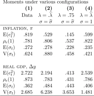
The MDE procedure also allows to test for over-identifying restrictions, i.e. the null hypothe-sis that the set of K moments µ can accurately be described with the P parameters to be es-timated i.e. the elements of λ and Σv. The test statistic is given by the objective function [_bµ−µ(λ,Σv)]0Ωb−1[_bµ−µ(λ,Σ_v)]. Here, rather than relying on the asymptotic Chi-square distribu-tion, we will use Monte Carlo simulations of the model to approximate the exact small distribution of the test statistics.

27