48th AIAA Aerospace Sciences Meeting and Exhibit AIAA 2010-1576 4 - 7 January 2010, Orlando, Florida
Experimental Space Shuttle Orbiter Studies to Acquire Data
for Code and Flight Heating Model Validation
T.P. Wadhams*, M.S. Holden†, M.G. MacLean‡
,
CUBRC, Buffalo, New York
Charles Campbell§,
NASA Johnson Space Center, Houston, Texas
Abstract
In an experimental study to obtain detailed heating data over the Space Shuttle Orbiter, CUBRC has completed an extensive matrix of experiments using three distinct models and two unique hypervelocity wind tunnel facilities. This detailed data will be employed to assess heating augmentation due to boundary layer transition on the Orbiter wing leading edge and wind side acreage with comparisons to computational methods and flight data obtained during the Orbiter Entry Boundary Layer Flight Experiment 1 and HYTHIRM2 during STS-119 reentry. These comparisons will facilitate critical updates to be made to the engineering tools employed to make assessments about natural and tripped boundary layer transition during Orbiter reentry. To achieve the goals of this study data was obtained over a range of Mach numbers from 10 to 18, with flight scaled Reynolds numbers and model attitudes representing key points on the Orbiter reentry trajectory. The first of these studies were performed as an integral part of Return to Flight activities following the accident that occurred during the reentry of the Space Shuttle Columbia (STS-107) in February of 20033. This accident was caused by debris, which originated from the foam covering the external tank bipod fitting ramps, striking and damaging critical wing leading edge heating tiles that reside in the Orbiter bow shock/wing interaction region. During investigation of the accident aeroheating team members discovered that only a limited amount of experimental wing leading edge data existed in this critical peak heating area and a need arose to acquire a detailed dataset of heating in this region. This new dataset was acquired in three phases consisting of a risk mitigation phase employing a 1.8% scale Orbiter model with special temperature sensitive paint covering the wing leading edge, a 0.9% scale Orbiter model with high resolution thin-film instrumentation in the span direction, and the primary 1.8% scale Orbiter model with detailed thin-film resolution in both the span and chord direction in the area of peak heating. Additional objectives of this first study included: obtaining natural or tripped turbulent wing leading edge heating levels, assessing the effectiveness of protuberances and cavities placed at specified locations on the orbiter over a range of Mach numbers and Reynolds numbers to evaluate and compare to existing engineering and computational tools, obtaining cavity floor heating to aid in the verification of cavity heating correlations, acquiring control surface deflection heating data on both the main body flap and elevons, and obtain high speed schlieren videos of the interaction of the orbiter nose bow shock with the wing leading edge. To support these objectives, the stainless steel 1.8% scale orbiter model in addition to the sensors on the wing leading edge was instrumented down the windward centerline, over the wing acreage on the port side, and painted with temperature sensitive paint on the starboard side wing acreage. In all, the stainless steel 1.8% scale Orbiter model was instrumented with over three-hundred highly sensitive thin-film heating sensors, two-hundred of which were located in the wing leading edge shock interaction region. Further experimental studies will also be performed following the successful acquisition of flight data during the Orbiter Entry Boundary Layer Flight Experiment and HYTHIRM on STS-119 at specific data points simulating flight conditions and geometries. Additional instrumentation and a protuberance matching the layout present during the STS-119 boundary layer transition flight experiment were added with testing performed at Mach
* Research Scientist, AAEC, CUBRC, 4455 Genesee Street, Buffalo, NY, Senior Member. † Vice President, Hypersonics, AAEC, CUBRC, 4455 Genesee Street, Buffalo, NY, Fellow. ‡ Senior Research Scientist, AAEC, CUBRC, 4455 Genesee Street, Buffalo, NY, Senior Member.
§ Aerospace Engineer, NASA Johnson Space Center, 2101 NASA Parkway, Houston, TX, Senior Member.
48th AIAA Aerospace Sciences Meeting and Exhibit AIAA 2010-1576 4 - 7 January 2010, Orlando, Florida
number and Reynolds number conditions simulating conditions experienced in flight. In addition to the experimental studies, CUBRC also performed a large amount of CFD analysis to confirm and validate not only the tunnel freestream conditions, but also 3D flows over the orbiter acreage, wing leading edge, and control surfaces to assess data quality, shock interaction locations, and control surface separation regions. This analysis is a standard part of any experimental program at CUBRC, and this information was of key importance for post-test data quality analysis and understanding particular phenomena seen in the data. All work during this effort was sponsored and paid for by the NASA Space Shuttle Program Office at the Johnson Space Center in Houston, Texas.
I. Introduction and Program Overview
The primary purpose of this test program (designated M11-13) was to perform tests at Mach Numbers of 10, 14, 16, and 18, with matched flight Reynolds Numbers at model scale to obtain detailed laminar and turbulent heat transfer measurements on the wing leading edge of the Space Shuttle Orbiter in the peak heating shock interaction region. These measurements would be used for CFD code validation and to update the engineering tools that are used to predict pre-flight reentry heat loads to the Orbiter. Other objectives included obtaining centerline and attachment line transition data at high Mach numbers; and acquiring model attitude and control surface deflection data over a range of Mach numbers and Reynolds numbers
Acquiring this data became a priority for NASA following the Colombia tragedy, and in light of the limited amount of experimental wing leading edge heating data that was available to evaluate damage that might occur during ascent on Shuttle flight. Prior to Colombia there were only a limited number of experimental wind tunnel Orbiter heating tests that had been conducted to collect wing leading edge data. Of this group, only one test was considered accurate enough with a high enough resolution of heat transfer sensors to be considered the as reference for wing leading edge heating. That model, designated O11-66, contained only one detailed chord-wise heating strip in the peak heating shock interaction region and fixed the span-wise peak heating to this location. The limited amount of data also posed a risk to the program described here in this report; even with a large amount of instrumentation it may still be possible to miss the wing leading edge peak heating location. As an added difficulty, the three-dimensional geometry and shock wave boundary layer interaction made prediction of the peak heating in these types of flowfields by the most accomplished computationalists using today’s state-of-the-art codes difficult at best.
The Orbiter Entry Aeroheating technical leadership, endorsed by the Space Shuttle Orbiter Project, chose CUBRC’s LENS I Hypervelocity Shock Tunnel Facility to meet these goals because of the facility’s ability to match the required reentry trajectory test conditions and because of CUBRC’s ability to instrument the Orbiter wing leading edge with a large amount of highly accurate thin-film sensors. The LENS I facility was also ideal due to the delicate nature of the thin-film sensors and the necessity to obtain data over the series of Mach Numbers, Reynolds Numbers and model attitudes with little loss to the valuable sensors.
A separate but equally important part of the test is CUBRC’s CFD analysis that has been done to validate and verify every aspect of the test from confirming tunnel calibration results and aiding in the design of tunnel hardware to the pretest predictions of the model flow fields and heating level estimates. CFD calculations before any testing is done and throughout the entire testing process have become an integral part of any test program completed at CUBRC. This work will be discussed in more detail later in this document.
Additional studies will be completed in the near future with the M11- 13 model to compare to experimental data obtained during reentry of STS-119. The model will be modified with additional instrumentation to match those present during the reentry flight along with replication of a boundary layer trip placed on the model to induce boundary layer transition on the windside wing acreage of the Orbiter. This experimental data and the corresponding computational results will go a long way to further the understanding of the differences of boundary layer transition in experimental facilities, computational codes, and flight.
II. Facilities and Instrumentation A. The LENS Facility
The aerothermal tests in this program were performed in the LENS I and 48 inch Tunnel hypervelocity reflected shock
tunnels. A schematic diagram of the LENS I HST is shown 1 ^sr\ alongside the LENS II facility in Figure 1. The two facilities -. y
share a common control system, compressor system, data recording system and data analysis system. LENS I has the capability to fully duplicate flight conditions at Mach numbers
ranging from 6 to 15, while LENS II has similar capabilities 3omo __° ^ ^^
from Mach 3 to 9. A photograph showing the three LENS
facilities at the Aerothermal Aero-Optics Evaluation Center Figure 1. Schematic Drawing of the LENS I (AAEC) can be seen in Figure 2. and LENS II Hypersonic Shock Tunnel
The major components of the LENS I facility include a Facilities and LENS X Expansion Tunnel 25.5-foot long by 11-inch diameter electrically heated driver
tube, a double diaphragm assembly, a 60-foot by 8-inch diameter driven tube, a fast acting centerbody valve assembly, multiple nozzles to achieve desired test conditions from Mach 7 to 18, and a test section capable of accommodating models up to 3 feet in diameter and 12 feet long. The LENS II facility is similar in construction, incorporating 24-inch driver and driven tubes that are 60- and 100-feet in length respectively and is currently
r ^{ a capable of running between Mach 3 and 9.
IF ( ^' !j'^ The high-pressure driver section of LENS I has the
ti `'" f, f - uu^^
capacity to operate at 30,000 lbf/in2 using heated driver gases of hydrogen, helium, nitrogen or any combination of the three. The driver gases can be heated up to 750°F and the amount of each gas varied to achieve tailored interface operations for maximum test times. The driven tubes of either facility can use air, nitrogen,
- carbon dioxide, helium, hydrogen or any other gases or
combinations of gases for model testing.
A schematic diagram illustrating the basic operation of the shock tunnel is shown in Figure 3. Both LENS I and LENS II Figure 2. Photograph of the LENS I and tunnels operate with tailored interface conditions to maximize LENS II Facilities at the Aerothermal Aero- test condition uniformity and run time. Tailored conditions are Optics Evaluation Center achieved by carefully controlling the pressures and gas mixtures used in the driver and driven tubes of the tunnel to achieve a condition where the contact surface between driver and driven gases is transparent to the reflected shock. Flow is initiated through the tunnel by rapidly pressurizing the center
^rNer Ele,b pll Healer 1ti h 1h,,k Ebainles Mylar._ Test MOtlel
section of the double diaphragm unit causing the diaphragms f, — -p-g. I
to rupture. The sudden release of the driver gas generates a
1;
—
Csnte B tly strong shock which travels down the driven tube, is reflected ^as ^ ° . TeVam Tank^^C°mpre
r Carry 8h,k Wad eletl Ion
from the end wall, and travels back up the driven tube, L__ 'T11 Stb d bv
creating a stagnant, high-pressure, high-temperature reservoir ^^
of test gas. When the reflected shock strikes the interface in k aVe
its return path, the condition in the driver and driven tubes ^_ +,:d ^;"^^f`o^w'IadPrManel
are controlled such that the contact surface is brought to rest.
-s,ead F
The reservoir of hot stationary test gas between the end wall [ ;{ ---III ^^ T ro°gnr nnal
and the contact surface is exhausted through the throat
III' f ^^ Center Botly Closet
section of the nozzle into the test section in a manner similar i - ---- ^L^ aaA^°wE°da
to any blowdown tunnel. The flow through the nozzle is Figure 3. Basic Operation of the LENS terminated when a fast-acting valve closes the throat section. Facilities
The LENS II facility has three contoured nozzles
that allow operation from Mach 3.5 to 9 with test times between 100 and 20 msec at velocities from 3,000 to 9,000 ft/sec respectively. A velocity/altitude map for the LENS facilities is shown in Figure 4. By operating the LENS tunnel under cold conditions (just above the liquefaction temperature of the airflow in the test section), large
Figure 5. Mach Number/Reynolds Number Envelope Figure 4. LENS Facility Altitude Velocity Map
Reynolds numbers and test times can be obtained in the LENS I facility for studies where only Mach number, Reynolds number simulation is required. A Reynolds number and Mach number performance plot for the LENS facility is shown in Figure 5. Additional information concerning the LENS facilities as well as the AAEC’s capabilities can be found in the references [AAEC Research Staff 2004].
B. Heat Transfer Instrumentation
For these studies we employed thin-film heat transfer instrumentation similar to those designed at Cornell Aeronautical Laboratory (CAL) in the late 1950s and refined over the past 50 years. The platinum thin-film heat transfer instrumentation employed in these studies have proven to be the most accurate measurement technique in supersonic and hypersonic test facilities, and the small size of the sensing element coupled with the insulating substrate make them ideal for a high resolution measurements CUBRC has calculated the
accuracy of the heat transfer measurement to be ±5%. Figure 6b. 0.125” Thin-film
Figure 7. MH-13 Port Side Wing Leading Edge Thin-film Pyrex Inserts
Figure 8. Macor Insert in Starboard Wing Leading Edge
The thin-film heat Heat Transfer Instrument transfer gauge is a resistance
thermometer that measures the local surface temperature of the model. The theory of heat conduction is used to relate the surface temperature history to the rate of heat transfer. Since the
Figure 6b. 0.050” Thin-film platinum resistance element has
Heat Transfer Instrument negligible heat capacity, and
hence negligible effect on the Pyrex surface temperature, the gauge can be characterized as being homogeneous and isotropic with properties corresponding to those of the Pyrex (Videl 1956 and Cook and Felderman 1966). Furthermore, because of the short duration of shock tunnel tests, the Pyrex can be treated as a semi-infinite body. The same is true for Macor, which was also employed in this test to allow for the instrumentation of the starboard wing leading edge. While this application was ideal for Macor due to the ease at which it can be shaped, Pyrex was used everywhere else due to its superior durability. Examples of the types of thin-film instrumentation employed in this test can be seen in Figures 6-8. Unique to this test are the leading edge Pyrex inserts and the Macor leading edge insert shown in figures 7 and 8 respectively. The Pyrex inserts were cut and shaped as a single piece of glass to match each wing span location and then had the platinum
sensor painted at the desired location in the chord wise direction. The sensors were tightly packed in the peak heating region and spread out on both the windward and leeward sides. In all more that 200 platinum thin-film sensors were present in these inserts. The Macor leading edge on the starboard side of the model contained 30 thin-film sensors that represented twice the density in the peak heating region in the span-wise direction compared to the Pyrex based inserts on the port side of the model.
C. Pressure Instrumentation
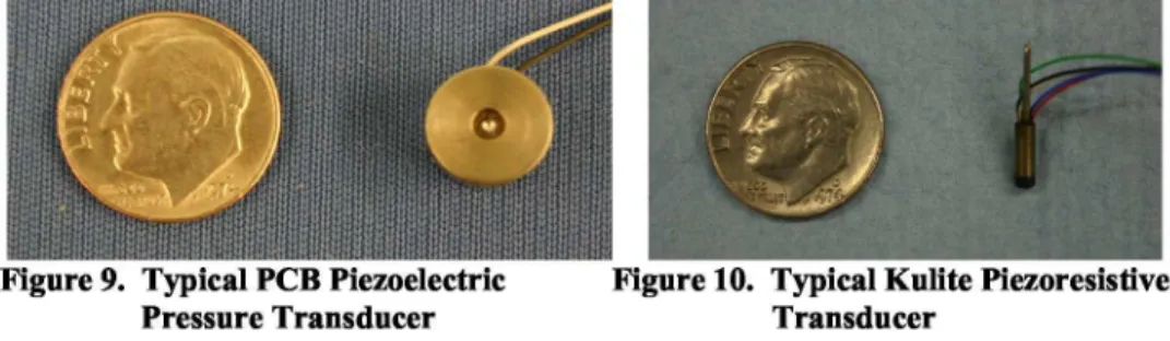
For these studies, we primarily employed piezoelectric pressure gauge instrumentation that, like the platinum thin-film sensor, was originally designed at Cornell Aeronautical Laboratory. These gauges employ a diaphragm design and read the model pressure versus a pretest baseline pressure (differential pressure). In the data reduction process this baseline, or pre-run pressure, is subtracted off the final measurement to yield an absolute measurement. Additionally, these transducers are mounted close to the surface of the test article so that orifice effects and fill times are negligible. The piezoelectric pressure transducers, manufactured by PCB, are capable of accurately measuring pressures within ±3%. Figure 7 shows a typical PCB piezoelectric pressure transducer.
Where size constraints do not allow for PCB style instrumentation CUBRC employs both Endevco and Kulite piezoresistive type transducers. These transducers have a very small sensing footprint and can be installed in difficult geometry locations. These sensors also typically have a higher frequency response (~100 kHz) than the standard piezoelectric sensors we employ. The piezoresistive strain gauge-type transducer also has an accuracy of ±3%. Figure 8 shows a typical Kulite style transducer.
Pressure gauges employed by CUBRC are calibrated installed in the test article whenever possible. Calibration is carried out by subjecting each gauge to a traceable, steady pressure pulse lasting tens of milliseconds to duplicate what the gauge will experience during testing. This will occur over the range of expected pressures that the gauges will experience during testing.
Figure 9. Typical PCB Piezoelectric Figure 10. Typical Kulite Piezoresistive
Pressure Transducer Transducer
III. Model Design and Construction A. 1.8% Scale Risk Mitigation Phase Orbiter Models
CUBRC designed, constructed and instrumented the 1.8% scale steel and aluminum MH-13 model using configuration and outer mold line data supplied by the NASA team. CUBRC contracted EverFab, a local high-fidelity fabrication shop, to build this model due to the high OML tolerances that could be maintained and inspected. The first model constructed was made from RenBaord, an inexpensive epoxy-based material used for quick prototyping. Fabrication of the RenBoard model was done to ensure the files provided by NASA were of machine fabrication quality, and that EverFab would be able to construct the Orbiter to NASA’s tolerances and specifications. This verification and acceptance of the Renboard model primarily meant that the file CUBRC was designing from itself was considered to be of ”machine quality”, meaning that the file did not have gaps or unconnected surfaces that the machining software had to interpret in order to construct the model. The primary concerns for model construction and data analysis were surface smoothness, dimensional and geometric variances, as well as being able to ascertain model coordinates via the temperature sensitive paint video imaging system. In addition, a critical design aspect was to provide a means of rigidly placing fiducial points along the model at known locations by taking measurements of the placed points with respect to the model geometry. After the drawing file was checked for machine fabrication quality, design of the peripheral hardware needed for testing the model in LENS I was completed. The sting assembly used in this series of tests is shown in Figure 11. The sting assembly was fabricated such that multiple angles of attack could be achieved with minimal time to adjust the model and assembly to the desired pitch angle. In addition, a small yaw-plate was constructed to be inserted between the model
and sting assembly for test conditions that required a yaw angle. Due to the uncertainties of the different model attitudes to be studied, the yaw-plate and sting assembly were designed to be readily modified with minimum time for machining and/or assembly. In order to accurately measure the pitch and yaw of the model’s orientation, a pitch/yaw measuring plate was fabricated in which the plate, bushings and mounted holes were machined with respect to the model centerlines. The
~ [uig?Dd'a^mt: variance due to machining of the measured pitch/yaw angles was calculated
to be ± 5 minutes. A drawing of the pitch/yaw measuring plate is shown in Figure 12. Finally, prior to testing, all of the model components were
-^ * stressed to four times the highest load the model would be subject to in the
test matrix. This included the model, yaw plates, and sting hardware. 4 * The primary challenge of the detailed design of the model was in
making it versatile enough to incorporate the large amount of instrumentation, be able to accept the various cavity and trip blocks and rings, have the required movable control surfaces, and still pass the loads Figure 11. MH-13 Sting Assembly requirements of testing in the LENS I facility. The steel fuselage component remained one solid piece that attached to the sting assembly and carried the loads of the attached wing and centerline components. The forward (X/L=0.3) trip and cavity block as well as the aft (X/L=0.5) trip and cavity ring can be seen as well as the port thin-film inserts. These inserts were each made from a single piece of Pyrex that was individually cut and shaped to exactly match the wing outer mold
line at a particular span station. Each Pyrex insert had fourteen platinum
thin-film instruments painted on them and were set with epoxy into the ,.
appropriate wing leading edge slot (Figure 13). Allowances were also -; ter,_ made along the centerline, wing acreage, and control surfaces for an ^5a additional 100 sensors to measure centerline and attachment line heating r
-changes resulting from model attitude -changes and boundary layer T transition. This capability was augmented with adding a uniform depth N cavity machined into the starboard wing acreage to accept temperature ; ,_,__,.^ sensitive paint insulator and sensing coats while still matching the
required outer mold line geometry. The temperature sensitive paint will Figure 12. Pitch/Yaw Plate for Use look at the global effects of transition while the more accurate thin-films with CUBRC Inclinometer
will look at the temporal effects.
Between the first and second entries of the model modifications were made to accept a trip ring at X/L=0.3, instead of just a centerline block, and additional instrumentation was added to fulfill newly expanded testing goals. This included the addition of a Macor wing leading edge insert on the starboard side of the model (Figure 8) that featured double the number of span-wise thin-film sensors in the wing leading edge peak heation region when compared to the port side. The new instruments
,r- - _ would further map out the peak heating locations and
' 1 -- — - serve as a check of the data from the port side of the
-',` ! , `- • _ ^._ " - - model. Additional trips and cavities were also
- '• _ j manufactured to assist in the acquisition of a larger
dataset of high Mach number boundary layer transition data on the centerline and wing acreage.
_ rid r A third entry is currently planned for the early
. •, 2010 with the addition of 20 thin-film sensors matching locations on the STS-119 Flight Boundary Layer Transition Experiment. Additional trip elements will Figure 13. MH-13 Wing Leading Edge Thin-film also be constructed to simulate the boundary layer trip
Pyrex Inserts present on the flight.
IV. Experimental and Computational Facility Flow Calibrations
Each unique test condition to be run during the experimental program is first calibrated with test runs in the facility and is also predicted computationally. These computational predictions allow for having to make fewer tunnel calibration runs at each condition and more importantly, it adds greatly to the understanding of what is
occurring in the freestream at every condition. This
becomes important later when full 3D model ^ Plrotn.._^eres=,Nn,ferm,ry
computations are preformed. Basic instrumentation Mach Numder
associated with the experimental calibration of the LENS
facilities include: pressure sensors to monitor the initial "—'^`^— } ° c^ driver and driven gas pressures and temperatures,
thin-film resistance gauges installed at fixed locations on the driven tube to monitor incident shock wave speed as it propagates down the tube, pressure sensors in the endwall
.
region to measure the reflected shock reservoir pressure, Ca id t en Rak a and s ag P ess°re
Arse my vaadate Start Pressure
a pressure sensor in the initially evacuated test section, Nozzle Heat Transfer __ r StagnationHeat Transter
-Confi rm and Select -Ch ck Total Temperature
and a survey rake installed in the test section to measure theComputational .__ „. Models used to
pitot pressure, static pressure and stagnation point heat valldat,adrTeat
Conditions and Pmvidd
transfer in the freestream. From these measurements and Additional Information
°n Flow Cha ,a r LENS I Call cratlon Rake Installation Drawing
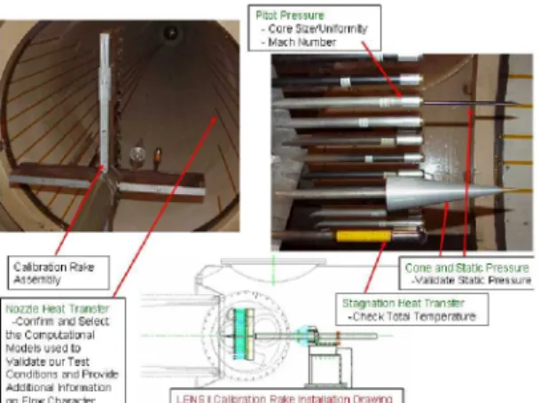
rake assembly, a comprehensive data set for each test Figure 14. Photograph of Pitot Rake Assembly condition was taken to calculate freestream conditions, Mounted Inside Test Section of the LENS II core size, and flow uniformity of the freestream flow. A Hypersonic Shock Tunnel
typical survey rake assembly is shown in Figure 14 together with the flowfield survey probes at the exit plane of the nozzle at the same station the Shuttle Orbiter
model placed during the program. '
High-frequency pressure instrumentation is
typically used in the pitot probes; however, in regions , where flows generate high thermal loads, we must
employ thermal protection systems in order to lower the frequency response. Total temperature measurements are made in the lower enthalpy flows with shielded
thermocouple probes, while total heat transfer o 0 0 o
measurements are made with miniature thin-film or '•^ ° °"'
coaxial instrumentation placed in the stagnation region of
Figure 15. Comparison between Experimental a hemispherical nosetip.
and Computational Nozzle Pitot Pressure Profile The first step in determining the test conditions
in LENS facility is to determine the conditions observed in the reservoir. This is accomplished via a combination of measurement and theory. The initial and final (reservoir) pressures are measured by a group of redundant pressure gauges in the endwall of the driven tube. The shock speed is also measured by a series of fast-response gauges down the length of the driven tube which react as the incident shock moves through the test gas. Employing this information, the unique reservoir conditions may be computed from generalized equilibrium conditions and wave propagation theory after both the incident and the reflected shocks have passed through the test gas. The computation of the reservoir assumes full thermodynamic and chemical equilibrium at all points. This is a safe assumption, as the pressures and temperatures after the shocks are very large, thus making relaxation times exceptionally short. Relevant translational, rotational, and vibrational modes are considered in the energy of the molecules.
The results were then compared with the pre-calibration computational results. Figure 15 shows an example of the comparison of the Navier-Stokes and the measured pitot profile measurements for Mach numbers of 10, 14, and 16, demonstrating the level of agreement obtained between CFD and experiment in the LENS programs. Pitot pressure is used as a measure of freestream accuracy for two primary reasons: (1) it is a directly measurable quantity, and (2) it is sensitive to the momentum in the flowfield; hence, it is a good choice to judge the accuracy of the freestream specification. The computations were preformed with the DPLR Navier-Stokes solver [Wright, et al. 1998] that had been modified specifically to solve the nozzle flow problem in the LENS facility. As stated earlier in this section, the excellent results obtained from these computations allow for fewer facility calibration runs and give CUBRC and the customer a greater understanding of the freestream conditions in the facility. This process of performing both experimental and computational has become the standard procedure CUBRC employs to prepare for any experimental program in the LENS facility.
V. The Experimental Studies A. Pre-Test and MH-12 Risk Mitigation Phase
The experimental program began with an extensive literature search for data to aid in the placement of the wing leading edge instruments in order to capture the peak heating locations over a range of Mach numbers, Reynolds numbers, and model attitudes. The peak heating is fundamentally due to the shock boundary layer interaction of the bow shock from the nose of the Orbiter impinging on the wing leading edge. A typical Schlieren image of this shock wave can be seen in Figure 16. Available literature included data from the OH-66 Shuttle
Orbiter wing leading edge test performed at Calspan (the predecessor of CUBRC) in 1978 [Wittliff, et al. 1978]. While several aerothermal tests were conducted to obtain wing leading edge heating data, the OH-66 test remained the only detailed wing leading edge aerothermal test to be conducted on the Shuttle Orbiter until the current test described in this report. The data from OH-66 became the basis, along with key flight data calibrations, for the engineering tool that is still used today to predict mission heating loads. Several photos of this test model can be seen in Figure 17. The model was a 2.5% scale replica of the existing outer mold lines that Figure 16. Typical Schlieren Image of Shock contained four densely populated thin-film sensor strips at 40, Interaction Due to Bow Shock from Orbiter 55, 80, and 90 percent of semi-span. Of these four insert
locations only the 55 percent position was placed in the shock interaction peak heating region. Also questions existed as to what the outer mold lines of the model actually looked like when compared to current Orbiter CAD files because the model has been destroyed since the end of the test program. In the end it was determined that the OH-66 data, with additions from current computational predictions ,was not enough to confidently place the large number of sensors necessary to map out the interaction peak heating region within the required time or resources available for the test.
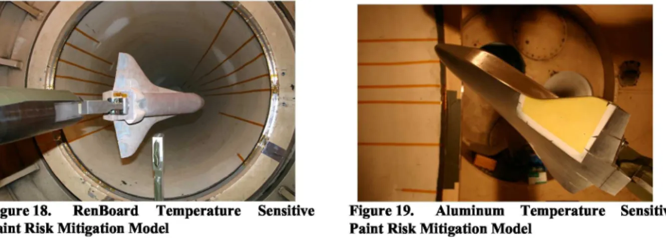
To mitigate the risk to the program, CUBRC suggested performing a preliminary set of tests on the model Figure 17. OH-66 Aerothermal Model geometry with temperature sensitive paint to map out the peak heating region. This risk mitigation phase, designated MH-12, was broken up into three distinct parts. The first part consisted of a limited number of facility calibrations to check flow uniformity, core size, and test time to allow CUBRC to size and locate the model and to start the temperature sensitive paint checkout process. These calibrations confirmed that the proposed 1.8% scale Orbiter model would be well inside the uniform core flow of LENS I over the vast majority of required test conditions. The first Orbiter model to be tested was a plastic RenBoard model that served as the machining test model for Everfab, the
Figure 18. RenBoard Temperature Sensitive Paint Risk Mitigation Model
Figure 19. Aluminum Temperature Sensitive Paint Risk Mitigation Model
manufacturer of the models to be used in this series. This RenBoard model, shown in Figure 21, was the machine drawing qualification model that was manufactured first to ensure proper manufacturing of the actual metal model to follow. The twelve runs completed in this series were made solely to confirm the experimental setup and techniques necessary to film the wing leading peak heating locations with temperature sensitive paint durring the time that the follow-on aluminum model was being manufactured by Everfab. Fourteen test runs were completed with the aluminum model, shown in Figure 22, employing Figure 20. Typical Wing Leading Edge temperature sensitive paint to map out the locations of Temperature Sensitive Paint Results Showing the peak heating while sweeping through Mach number,
Location of Peak Heating Reynolds number, angle of attack and yaw. This
temperature sensitive paint data was backed up on the other side of the model with thin-film instrumentation painted onto a Macor insert which can be partially seen at the bottom of the model in Figure 22.. An example of the temperature sensitive paint data collected can be seen in Figure 20 [Smolinski. The acquired temperature sensitive paint and high speed schlieren information were directly used along with the limited OH-66 and computational results to specify where the wing leading edge instrumentation should be placed. Detailed information concerning the temperature sensitive paint technique can be found in the references. [Hubner, et al. 2002].
C. The Main MH-13 Shuttle Orbiter Test Program
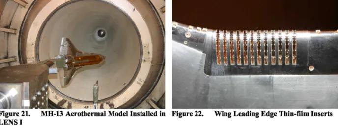
The main part of this program followed the risk mitigation phase after the design, manufacture, instrumentation, and assembly of the new steel and aluminum MH-13 model was completed. This new model was initially instrumented with 288 sensors, over 200 of which were on the wing leading edge, and the rest (over 80 in number) were located on the body centerline, wing acreage, and control surfaces. These acreage sensors were added to meet secondary objectives of centerline and attachment line boundary layer transition, centerline and acreage angle of attack and yaw data, and control surface deflection data. The starboard side of the model was also setup to utilize temperature sensitive paint to get global images of the transition process. Photographs of this model, instrumentation, and temperature sensitive paint regions can be seen in Figures 21-23.
Like the risk mitigation phase of the program, the main part was also broken to several distinct phases, the first of which consisted of a new series of calibration runs representing Mach number and Reynolds number sweeps along the nominal flight reentry trajectory including prescribed trajectory excursions limits. Mach Numbers of 10, 14, 16, and 18 were surveyed with sample calibration data shown in Section IV. After completion of the calibration tests the steel and aluminum MH-13 model was installed in LENS I and tested to meet the primary objective of mapping wing leading edge laminar and turbulent heating over a reentry range of Mach numbers, Reynolds numbers, and model attitudes. Determination of the turbulent heating increment above the laminar value on the wing leading edge was of key importance to bound the :
Figure 21. MH-13 Aerothermal Model Installed in Figure 22. Wing Leading Edge Thin-film Inserts LENS I
interaction region. Beyond wing leading edge heating data, secondary goals included centerline and attachment line boundary layer transition studies and acquiring acreage and control surface data at various model and control surface attitudes. An example of smooth wall, no trips or cavities, boundary layer ( transition is shown in Figure 24. Here the model was tested at the same angle of attack over a range of Reynolds numbers to observe the location of boundary . ° layer transition and the heating augmentation due to the r turbulent flow. The date is from the sensors along the
centerlone of the Orbiter from the nose to the end of the body flap as shown in Figure 23. The body flap in this Figure 23. MH-13 Model Overview Showing case for all runs shown but one has been deflected 13 Yellow Temperature Sensitive Paint Regions degrees. This deflection results in a separated region in the laminar forebody cases (Runs 1 and 2) near the 26
0:8
inch station. The flow then reattaches near the 28 inch ,ROnf1 (Mach(lQ R 4 ES Ann=40^Y O,,BF 13 AL '10)
i07 ' - ,REn2 (Mach `10', ^, Re 82E5 ^;oA=40 1Yan Q,,BF 13 AL 'ia) _-- station and then the boundary layer begins to transition =O;;BF 45 A^-' to turbulence. This is evident from the character of the
RIn'l 1' (Mach (10„ Re 22E6 AoA 40^Yaw-O„BF 13 PL-10 V.6 4,R^n 19 ((Mach rO,,R 32E6 lio:4 40 tY 71
2,REn 1321(Mach X10 Re 11(4E6,'AoA) A^°^ `Yaw=O BF_'13°,'AL 3°j time history trances in this area and higher heating rates X0'5 - - CUBR"Laminar'solution MacLean —
than the corresponding laminar CFD solution which will
4 -
- be discussed more in a later section. A further increase
0.3 in Reynolds number (Run 11) moves the boundary layer
r• ^• r. a ' transition point ahead of the separated region location at
0°2
, lower Reynolds numbers and allows the flow to stay
attached longer and significantly shortens the separated I I
0 region. The data from this condition appears to be fully
'0 (5
11
r5 '20 25 30 turbulent on the body flap due to the decrease in heating
Distance from Orbiter Reference`(inches)
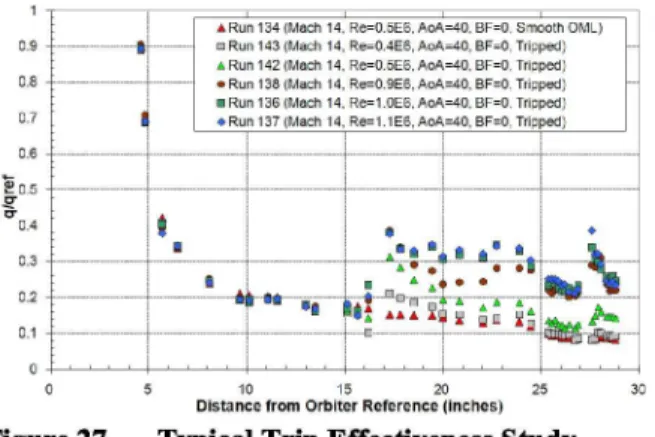
Figure 24. Orbiter Centerline Transition Example rate after the reattachment point. There are two more Reynolds number increases presented (Run 19 and 132) which both successively move the transition point further forward toward the nose of the model. The NASA team also desired to obtain data on the model with protuberance (trip) and cavity induced boundary layer transition to test engineering tool developed at NASA Langley Research Center to predict the effectiveness of these cavities and protuberances in flight. To obtain this data CUBRC manufactured, and in some cases instrumented, a series of protuberances and cavities prescribed by LaRC to achieve incipient transition. The protuberances included both diamond trips and wedge like fences that represented protruding gap fillers in flight. Cavities varies from long and shallow, to short and deep, to sloping bottoms reminiscent of real cavities documented during flight. An example of the protuberances and cavities used in this phase are shown in Figures 25 and 26. The incipient transition point
Figure 25. Photograph of a Typical Protuberance Figure 26. Photograph of an Instrumented Cavity (trip) Employed during MH-13 Testing Employed during MH-13 Testing
15 I' 17 19
t
1a 201 L22 L2 4 Di stance;fromfbr[gin ((incheSl', 44 y Flapo
40 44 - 36- y 2533 ze ze L 40time-history traces and looking for the first signs of
'Run 134 (Mach 14 Re O.5E6 AoA 40 BF- Smooth 13ML)
;0.9 ----} o R n 143 (Mach 14 R V.: E6 A A 40 BF T .,ped; - transition. A typical centerline data profile over a range
i Ruri 142 (Mach 14 Re-05E6 AcA 40 BF '0 Triaped; TT
!0.8 •Run'138 (Mach 14 R =0.9E6 A 40 BF 0 T 'cped; - of Reynolds numbers can be seen Figure 27. ere withm H
. Run,36 (Mach ,4 Re'V1E6 PAoA 40 BF=0 Tr(oped)
the data correlated to collapse the upstream laminar data
'0.7 it '♦RUn`167i(fdach 14 Re=^1 .1 E6 PoA 40 BF=0 Tricped;
0.6 -- --- -- - we see where the data begins to depart and transition from
__ _ _ ___ _ ____- laminar to turbulent heating. Additionally one can
observe the time histories of the thin-film heat transfer
- Ak < a , sensors and see evidence of bursts of turbulence that break
o. __ + • - -J out. These turbulent bursts travel downstream and
•'•'° 4 QL coalesce with other turbulent bursts that break out and
ti
0 eventually form the turbulent boundary layer. An
0 15 X10 5 20 X25 3o example of this process is presented in Figure 28 which
bistance'from "Orbiter Reference(inches)
Figure 27. Typical Trip Effectiveness Study details with number callouts sections of the model that are laminar, transitional (signs of turbulent bursts), and fully turbulent. The bursts are observed in the time histories as large spikes in the heating and with a sufficient number of thin-film sensors can be tracked as the travel downstream. Following the time sequence of the thin-films the increase in the number of turbulent bursts and how they coalesce can be observed.
Laminar Turbulent C Additional
Fj 1 7 1
First Indication of 19 I 25 33 Turbulent Bursts
Transition Region Peaks
Turbulent Bursts
36 'Turbulent BuCoalesce
9 13
2 Ll'4
Figure 27. Boundary Layer Transition Behavior Observed During MH-13 Studies
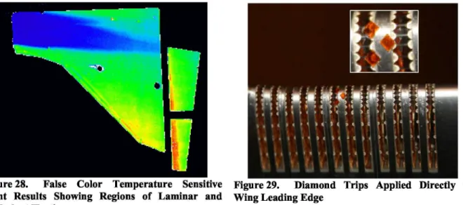
Temperature sensitive paint images were also taken during this phase to access the global effects of transition on the wing acreage. The temperature paint section of the model can be seen in yellow in Figure 23. These images were taken to observe the extent and locations of the turbulent wedges as they occur on both smooth body runs and tripped runs. An example of a typical temperature sensitive paint image can be seen in Figure 28. In the figure laminar regions are colored blue with turbulent data showing up in green to yellow on the wing acreage. The wedge of turbulent flow from the centerline of the model, toward the top of the figure, and from the attachment line, toward the bottom of the figure, can be seen.
Between the first and second entry of this phase of the program the model was reconfigured for additional wing leading edge sensors and new protuberances and cavities were built. The model was modified with a new wing leading edge insert (Figure 8) made of Macor and instrumented with 20 thin-film sensors placed directly on the surface and new locations for trips and cavities to be installed. Researchers wanted this additional wing leading
Figure 28. False Color Temperature Sensitive Figure 29. Diamond Trips Applied Directly to Paint Results Showing Regions of Laminar and Wing Leading Edge
Turbulent Heating
edge instrumentation set to obtain wing leading edge heating data on the starboard side of the model, mirroring the original thin-film wing leading edge inserts on the port side, to check the data from the first entry and to achieve double the resolution in the peak heating shock interaction region in the span-wise direction. The second entry began with several new facility calibration runs to cover new boundary transition conditions and to confirm existing conditions. During this second entry the primary objective was the confirmation of turbulent heating increments above the laminar values in the peak interaction region. The data was acquired with smooth body, attachment line trips on the body, and a set of trips that was even applied directly to the wing leading edge. Examples of these wing leading edge trips can be seen in Figure 29. The turbulent wing leading edge data was checked against smooth and tripped data from the firstentry, the new starboard side mirror gauges, and versus smooth body and tripped data with trips placed at several different locations on the body to confirm the turbulent heating increment using the Stanton number correlation method mentioned in the pervious phase. A secondary objective that encompassed a majority of test runs in this phase focused on acquiring boundary layer transition data with a new set of protuberances and cavities that in some cases resembled geometries that could be present in flight. As before, the incipient transition point was determined with a Reynolds number survey. Temperature sensitive paint data was again taken to observe the global transition behavior along the centerline and attachment line wing acreage locations as shown in Figure 31. D. Future Studies with the MH-13 Model to Match Flight Results
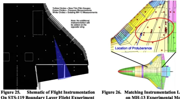
In the spring of 2010 a new entry has been planned with a further modified MH-13 model. This new entry will acquire experimental data to compare to data taken during the reentry flight of STS-119 (Campbell Referecne XXXX). This Orbiter mission included a number of TPS tiles on the wing acreage that were replaced with tiles containing thermo-couple sensors to measure the surface heating as the Orbiter passed through the atmosphere. These sensors were placed on the wing to observe the state of the boundary layer behind a protuberance that was likewise placed in the center of a new surface tile. The layout of these sensors and the location of the protuberance during flight can be seen in Figure 30 with the proposed layout on the MH-13 model shown in Figure 31. The CUBRC experiments will duplicate these locations and employ a boundary layer scaled protuberance simulating the flight article. The model will also include a scale protuberance on the temperature sensitive paint side of the model to observe the extent of the turbulent wedge produced by the protuberance. This data could additionally be compared to infrared measurements of the windside of the Orbiter as part of the HYTHIRM program. Freestream conditions for these studies will be selected to match Mach number and the model scaled Reynolds number of key points of interest for boundary layer transition. This experiment will represent another important opportunity to assess differences in the character of boundary layer transition between prediction, ground testing, and flight results to build toward improved methodologies for the prediction of boundary layer transition on future high speed flight vehicles. CUBRC is also working toward having this key comparison between flight, ground testing, and computational results on several other programs including HIFiRE – 1 and -5, X-51, and X-43 which were all tested full-scale at conditions duplicating those found in flight(Ref XX).
Figure 25. Shematic of Flight Instrumentation On STS-119 Boundary Layer Flight Experiment
Figure 26. Matching Instrumentation Locations on MH-13 Experimental Model E. CUBRC Computational Support of MH-13 Experimental studies
As mentioned earlier, in parallel with the experimental studies in this program CUBRC performed an extensive amount of computational studies. These studies included computations of the facility nozzle flow and freestream conditions and 3D results of the mean flow over the Orbiter model. The primary CFD tool used is the DPLR code provided by NASA Ames Research Center. DPLR is a multi-block, structured, finite-volume code that solves the reacting Navier-Stokes equations including finite rate chemistry and finite rate vibrational non-equilibrium effects. This code is based on the data-parallel line relaxation method [Wright 1998] and implements a modified (low dissipation) Steger-Warming flux splitting approach [MacCormack 1989] for the convection terms and central differencing for the diffusion terms. Finite rate vibrational relaxation is modeled via a simple harmonic oscillator vibrational degree of freedom [Candler 1995] using the Landau-Teller model [Landau 1936] Vibrational energy relaxation rates are computed by default from the semi-empirical expression due to Millikan and White [Millikan 1963], but rates from the work of Camac [Camac 1964] and Park, et al [Park 1994] are substituted for specific collisions where experimental data exists. Vibration-dissociation coupling is currently modeled using the T-Tv approach of Park [Park 1987] or with some preliminary implementation of CVDV coupling [Marrone 1963]. Transport properties are appropriately modeled in DPLR for high enthalpy flow [Palmer 2003, Palmer 2003] using the binary collision-integral based mixing rules from Gupta, et al [Gupta 1990]. Diffusion coefficients are modeled using the self-consistent effective binary diffusion (SCEBD) method [Ramshaw 1990]. Turbulence models available in the DPLR code currently include the Baldwin-Lomax 0-equation model [Baldwin 1978], the Spalart-Allmaras model 1-equation model [Spalart 1992], and the Shear Stress Transport (SST) 2-equation model [Menter 1994] each with corrections for compressibility effects [Brown 2002, Catris 1998]. Recent relevant capabilities of the DPLR code involve automated grid adaptation to improve solution quality [Saunders 2007]. The code employed to check the facility nozzle flows is also a version of the DPLR code that has been hardwired for the flows in the CUBRC experimental facilities.
Examples of this work can be seen in Figure 24 showing results for the Orbiter centerline. Data in this figure has again been non-dimensionalized by a Fay-Riddel reference value to collapse the laminar heating data along the centerline. Computational results in Figure 24 show excellent agreement with the laminar heating down the centerline of the model and into the separation/interaction region of the deflected body flap. A departure from the laminar solution on the body flap has been attributed to boundary layer transition. Similar computational studies were also done on the wing leading edge of the model with grid cells placed specifically over locations of the span and chord –wise locations of the thin-film sensors. These solutions also showed good laminar collapse when compared with data upstream, inside of, and downstream of the shock interaction region.
VI. Summary and Conclusions
Experimental Orbiter aerothermal testing has been conducted in the CUBRC LENS I hypervelocity shock tunnel to acquire detailed wing leading shock interaction laminar and, where possible, turbulent heating data at Mach numbers between 10 and 18 at reentry trajectory Reynolds numbers. These experiments were conducted in order to obtain a high resolution data set that could accurately map out the extent of peak heating due to the Orbiter bow shock interaction on the wing leading edge for variations in Mach number, Reynolds number, model attitude, and the addition of protuberances. Additionally, centerline and wing acreage laminar and turbulent heating data were also obtained at various model attitudes for smooth body, protuberance tripped, and cavity tripped flows. This data will aid in the validation of engineering tools that predict the effectiveness of trips and cavities in transitioning the boundary layer during Orbiter reentry. To achieve these goals CUBRC constructed three 1.8% scale Orbiter models from detailed CAD files obtained from NASA. The first two models were tested with temperature sensitive paint and a limited amount of thin-film heat transfer sensors to mitigate the risk of sensor placement on the main wing leading edge model. The results obtained from the risk mitigation model tests, the 0.9% LaRC model, and available computational solutions allowed team members to confidently place sensors on the main 1.8% scale model to access the extent of the peak heating region on the wing leading edge. The highly accurate, high resolution data collected in this test will be used by NASA and their contractors to validate and calibrate the computational codes and engineering tools that are in place to access the Orbiter heating environment during reentry.
Additional new experiments have been planned to match boundary layer transition data acquired in flight during reentry of the Orbiter. This data will be employed, along with other experimental and computational results, with existing and future flight experiments to improve the prediction methodologies for boundary layer transition in flight.
VII. Acknowledgments
This work was sponsored by NASA’s Space Shuttle Program Office through the US Army Research Development & Engineering Command (AMRDEC) Contract W31P4Q-04-C-R095, direct funding from NASA Johnson Space Center, and internal CUBRC research funding. Major technical direction for this program came from the NASA Johnson Space Center’s Orbiter Entry Aeroheating team. Boundary layer transition activities mentioned in this report were strongly influenced and/or directed by technical staff members at NASA’s Johnson Space Center and Langley Research Center.
VII. References
VIII. 1). Campbell C., Garske, T., Kinder, J., Berry, S., “Orbiter Entry Boundary Layer Flight Testing”,
AIAA 2008-635, 46 th' Aerospace Meeting & Exhibit, Reno, NV, January 7-10, 2008.
IX.
X. 2). Horvath, T., Berry, S., Splinter, S., Daryabeigi, K., Wood, W., Schwartz, R., Ross, M., “Assessment and Mission Planning Capability for Quantitative Aerothermodynamic Flight Measurements Using Remote Imaging,” AIAA 2008-4022, 40 th Thermophysics Comference, Seattle, Was, June 23-26, 2008.
XI.
XII. 3). Wadhams, T. and Holden, M., “Experimental Space Shuttle Orbiter Studies to Acquire Data for Code and Flight Heating Model Validation,” AIAA 2007-551, 45 th Aerospace Meeting & Exhibit, Reno, NV, January 8-11, 2007.
XIII.
XIV. 4). Wittliff, C. E. and Berthold, C. L., “Results of Heat Transfer Testing of an 0.025-Scale Model of
the Space Shuttle Orbiter Configuration 140B in the Calspan Hypersonic Shock Tunnel (OH66),” Space Shuttle Aerothermodynamic Data Report , Hampton, VA, 1978.
XV. 2). Vidal, R.J., “Model Instrumentation Techniques for Heat Transfer and Force Measurements in a Hypersonic Shock Tunnel,’ Cornell Aeronautical Laboratory Report AD-917-A-1, Feb. 1956.
XVII. 3). Cook, W.J. and Felderman, E.J., “Reduction of Data from Thin-Film Heat-Transfer Gages: A Concise Numerical Technique,” AIAA Journal, March 1966, pp. 561-562.
1). AAEC Research Staff, “LENS Brochure”, Capabilities and Technologies, Buffalo, NY 2004
2). Wright, M.J.; Bose, D.; and Candler, G.V. “A Data Parallel Line Relaxation Method for the
Navier-Stokes Equations”. AIAA Journal. Vol 36, no 9. Pgs 1603 – 1609. Sept, 1998.
3). Wittliff, C. E. and Berthold, C. L., “Results of Heat Transfer Testing of an 0.025-Scale Model of
the Space Shuttle Orbiter Configuration 140B in the Calspan Hypersonic Shock Tunnel (OH66),” Space Shuttle Aerothermodynamic Data Report , Hampton, VA, 1978.
4). Smolinski, G. J., Holden, M. S., Wadhams, T.P., and Hubner J.P., “Heat Transfer Studies Along
the Wing Leading Edge of the Space Shuttle Orbiter”, Phase I: Qualitative Risk Mitigation Assessment for Thin-film GaugePlacement, Buffalo, NY 2004
5). Hubner, J. P., Carroll, B. F., and Schanze, “Heat Transfer Measurements in Hypersonic Flow Using