(will be inserted by the editor)
NScale: Neighborhood-centric Large-Scale Graph Analytics in the
Cloud
Abdul Quamar · Amol Deshpande · Jimmy Lin
the date of receipt and acceptance should be inserted later
Abstract There is an increasing interest in executing com-plex analyses over large graphs, many of which require pro-cessing a large number of multi-hop neighborhoods or sub-graphs. Examples include ego network analysis, motif count-ing, finding social circles, personalized recommendations, link prediction, anomaly detection, analyzing influence cas-cades, and others. These tasks are not well served by exist-ingvertex-centricgraph processing frameworks, where user programs are only able to directly access the state of a single vertex at a time, resulting in high communication, schedul-ing, and memory overheads in executing such tasks. Further, most existing graph processing frameworks ignore the chal-lenges in extracting the relevant portions of the graph that an analysis task is interested in, and loading those onto dis-tributed memory.
This paper introduces NSCALE, a novel end-to-end graph processing framework that enables the distributed execution of complexsubgraph-centricanalytics over large-scale graphs in the cloud. NSCALE enables users to write programs at the level of subgraphs rather than at the level of vertices. Unlike most previous graph processing frameworks, which apply the user program to the entire graph, NSCALE al-lows users to declaratively specify subgraphs of interest. Our framework includes a novel graph extraction and packing (GEP) module that utilizes a cost-based optimizer to par-tition and pack the subgraphs of interest into memory on as few machines as possible. The distributed execution en-gine then takes over and runs the user program in paral-lel on those subgraphs, restricting the scope of the execu-tion appropriately, and utilizes novel techniques to minimize memory consumption by exploiting overlaps among the sub-graphs. We present a comprehensive empirical evaluation comparing against three state-of-the-art systems, namely, Gi-raph, GraphLab, and GraphX, on several real-world datasets Address(es) of author(s) should be given
and a variety of analysis tasks. Our experimental results show orders-of-magnitude improvements in performance and dras-tic reductions in the cost of analydras-tics compared to vertex-centric approaches.
Keywords Graph Analytics ·Cloud Computing· Ego-centric Analysis·Subgraph Extraction·Set Bin Packing· Data Co-location·Social Networks
1 Introduction
Over the past several years, we have witnessed unprece-dented growth in the size and availability of graph-structured data. Examples includes social networks, citation networks, biological networks, IP traffic networks, just a name a few. There is a growing need to execute complex analytics over graph data to extract insights, support scientific discovery, detect anomalies, etc. A large number of these tasks can be viewed as operations on local neighborhoods of vertices in the graph (i.e., subgraphs). For example, there is much in-terest in analyzing ego networks, i.e., 1- or 2-hop neigh-borhoods, for identifying structural holes [11], brokerage analysis [10], counting motifs [32], identifying social cir-cles [31], social recommendations [9], computing statistics like local clustering coefficients or ego betweenness [15], and anomaly detection [8]. In other cases, we might be in-terested in analyzing induced subgraphs satisfying certain properties, for example, users who tweet a particular hashtag in the Twitter network or groups of users who have exhib-ited significant communication activity in recent past. More complex subgraphs can be specified as unions or intersec-tions of neighborhoods of pairs of vertices; this may be re-quired for graph cleaning tasks like entity resolution [34].
In this paper, we propose a novel distributed graph pro-cessing framework called NSCALE, aimed at supporting com-plex graph analytics over very large graphs. Although there
has been no shortage of new distributed graph processing frameworks in recent years (see Section 2 for a detailed dis-cussion), our work has three distinguishing features: • Subgraph-centric programming model.Unlike
vertex-centric frameworks, NSCALE allows users to write cus-tom programs that access the state of entiresubgraphsof the complete graph. This model is more natural and intu-itive for many complex graph analysis tasks compared to the popular vertex-centric model.
• Extraction of query subgraphs.Unlike existing graph processing frameworks, most of which apply user pro-grams to the entire graph, NSCALE efficiently supports tasks that involve only a select set of subgraphs (and of course, NSCALEcan execute programs on the entire graph if desired).
• Efficient packing of query subgraphs. To enable effi-cient execution, subgraphs of interest are packed into as few containers (i.e., memory) as possible by taking ad-vantage of overlaps between subgraphs. The user is able to control resource allocation (for example, by specifying the container size), which makes our framework highly amenable to execution in cloud environments.
NSCALEis an end-to-end graph processing framework that enables scalable distributed execution of subgraph-centric analytics over large-scale graphs in the cloud. In our frame-work, the user specifies: (a) the subgraphs of interest (for example,k-hop neighborhoods around vertices that satisfy a set of predicates) and (b) a user program to be executed on those subgraphs (which may itself be iterative). The user program is written against a general graph API (specifically, BluePrints), and has access to the entire state of the subgraph against which it is being executed. NSCALE execution en-gine is in charge of ensuring that the user program only has access to that state and nothing more; this guarantee allows existing graph algorithms to be used without modification. Thus a program written to compute, say, connected com-ponents in a graph, can be used as is to compute the con-nected components within each subgraph of interest. Our current subgraph specification format allows users to spec-ify subgraphs of interest ask-hop neighborhoods around a set of query vertices, followed by a filter on the nodes and the edges in the neighborhood. It also allows selecting sub-graphs induced by certain attributes of the nodes; e.g., the user may choose an attribute like tweeted hashtags, and ask for induced subgraphs, one for each hashtag, over users that tweeted that particular hashtag.
User programs corresponding to complex analytics may make arbitrary and random accesses to the graph they are operating upon. Hence, one of our key design decisions was to ensure that each of the subgraphs of interest would reside entirely in memory on a single machine while the user pro-gram ran against it. NSCALEconsists of two major
compo-nents. First, the graph extraction and packing (GEP) module extracts relevant subgraphs of interest and uses a cost-based optimizer for data replication and placement that minimizes the number of machines needed, while attempting to bal-ance load across machines to guard against the straggler ef-fect. Second, the distributed execution engine executes user-specified computation on the subgraphs in memory. It em-ploys several optimizations that reduce the total memory footprint by exploiting overlap between subgraphs loaded on a machine, without compromising correctness.
Although we primarily focus on one-pass complex anal-ysis tasks described above, NSCALEalso supports the Bulk Synchronous Protocol (BSP) model for executing iterative analysis tasks like computation of PageRank or global con-nected components. NSCALE’s BSP implementation is most similar to that of GraphLab, and the information exchange is achieved through shared state updates between subgraphs on the same partition and through use of “ghost” vertices (i.e., replicas) and message passing between subgraphs across dif-ferent partitions.
We present a comprehensive experimental evaluation that illustrates that extraction of relevant portions of data from the underlying graph and optimized data replication and place-ment helps improve scalability and performance with signif-icantly fewer resources reducing the cost of data analytics substantially. The graph computation and execution model employed by NSCALE affects a drastic reduction in com-munication (message passing) overheads (with no message passing within subgraphs), and significantly reduces the mem-ory footprint (up to 2.6X for applications over 1-hop neigh-borhoods and up to 25X for applications such as personal-ized page rank over 2-hop neighborhoods); the overall per-formance improvements range from 3X to 30X for graphs of different sizes for applications over 1-hop neighborhoods and 20X to 400X for 2-hop neighborhood analytics. Fur-ther, our experiments show that GEP is a small fraction of the total time taken to complete the task, and is thus the crucial component that enables the efficient execution of the graph computation on the materialized subgraphs in dis-tributed memory using minimal resources. This enables NSCALE to scale neighborhood-centric graph analytics to very large graphs for which the existing vertex-centric approaches fail completely.
2 Related Work
Here we focus on the large-scale graph processing frame-works and programming models; motivating applications are discussed in the next section.
Vertex-centric approaches.Most existing graph process-ing frameworks such as Pregel [30], Apache Giraph, Graph-Lab [28], Kineograph [13], GPS [42], Grace [51], etc., are vertex-centric. Users writevertex-level programs, which are
Neighborhood size 1-Hop 2-Hop Messages required to construct
neigh-borhoods
231 M ≈18 B Avg. Memory required per
neighbor-hood
83 KB 6 MB Total Cluster Memory required 233 GB ≈18 TB
Table 1 Message passing and memory overheads of an vertex-centric
approach, for constructing neighborhoods of different sizes at each ver-tex for executing an ego-centric analysis task (the input Orkut graph has 3M nodes and 234M edges).
then executed by the framework in either a bulk synchronous fashion (Pregel, Giraph) or asynchronous fashion (Graph-Lab) using message passing or shared memory. These frame-works fundamentally limit the user program’s access to a single vertex’s state – in most cases to the local state of the vertex and its edges. This is a serious limitation for many complex analytics tasks that require access to subgraphs.
For example, to analyze a 2-hop neighborhood around a vertex to find social circles [31], one would first need to gather all the information from the 2-hop neighbors through message-passing, and reconstruct those neighborhoods lo-cally (i.e., in the vertex program local state). Even some-thing as simple as computing the number of triangles for a node requires gathering information from 1-hop neigh-bors (since we need to reason about the edges between the neighbors, cf. Figure 4). This requires significant network communication and an enormous amount of memory. Con-sider some back-of-the-envelope calculations for estimating the message passing and memory overhead for construct-ing neighborhoods of various sizes at each vertex for the Orkut social network graph with approx 3M nodes, 234M edges and an average degree of 77. The original graph oc-cupies 14GB of memory for a data structure that stores the graph as a bag of vertices in adjacency list format. Table 1 provides an estimate of the number of messages that would need to be exchanged and the memory footprints required in order to construct 1- and 2-hop neighborhoods at each ver-tex for ego network analysis. It is clear that a verver-tex-centric approach requires inordinate amounts of network traffic, be-yond what can be addressed by “combiners” in Pregel [30] or GPS [42], and impractical amount of cluster memory. Al-though GraphLab is based on a shared memory model, it too would require two phases of GAS (Gather, Apply, Scatter) to construct a 2-hop neighborhood at each vertex and suffers from duplication of state and high memory overhead.
We also see that even for a modest graph, the memory requirements are quite high for most clusters today. Further-more, because most existing graph processing frameworks hash-partition vertices by default, this approach will create much duplication of neighorhood data structures. In recent work, Seo et al. [44] also observe that these frameworks quickly run out of memory and do not scale for ego-centric analysis tasks.
The other weakness of existing vertex-centric approaches is that they almost always process the entire graph. In many cases, the user may only want to analyze a subset of the subgraphs in a large graph (for example, focusing in only on the neighborhoods surrounding “persons of interest” in a social network, or only the subgraphs induced by a set of “hashtags” depicting current events in the Twitter network). Naively loading each partition of the graph onto a sepa-rate machine may lead to unnecessary network communi-cation, especially since the number of messages exchanged increases non-linearly with the number of machines. Existing subgraph-centric approaches.While researchers have proposed a few subgraph-centric frameworks such as Giraph++ [48] and GoFFish [47], there are significant limi-tations associated with both. These approaches primarily tar-get the message passing overheads and scalability issues in the vertex-centric, BSP model of computation. Giraph++ par-titions the graph onto multiple machines, and runs a sequen-tial algorithm on the entire subgraph in a partition in each superstep. GoFFish is very similar and partitions the graph usingMETIS(another scalability issue) and runs a connected components algorithm in each partition. An important dis-tinction is that in both cases, the subgraphs are determined by the system, in contrast to our framework, which explicitly allows users to specify the subgraphs of interest. Further-more, these previous frameworks use serial execution within a partition and the onus of parallelization is left to the user. It would be extremely difficult for the end user to incorporate tools and libraries to parallelize these sequential algorithms to exploit powerful multicore architectures available today. Other graph processing frameworks. There are several other graph programming frameworks that have been re-cently proposed. SociaLite [43] describes an extension of a Datalog-based query language to express graph compu-tations such as PageRank, connected components, shortest path, etc. The system uses an underlying relational database with tail-nested tables and enables users to hint at the exe-cution order. Galois [35], LFGraph [20], are among highly scalable general-purpose graph processing frameworks that target systems- or hardware-level optimization issues, but support only low-level or vertex-centric programming frame-works. Facebook’s Unicorn system [14] constructs a dis-tributed inverted index and supports online graph-based searches using a programming API that allows users to compose queries using set operations like AND, OR, etc.; thus Unicorn is similar to an online SPARQL query processing system and can be used to identify nodes or entities that satisfy certain conditions, but it is not a general-purpose complex graph analytics system.
X-Stream [41] provides an edge-centric graph process-ing model usprocess-ing streamed partitions on a sprocess-ingle shared mem-ory machine. The programming API is based on scatter and gather functions that are executed on the edges and that
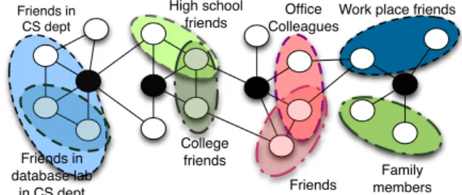
up-High school friends Family members Office Colleagues Friends College friends Friends in database lab in CS dept Friends in CS dept
Work place friends
Fig. 1 An example of neighborhood-centric analysis: identify users’
social circlesin a social network.
date the states maintained in the vertices. Any multi-hop traversal in X-Stream would be expensive as it requires mul-tiple iterations of the scatter, shuffle and gather phases. Since the stream partitioning used by the framework does not take the neighborhood structure into account, such operations would necessitate a large amount of data to be shuffled to the gather phase across different stream partitions. X-Stream also fun-damentally relies on the vertex state remaining constant in size, and it would negate the key benefits of X-Stream if variable-sized neighborhoods were constructed in the vertex state. Finally, X-Stream provides a restricted edge-centric API that would make it hard to encode neighborhood-centric computations such as those supported by NSCALE.
GraphX, built on top of Apache Spark, supports a flexi-ble set of operations on large graphs [16]; however, GraphX stores the vertex information and edge information as sep-arate RDDs, which necessitates a join operation for each edge traversal. Further, the only way to support subgraph-centric operations in GraphX is through its emulation of the vertex-centric programming framework, and our experimen-tal comparisons with GraphX show that it suffers from the same limitations of the vertex-centric frameworks as dis-cussed above.
3 Application Scenarios
This section discusses several representative graph analytics tasks that are ill-suited for vertex-centric frameworks, but fit well with NSCALE’s subgraph-centric computation model. Local clustering coefficient (LCC). In a social network, the LCC quantifies, for a user, the fraction of his or her friends who are also friends—this is an important starting point for many graph analytics tasks. Computing the LCC for a vertex requires constructing its ego network, which includes the vertex, its 1-hop neighbors, and all the edges between the neighbors. Even for this simple task, the limi-tations of vertex-centric approaches are apparent, since they require multiple iterations to collect the ego-network before performing the LCC computation (such approaches quickly run out of memory as we increase the number of vertices we are interested in).
V2 V1 V3 V2 V1 V3 V1 V2 V3 V4 (a) (b) (c)
Fig. 2 Counting different types of network motifs: (a) Feed-fwd Loop,
(b) Feedback Loop, (c) Bi-parallel Motif.
Identifying social circles.Given a user’s social network (k-hop neighborhood), the goal is to identify the social circles (subsets of the user’s friends), which provide the basis for information dissemination and other tasks. Current social networks either do this manually, which is time consuming, or group friends based on common attributes, which fails to capture the individual aspects of the user’s communities. Figure 1 shows examples of different social circles in the ego networks of a subset of the vertices (i.e., shaded vertices). Automatic identification of social circles can be formulated as a clustering problem in the user’sk-hop neighborhood, for example, based on a set of densely connected alters [31]. Once again, vertex-centric approaches are not amenable to algorithms that consider subgraphs as primitives, both from the point of view of performance and ease of programming. Counting network motifs.Network motifs are subgraphs that appear in complex networks (Figure 2), which have im-portant applications in biological networks and other do-mains. However, counting network motifs over large graphs is quite challenging [23] as it involves identifying and count-ing subgraph patterns in the neighborhood of every query vertex that the user is interested in. Once again, in a vertex-centric framework, this would entail message passing to gather neighborhood data at each vertex, incurring huge messaging and memory overheads.
Social recommendations.Random walks with restarts (such as personalized PageRank [9]) lie at the core of several so-cial recommendation algorithms. These algorithms can be implemented using Monte-Carlo methods [18] where the random walk starts at a vertexv, and repeatedly chooses a random outgoing edge and updates a visit counter with the restriction that the walk jumps back only to v with a cer-tain probability. The stationary distribution of such a walk assigns a PageRank score to each vertex in the neighbor-hood ofv; these provide the basis for link prediction and rec-ommendation algorithms. Implementing random walks in a vertex-centric framework would involve one iteration with message passing for each step of the random walk. In con-trast, with NSCALEthe complete state of thek-hop neigh-borhood around a vertex is available to the user’s program, which can then directly execute personalized PageRank or any existing algorithm of choice.
Subgraph Pattern Matching and Isomorphism.Subgraph pattern matching or subgraph isomorphism have important
applications in a variety of application domains including biological networks, chemical interaction networks, social networks, and many others; and a wide variety of techniques have been developed for exact or approximate subgraph pat-tern matching [46, 52, 12, 53, 54, 50, 36, 45, 19, 49, 33] (see Lee et al. [26] for a recent comparison of the state-of-the-art techniques). Many of those techinques work by identify-ing potential matches for a central node in the pattern, and then exploring the neighborhood around those nodes to look for matches. This second step can often involve fairly so-phisticated algorithms, especially if the patterns are large or contain sophisticated constructs, or if the goal is to find ap-proximate matches, or if the data is uncertain. Most of those algorithms are not easily parallelizable, and hence it would not be easy to execute them in a distributed fashion using the vertex-centric programming frameworks. On the other hand, NSCALE could be used to construct the relevant neighbor-hoods in memory in many of those cases, and those search algorithms could be used as is on those neighborhoods.
4 NScale Overview 4.1 Programming Model
We assume a standard definition of a graphG(V, E)where
V = {v1, v2, ..., vn} denotes the set of vertices and E =
{e1, e2, ..., em} denotes the set of edges in G. Let A =
{a1, a2, ..., ak} denote the union of the sets of attributes
associated with the vertices and edges inG. In contrast to vertex-centric programming models, NSCALEallows users to specify subgraphs or neighborhoods as the scope of com-putation. More specifically, users need to specify: (a) sub-graphs of interest on which to run the computations through asubgraph extraction query, and (b) a user program. Specifying subgraphs of interest.We envision that NSCALE will support a wide range of subgraph extraction queries, in-cluding pre-defined parameterized queries, and declaratively specified queries using a Datalog-based language that we are currently developing. Currently, we support extraction queries that are specified in terms of four parameters: (1) a predicate on vertex attributes that identifies a set ofquery vertices(PQV), (2)k– the radius of the subgraphs of
inter-est, (3) edge and vertex predicates to select a subset of ver-tices and edges from thosek-hop neighborhoods (PE, PV),
and (4) a list of edge and vertex attributes that are of interest (AE, AV). This captures a large number of subgraph-centric
graph analysis tasks, including all of the tasks discussed ear-lier. For a given subgraph extraction queryq, we denote the subgraphs of interest bySG1(V1, E1), ..., SGq(Vq, Eq).
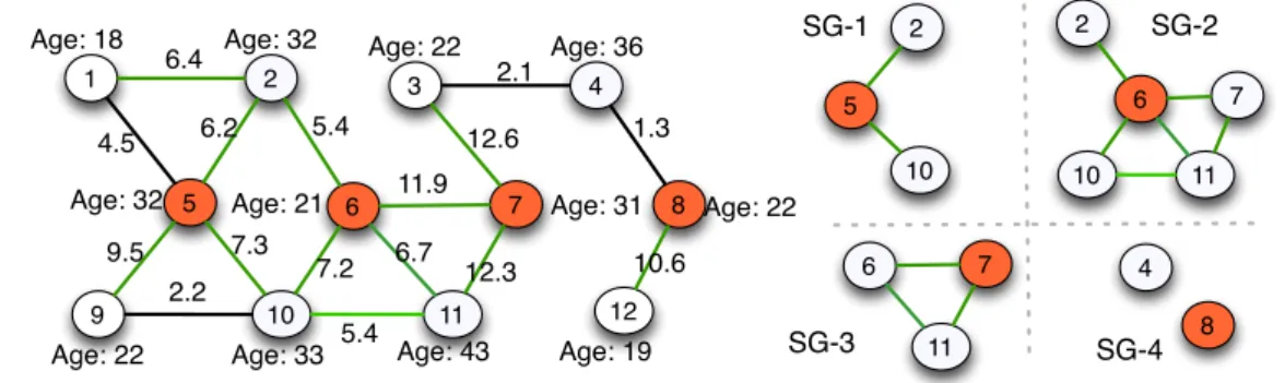
Figure 3 shows an example subgraph extraction query, where the query vertices are selected to be vertices with
age >18, radius is set to 1, and the user is interested in
ex-ArrayList<RVertex> n_arr = new ex-ArrayList<RVertex>(); for(Edge e: this.getQueryVertex().getOutEdges)
n_arr.add(e.getVertex(Direction.IN));
int possibleLinks = n_arr.size()* (n_arr.size()-1)/2; // compute #actual edges among the neighbors
for(int i=0; i < n_arr.size()-1; i++) for(int j=i+1; j < n_arr.size(); j++)
if(edgeExists(n_arr.get(i), n_arr.get(j))) numEdges++;
double lcc = (double) numEdges/possibleLinks;
Fig. 4 Example user program to computelocal clustering coefficient
written using the BluePrints API. TheedgeExists()call requires access to neighbors’ states, and thus this program cannot be executed as is in a vertex-centric framework.
tracting induced subgraphs containing vertices withage > 25 and edges with weight > 5. The four extracted sub-graphs,SG1, ..., SG4are also shown.
Specifying subgraph computation user program.The user computation to be run against the subgraphs is specified as a Java program against the BluePrints API [2], a collection of interfaces analogous to JDBC but for graph data. Blueprints is a generic graph Java API used by many graph process-ing and programmprocess-ing frameworks (e.g., Gremlin, a graph traversal language [4]; Furnace, a graph algorithms pack-age [3]; etc.). By supporting the Blueprints API, we imme-diately enable use of many of these already existing toolk-its over large graphs. Figure 4 shows a sample code snip-pet of how a user can write a simple local clustering coeffi-cient computation using the BluePrints API. The subgraphs of interest here are the 1-hop neighborhoods of all vertices (by definition, a 1-hop neighborhood includes the edges be-tween the neighbors of the node).
NSCALEsupports the Bulk Synchronous Protocol (BSP) for iterative execution, where the analysis task is executed using a number of iterations (also calledsupersteps). In each iteration, the user program is independently executed in par-allel on all the subgraphs (in a distributed fashion). The user program may then change the state of the query vertex on which it is operating (for consistent and deterministic se-mantics, we only allow the user program to change state of the query vertex that it owns; otherwise we would need a mechanism to arbitrate conflicting changes to a vertex state and we are not aware of any clean and easy model for achiev-ing that). The state changes are made visible across all the subgraphs during the synchronization barrier, through use of shared state for subgraphs on the same partition and through message passing for subgraphs on different partitions. We provide a more detailed description of the provision of sup-port for iterative computation in NSCALE, including the con-sistency and ownership model used, in Section 6.3.
Certain user applications might require customized ag-gregation of the values produced as a result of executing
1 5 2 9 10 3 7 4 11 12 6 8 6.2 4.5 7.3 9.5 2.2 5.4 7.2 11.9 12.3 12.6 2.1 1.3 10.6 6.4
Age: 18 Age: 32 Age: 22 Age: 36
Age: 19 Age: 22 Age: 31 Age: 43 Age: 33 Age: 22 Age: 32 Age: 21 6.7 5.4
Subgraph Extraction Query: {Node.Sex = Male; Node.age > 18}, 1, {{Node.age > 25}, {Edge.weight > 5}}, all
5 2 10 2 10 7 11 6 4 8 7 11 6 SG-1 SG-2 SG-3 SG-4
Fig. 3 A subgraph extraction query on a social network
the user-specified program on the subgraphs of interest. Our mechanism to handle state updates for iterative tasks can also be used for aggregating information across all the nodes in the graph in the synchronization step. To briefly summa-rize, the nodes can send messages to the coordinator that it can use to make various decisions (e.g., when to stop). The messages can be first locally aggregated, and the final aggregation is done by the coordinator (depending on the aggregation function).
4.2 System Architecture
Figure 5 shows the overall system architecture of NSCALE, which is implemented as a Hadoop YARN application. The framework supports ingestion of the underlying graph in a variety of different formats including edge lists, adjacency lists, and in a variety of different types of persistent stor-age engines including key–value pairs, specialized indexes stored in flat files, relational databases, etc. The two major components of NSCALEare the graph extraction and pack-ing (GEP) module and the distributed execution engine. We briefly discuss the key functionalities of these two compo-nents here, and present details in the following sections. Graph Extraction and Packing (GEP) Module.The user specifies the subgraphs of interest and the graph computa-tion to be executed on them using the NSCALE user API. Unlike prior graph processing frameworks, the GEP mod-ule forms a major component of the overall NSCALE frame-work. From a usability perspective, it is important to provide the ability to read the underlying graph from the persistent storage engines that are not naturally graph-oriented. How-ever, more importantly, partitioning and replication of the graph data are more critical for graph analytics than for an-alytics on, say, relational or text data.
Graph analytics tasks, by their very nature, tend to tra-verse graphs in an arbitrary and unpredictable manner. If the graph is partitioned across a set of machines, then many of
these traversals are made over the network, incurring signif-icant performance penalties. Further, as the number of par-titions of a graph grows, the number ofcutedges (with end-points in different partitions), and hence the number of dis-tributed traversals, grows in a non-linear fashion. This is in contrast to relational or text analytics where the number of machines used has a minor impact on the execution cost.
This is especially an issue in NSCALE, where user pro-grams are treated as black-boxes. Hence, we have made a design decision to avoid distributed traversals altogether by replicating vertices and edges sufficiently so that every sub-graph of interest is fully present in at least one partition. Similar approach has been taken by some of the prior work on efficiently executing “fetch neighbors” queries [38] and SPARQL queries [21] in distributed settings. The GEP mod-ule is used to ensure this property, and is responsible for ex-tracting the subgraphs of interest and packing them onto a small set of partitions such that every subgraph of interest is fully contained within at least one partition. GEP is im-plemented as multiple MapReduce jobs (described in detail later). The output is avertex-to-partition mapping, which consists of a mapping from the graph vertices to partitions to be created. This data is either written to HDFS or directly fed to the execution engine.
Distributed Execution Engine.The distributed execution phase in NSCALEis implemented as a MapReduce job, which reads the original graph and the mappings generated by GEP, shuffles graph data onto a set of reducers, each of which constructs one of the partitions. Inside each reducer, the ex-ecution engine is instantiated along with the user program, which then receives and processes the graph partition.
The execution engine supports both serial and parallel execution modes for executing user programs on the ex-tracted subgraphs. For serial execution, the execution engine uses a single thread and loops across all the subgraphs in a partition, whereas for parallel execution, it uses a pool of threads to execute the user computation in parallel on multi-ple subgraphs in the partition. However, this is not
straight-HDFS Subgraph Extraction
Cost Based Optimizer
Set Bin Packing
Map Phase
Reducer 1 Reducer N Node to
Bin mapping Underlying Graph Data
Flat Files K-V Stores Special Purpose Indexes
NScale User API
Graph Extraction and Packing Distributed Execution Engine
Apache YARN Map Reduce Output Materialization Exec Engine Exec Engine
Fig. 5 NSCALEarchitecture. The GEP module is responsible for
ex-tracting and packing subgraphs of interest and then handing off the partitions to the distributed execution engine.
forward because the different subgraphs of interest in a par-tition are stored in an overlapping fashion in memory to re-duce the total memory requirements. The execution engine employs several bitmap-based techniques to ensure correct-ness in that scenario.
5 Graph Extraction and Packing 5.1 Subgraph Extraction
Subgraph extraction in the GEP module has been imple-mented as a set of MapReduce (MR) jobs. The number of MR stages needed depends on the size of the graph, how the graph is laid out, size(s) of the machine(s) available to do the extraction, and the complexity of the subgraph extraction query itself. The first stage of GEP is always a map stage that reads in the underlying graph data, and identifies thequery vertices. It also applies the filtering predicates (PE, PV) to
remove the vertices and edges that do not pass the predi-cates. It also computes asizeorweightfor each vertex, that indicates how much memory is needed to hold the vertex, its edges, and their attributes in a partition. This allows us to estimate the memory required by a subgraph as the sum of the weights of its constituent vertices. (Only the attributes identified in the extraction query are used to compute these weights.) The rest of the GEP process only operates upon the network structure (the vertices and the edges), and the vertex weights.
Case 1: Filtered graph structure is small enough to fit in a single machine.In that case, the vertices, their weights, and their edges are sent to a single reducer. That reducer constructs the subgraphs of interest and represents them as subsets of vertices, i.e., each subgraph is represented as a list of vertices along with their weights (no edge informa-tion is retained further); this is sufficient for the subgraph packing purposes. The subgraph packing algorithm takes as input these subsets of vertices and the vertex weights, and produces a vertex-to-partition mapping.
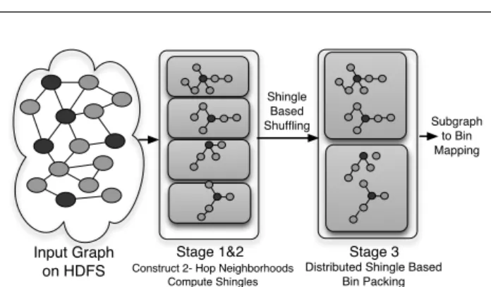
Input Graph on HDFS
Stage 1&2 Construct 2- Hop Neighborhoods
Compute Shingles
Stage 3
Distributed Shingle Based Bin Packing Shingle Based Shuffling Subgraph to Bin Mapping
Fig. 6 Distributed GEP Architecture: Stages 1 and 2 construct the
2-hop neighborhoods; Stage 3 does the distributed shingle based bin packing producing the final subgraph to bin mapping.
Case 2: Filtered graph structure does not fit on a single machine.In that case, the subgraph extraction and packing both are done in a distributed fashion, with the number of stages dependent on the radius (k) of subgraphs of inter-est. We explain the process assumingk= 2, i.e., assuming our subgraphs of interest are 2-hop neighborhoods around a set of query vertices. We also assume an adjacency list rep-resentation of the data1 (i.e., the IDs of the neighbors of a
vertex are stored along with rest of its attributes);
Figure 6 shows the 3-stage distributed architecture of GEP. We begin with providing a brief sketch of the process. Given an input graph and a user query, the first two stages es-sentially are responsible for gathering for each query-vertex, its 2 hop neighborhood along with the weight attributes as-sociated with each vertex in the 2-hop neighborhood. This is done iteratively, wherein the first stage constructs the 1-hop neighborhood of the query-vertices specified by the query with all the required information on a set of reducers. Sub-sequently, the second stage takes the output of the first stage as input, constructs the 2-hop neighborhoods of the query-vertices and computes their shingle values in a distributed fashion, and outputs them as keys associated with these query-vertex neighborhoods. The final stage shuffles the neighbor-hoods based on these keys to multiple reducers in an attempt to group together neighborhoods with high overlap on a sin-gle reducer. The reducers in stage 3 run the bin packing in parallel which is followed by a post-processing step to pro-duce the final neighborhood-to-bin mapping.
Next, we provide an in-depth description of the process. For a nodeu, letN(u) =u1, ..., uN(u)denote its neighbors.
The following steps are taken:
MapReduce Stage 1:For each vertexuthat passes the fil-tering predicates (PV), the map stage emitsN(u)+1records:
hkey,(u, weight(u), isQueryV ertex, N(u))i,
wherekey = u, u1, ..., uN(u). Thus, given a vertex u, we
haveN(u)0+ 1records that were emitted withuas the key, 1 For input graphs represented as an edge list with the vertex at-tributes available as a separate mapping, we have a minor modification to the first stage that uses a MapReduce job to join the edge and vertex data and produce a distributed adjacency list in the required format.
one for its own information, and one for each of itsN(u)0 neighbors that satisfiesPV (emitted while those neighbors
are processed). In the reduce stage, the reducer responsible for vertexunow has all the information for its 1-hop neigh-bors, and IDs of all its 2-hop neighbors (obtained from its neighbors’ neighborhoods), but it does not have the weights of its 2-hop neighbors or whether they satisfied the filter-ing predicatesPV. For each query vertexu, the reducer
cre-ates a list of the nodes in its 2-hop neighborhood, and out-puts that information with key u. For each vertex v and for each of its 2-hop neighbors w, it also emits a record
hkey=w,(v, weight(v))i.
MapReduce Stage 2:The second MapReduce stage groups the outputs of the first MapReduce stage by the vertex ID. Each reducer processes a subset of the vertices. There are two types of records that a reducer might process for a vertex
u: (a) a record containing a list ofu’s 1- and 2-hop
neigh-bors and the weights of its 1-hop neighneigh-bors, and (b) several records each containing the weight of a 2-hop neighbor ofu. If a reducer only sees the records of the second type, thenu is not a query vertex, and those records are discarded. Oth-erwise, the reducer adds the weight information for 2-hop neighbors, and completes the subgraph corresponding tou. For each of the subgraphs, the reducer then computes a min-hash signature, i.e., a set ofshingles, over the vertex set of the subgraph, and emits a record with the set of shingles as the key and the subgraph as the value (we use 4 shingles in our experiments). A shingle is computed by applying a hash function to each of the vertex IDs in the subgraph, and tak-ing the minimum of the hash values; it is well known that if two sets share a large fraction of the shingles, then they are likely to have a high overlap [40].
MapReduce Stage 3:The third MapReduce phase uses the shingle value of the subgraphs to shuffle the subgraphs to appropriate reducers. As a result of this shuffling, the sub-graphs that are assigned to a reducer are likely to have high overlap and the subgraph packing algorithm is executed on each reducer separately. Finally, a post-processing step com-bines the results of all the reducers by merging any partitions that might be underutilized in the solutions produced by the individual reducers.
Intuitively, the above sequence of MapReduce stages con-structs the required subgraphs, and then does a shuffle using the shingles technique in an attempt to create groups that contain overlapping subgraphs. Those groups are then pro-cessed independently and the resulting vertex-to-partition mappings are concatenated together.
5.2 Subgraph Packing
Problem Definition. We now formally define the problem of packing the extracted subgraphs into a minimum number
of partitions (or bins)2, such that each subgraph is contained
within a partition and the computation load across the parti-tions is balanced. LetSG={SG1, SG2, .., SGq}be the set
of subgraphs extracted from the underlying graph data (at a reducer). As discussed earlier, we assume that the memory required to hold a subgraphSGican be estimated as the sum
of weights of the nodes in it. LetBCdenote the bin capacity. This is set based on the maximum container capability of a YARN cluster node, a configuration parameter that needs to be set for the YARN cluster keeping in mind the maximum allocation of resources to individual tasks on the cluster
Without considering overlaps between subgraphs and the load balancing objective, this problem reduces to the stan-dardbin packing problem, where the goal is to minimize the number of bins required to pack a given set of objects. The variation of the problem where the objects aresets, and when packing multiple such objects into a bin, aset unionis taken (i.e., overlaps are exploited), has been calledset bin packing; that problem is considered much harder and we have found very little prior work on that problem [22].
Further, we note that we have a dual-objective optimiza-tion problem; we reduce it to a single-objective optimizaoptimiza-tion problem by putting a constraint on the number of subgraphs that can be assigned to a bin. LetM AX denote the con-straint, i.e., the maximum number of subgraphs that can be assigned to a bin.
Subgraph Bin Packing Algorithms. The subgraph bin packing problem is NP-Hard and appears to be much harder to solve than the standardbin packingproblem, as it also exhibits some of the features of theset coverand thegraph partitioningproblems. Next, we develop several scalable heuris-tics to solve this problem. We also developed and imple-mented an optimal algorithm for this problem (OPT), where we construct an Integer Program for the given problem in-stance and use the Gurobi Optimizer to solve the Integer Program. We were, however, able to run OPT successfully only for a very few small graphs; we present those results in Section 8.2.
5.2.1 Bin Packing-based Algorithms
The first set of heuristics that we develop exploit the similar-ity between subgraph packing problem and the bin packing problem. All of these heuristics use the standard greedy bin packing algorithm, where the items are considered in a par-ticular order and placed in the first bin where they fit. More specifically, the algorithm (Algorithm 1) takes as input an ordered list of subgraphs, as determined by the heuristic, processes them in order, and packs each subgraph into the first available bin that has the available residual capacity, without violating the constraint on the maximum number of subgraphs in a bin. The addition of a subgraph to a bin is 2 We use the termspartitionsandbinsinterchangeably in this paper.
a set union operation that takes care of the overlap between the subgraphs. Each bin represents a partition onto which the actual graph data, associated with the nodes mapped to the bin using this algorithm, would be distributed for final execution step.
The complexity of this algorithm in the worst case in terms of the number of comparison operations required is O(nm)wherenis the number of subgraphs andmis the number of bins required (=nin the worst case). Each com-parison operation compares the estimated size of the union (accounting for the overlap) and the bin capacity. In addi-tion to these comparisons, there would benset union oper-ations for inserting the subgraphs into bins. The complexity of the comparison and the set union operations is implemen-tation dependent. For a hashtable-based approach, those op-erations would be linear in the number of set elements, giv-ing us an overall complexity ofO(nmC), where C is the bin capacity. However this worst-case complexity is quite pessimistic, and in practice, the algorithms run very fast.
We now describe three different heuristics to provide the input ordering of the subgraphs to be packed into bins.
Algorithm 1:Bin Packing Algorithm.
Input : Ordered list of subgraphsSG1, ..., SGq, each
represented as a list of vertices and edges
Input : Bin capacityBC; Maximum number of subgraphs per
binM AX
Output: Partitions
fori= 1,2, ..., qdo
forj= 1,2, ..., Bdo
ifnumber of subgraphs in Bin j<MAXthen ifSGifits in Binj(accounting for overlap)then
AddSGito Binj; break;
end end end
ifSGinot yet placed in a binthen Create a new bin and addSGito it; end
end
1. First Fit bin packing algorithm. The first fit algo-rithm is a standard greedy 2-approximation algoalgo-rithm for bin packing, and processes the subgraphs in the order in which they were received (i.e., in arbitrary order).
2. First Fit Decreasing bin packing algorithm. The first fit decreasing algorithm is a variant of the first fit algorithm wherein the subgraphs are considered in the decreasing or-der of their sizes.
3. Shingle-based bin packing algorithm. The key idea be-hind this heuristic is to order the subgraphs with respect to the similarity of their vertex sets. The ordering so produced will maximize the probability that subgraphs with high
over-lap are processed together, potentially resulting in a better overall packing.
The shingle-based ordering is based on the min-hashing technique [39] which produces signatures for large sets that can be used to estimate the similarity of the sets. For com-puting themin-hashsignatures (or shingles) of the subgraphs of interest over their vertex set, we choose a set ofk differ-ent random hash functions to simulate the effect of choos-ingkrandom permutations of the characteristic matrix that represents the subgraphs. For each query vertex and each hash function, we apply the hash function to the set of nodes in the subgraph of the query vertex and find the minimum among the hash values.
Thus the output of the shingle computation algorithm (Ref Algorithm 2) is a list ofkshingles (min-hash values) for each subgraph of interest, where the order of the hash functions within the list is effectively arbitrary3. To com-pute the shingle ordering, we sort-order the subgraphs of interest based on this list of shingle values associated with the subgraphs in a lexicographical fashion. The sorted or-der so obtained using this technique places subgraphs with high Jaccard similarity (i.e., overlap) in close proximity to each other. This shingle-based order is then used to pack the neighborhoods into bins using the greedy algorithm. Handling skew.A high variance in the sizes of subgraphs could lead to a bin packing where some partitions have only a few large subgraphs and few partitions have a very large number of small subgraphs. This might lead to load imbal-ance and skewed execution times across partitions. To han-dle this skew in the sizes of the subgraphs, the bin packing algorithm (Algorithm 1) accepts a constraint on the maxi-mum number of subgraphs (MAX) in a bin in addition to the bin capacity. This limits the number of small subgraphs that can be binned together in a partition and mitigates the po-tential of load imbalance between partitions to some degree. The trade-off here is that, we may need to use a higher num-ber of bins to satisfy the constraints while some of the bins are not fully utilized. The MAX parameter can be set em-pirically depending on the nature of user computation and the underlying graph keeping in view the above mentioned trade-off.
5.2.2 Graph Partitioning-based Algorithms
The subgraph packing problem has some similarities to the graph partitioningproblem, with the key difference being that: standard graph partitioning problem asks for disjoint balanced partitions, whereas the partitions that we need to create typically have overlap in order to satisfy the require-ment that each subgraph be completely contained within at 3 The higher the value ofk, the better the quality of the result. We have chosenk = 6for our implementation which was determined experimentally to strike a fine balance between the quality of shingle-based similarity and computation time.
Algorithm 2:Computing shingles for a subgraph
Input : SubgraphSG(V, E); A family of
pairwise-independent hash functionsH
shingles[SGi]← {};
forh∈Hdo
shingles[SG]← {shingles[SG], minv∈Vh(v)};
end
returnshingles;
least one partition. Graph partitioning is very well-studied and a number of packages are available that can partition large graphs efficiently, METIS perhaps being the most widely used [5].
Despite the similarities, graph partitioning algorithms turn out to be a bad fit for the subgraph packing problem, because it is not easy to enforce the constraint that each subgraph of interest be completely contained in a partition. One option is to start with a disjoint partitioning returned by a graph par-titioning algorithm, and then “grow” each of the partitions to ensure that constraint. However, we also need to ensure that the enlarged partitions obey the bin capacity constraint, which is hard to achieve since different partitions may get enlarged by different amounts.
We instead take the following approach (Algorithm 3). Weoverpartitionthe graph using a standard graph partition-ing algorithm (we use METIS in our implementation) into a large number of fine-grained partitions. We then grow each of those partitions as needed. This requires that for each query vertex in the fine grained partition, we check is its k-hop neighborhood lies within the partition. If not, we repli-cate the required nodes in the partition. This ensures that each subgraph of interest is fully contained in one of the par-titions, and finally use the shingle-based bin packing heuris-tic to pack those partitions into bins. While packing, we also keep track of the nodes that are owned by the bin (or par-tition) and the ones that are replicated (ghosts) from other bins, to maintain the invariant of keeping each subgraph of interest fully in the memory of one of the partitions.
5.2.3 Clustering-based Algorithms
The subgraph packing problem also has similarities to clus-tering, since our goal can be seen as identifying similar (i.e., overlapping) subgraphs and grouping them together into bins. We developed two heuristics based on the two commonly used clustering techniques.
Agglomerative Clustering-based Algorithm. Agglomer-ative clustering refers to a class of bottom-up algorithms that start with each item being in its own cluster, and re-cursively merge the closest clusters till the requisite number of clusters is reached. For handling large volumes of data, a threshold-based approach is typically used where in each step, pairs of clusters that are sufficiently close to each other
Algorithm 3:Graph Partitioning-based algorithm.
Input : GraphG(V, E); Num of over partitionsk
Output: BinsB
//Over partitionGintokpartitions.;
P ←Metis(G); where|P|=k;
forp∈Pdo
forqv∈pdo
if !(k−hop neighborhood)∈pthen
Grow: Replicate the required nodes adding them top;
end end end
//Compute Shingles for each grown partition; fori = 1 to|P|do
si=ComputeShingles(pi);
end
//Sort the partitions based on shingle values (si) ; Sort(P);
B=BinP ackingAlgo(P);
returnB;
are merged, and the threshold is slowly increased. Next we sketch our adaptation of this technique to subgraph packing. We start with computing a set of shingles for each sub-graph and ordering the subsub-graphs in the shingle order. This is done in order to reduce the number of pairs of clusters that we consider for merging; in other words, we only consider those pairs for merging that are sufficiently close to each other in the shingle order. The functioncreateAggClusters() in Algorithm 4 does the actual scanning of sets and merges close by sets together. The algorithm uses two parameters, both of which are adapted during the execution: (1) τ, a threshold that controls when we merge clusters, and (2)l, that controls how many pairs of clusters we consider for merging. In other words, we only merge a pair of clusters if they are less thanlapart in the shingle order, and the Jac-card distance between them is less thanτ. The set of merged clusters are available asAC.
To reduce the number of parameters, we use a sampling-based approach in the functionsetT hreshold()in Algo-rithm 4, to setτat the beginning of each iteration. We choose a random sample of the eligible pairs (we use 1% sample), compute the Jaccard distance for each pair, and setτ such that 10% of those pairs of clusters would have distances be-lowτ. We experimented with different percentage thresh-olds, and we observed that 10% gave us the best mix of quality and running time.
After computingτ, we make a linear scan over the clus-ters that have been constructed so far. For each cluster, we compute its actual Jaccard distance with thel clusters that follow it. If the smallest of those distances is less thanτ, then we merge the two clusters and re-compute shingles for the merged cluster (this is done by simply picking the min-imum of the two values for each shingle position). This is
Algorithm 4: Agglomerative Clustering-based algo-rithm.
Input : Set of subgraphsSG={SG1, ..., SGq}
Input : Merge sizel(Number of pairs to be considered for
merging.)
Output: Agglomerative Clusters (Bins)AC
//Compute Shingles of each subgraph;
fori= 1toqdo
si=ComputeShingles(SGi);
end
/*Sort the subgraphs based on their shingle values
(S={s1, s2, ..sq})*/;
Sort(SG) ; Done=false;
//Create an empty set of agglomerative clusters;
AC ←φ;
while!Donedo
τ= setThreshold();
numM erges=createAggCluster(SG,AC, τ, I);
ifnumM erges= 0then
Done=True; break; end
//adjust the merge size if required;
I= adjustMergeSize();
//Re-Compute Shingles of each merged cluster;
m=|AC|;
fori= 1tomdo
si=ComputeShingles(ACi);
end
//Sort clusters based on their shingle values (si). Sort(AC) ;
SG=AC;
end
returnAC;
only done if the merged cluster does not exceed the bin ca-pacity (pairs of clusters whose union exceeds bin caca-pacity are also excluded from the computation ofτ).
During computation ofτ, we also keep track of the num-ber of pairs excluded because the size of their union is larger than the bin capacity. If those pairs form more 50% of sam-pled pairs, then we increasel(adjustM ergeSize()) to in-crease the pool of eligible pairs. Since this usually happens towards the end when the number of clusters is small, we do this aggressively by increasinglby 50% each time. The algorithm halts when it cannot merge any pair of clusters without violating the bin capacity constraint.
K-Means-based Algorithm.K-Means is perhaps the most commonly used algorithm for clustering, and is known for its scalability and for constructing good quality clusters. Our adaptation of K-means (Ref Algorithm 5) is sketched next.
We start by pickingkof the subgraphs randomly as cen-troids. We then make a linear scan over the subgraphs and for each subgraph, we compute the distance to each centroid using the functioncomputeDistance(). We assign the sub-graph to the centroid with which it has the highest intersec-tion (in other words, we assign it to the centroid whose size
Algorithm 5:KMeans Clustering-based algorithm.
Input : Set of subgraphsSG={SG1, ..., SGq}; Bin
CapacityBC
Input :k: The number of K-Means Clusters; MAX:
maximum iterations
Output: BinsB
//Create an empty centroid setKC ←φ;
//Randomly pick k subgraphs and assign them as the k-centroids;
while(Sizeof(KC)< k)do
//Generate a random number from 1 to k i=GenerateRandom(k);
KC=KCSSG
i end
//Scan over the set of subgraphs and assign them to nearest centroid; AssignmentM ap←φ; fori = 1 to qdo if!(SGi∈ KC)then Max =−∞; CentroidAssigned =0; forj=1 to kdo dist =computeDistance(SGi, KCj, BC); if(M ax < dist)then Max = dist; CentroidAssigned = j; end end UpdateCentroid(SGi, KCCentroidAssigned); AssignmentMap.Put(i,CentroidAssigned); end end
//Update assignments iteratively to improve clustering; numIterations=0; whilenumIterations < M AXdo fori = to qdo CurrentAssignment = AssignmentMap.Get(i); forj = 1 to kdo SwapGain = ComputeGain(i, CurrentAssignment, j); if(SwapGain >0)then Swap(i, CurrentAssignment, j); end end end numIterations++; end B=BinP ackingAlgo(KC); returnB;
needs to increase the least to include the subgraph). This is only done if the total size of the vertices in the cluster does not exceed BC. After assigning the subgraph to the cen-troid, we recompute the centroid (U pdateCentroid()) as the union of the old centroid and the subgraph. The function also keeps track of multiplicities of the vertices in the cen-troid at all times (i.e., for each vertex in a cencen-troid, we keep track of how many of the assigned subgraphs contain it).
As with K-Means, we make repeated passes over the list of subgraphs in order to improve the clustering. In the
sub-Algorithm 6:ComputeDistance()
Input : SubgraphSG; CentroidC; Bin CapacityBC
Output: Distance betweenSGandC
if|SG∪C|> BCthen
return-∞
else
return|SG∩C|
end
sequent iterations, for each subgraph, we check if it may improve the solution using the function ComputeGain(). If the swap gain is positive, i.e. there is a net decrease in the sum of the size of the centroids involved in the swap, we reassign the subgraph to a different centroid, using the mul-tiplicities to remove it from one centroid and assign it to the other centroid (Swap()). Finally the k cluster obtained are packed into bins (or partitions).
Having to choose a value ofka priori is one of the key disadvantages of K-Means. We estimate a value ofkbased on the subgraph sizes and the bin capacity. If at the end of first iteration, we discover that we are left with too many unassigned subgraphs, we increase the value ofkand repeat the process till we are able to find a good clustering.
5.3 Handling Very Large Subgraphs
Most machines today, even commodity machines, have large amounts of RAM available, and can easily handle very large subgraphs, including 2-hop neighborhoods of high-degree nodes in large-scale networks. However, in the rare case of a subgraph extraction query where one of the subgraphs ex-tracted is too large to fit into the memory of a single ma-chine, we have two options. The first option is to use disk-resident processing, by storing the subgraph on the disk and loading it into memory as needed. The user program may need to be modified so that it does not thrash in such a sce-nario. We note here that our flexible programming model makes it difficult to process the subgraph in a distributed fashion (i.e., by partitioning the subgraph across a set of distributed machines); if this scenario is common, we may wish to enforce a vertex-centric programming model within NSCALE, and that is something we plan to consider in future work.
The other option, that we currently support in NSCALE and is arguably better suited for handling large subgraphs, is to use samplingto reduce the size of the subgraph. We currently assume that the subgraph skeleton (i.e., the net-work structure of a subgraph) can be held in the memory of a single machine during GEP; this is needed to support many of the effective random sampling techniques like for-est fire or random walks (independent random sampling can be used without making this assumption) [27], [37]. The
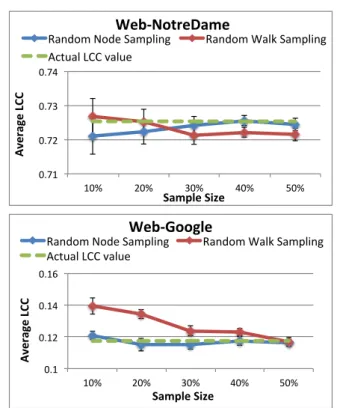
0.71 0.72 0.73 0.74 10% 20% 30% 40% 50% Av er ag e LC C Sample Size
Web-‐NotreDame
Random Node Sampling Random Walk Sampling
Actual LCC value 0.1 0.12 0.14 0.16 10% 20% 30% 40% 50% Av er ag e LC C Sample Size
Web-‐Google
Random Node Sampling Random Walk Sampling Actual LCC value
Fig. 7 Effect of Graph Sampling
key idea here is to construct a random sample of a sub-graph during GEP, if the size of the subsub-graph is estimated to be larger than the bin capacity. We provide built-in sup-port for two random sampling techniques:random node se-lection, andrandom walk-based sampling. The former tech-nique chooses an independent random sample of the nodes to be part of the subgraph, whereas the latter technique does random walks starting with the query vertex and including all visited nodes in the sample (till a desired sample size is reached). NSCALEalso provides a flexible API for users to implement and provide their own graph sampling/compression technique. The random sampling is performed at the reduce stage in GEP where the subgraph skeleton is first constructed.
Figure 7 shows the effect of using our random node and random walk-based sampling algorithms on the accuracy of the local clustering coefficient (LCC) computation. We plot the average LCC computed on samples of different sizes for two different data sets, and compare them to the actual re-sult. Each data point is an average of 10 runs. We also show the standard deviation error bars. For the random node-based sampling techniques, the standard deviation across multi-ple random runs decreases and the accuracy increases as the sampling ratio increases (as seen in that figure). This is not surprising since the estimated LCC through this technique is an unbiased estimator for the true average LCC (although it has a very high variance). For the random walk-based sam-pling, the numbers do not show any consistent trend since the set of sampled nodes does not have any uniformity guar-antees and in fact, the set of sampled nodes would be biased towards the high degree nodes (and the effect on the
esti-mated LCC would be arbitrary since the degree of a node is not directly correlated with the LCC for that node).
6 Distributed Execution Engine
The NSCALE distributed execution engine runs inside the reduce stage of a MapReduce job (Figure 5). The map stage takes as input the original graph and the vertex-to-partition mappings that are computed by the GEP module, and it repli-cates and shuffles the graph data so that each of the re-ducers gets the data corresponding to one of the partitions. Each reducer constructs the graph in memory from the data that it receives, and identifies the subgraphs owned by it (the vertex-to-partition mappings contain this information as well). It then uses a worker thread pool to execute the user computation on those subgraphs. The output of the graph computation is written to HDFS.
6.1 Execution modes
The execution engine provides several different execution modes. Thevector bitmap modeassociates a bit-vector with each vertex and edge in the partition graph, and enables par-allel execution of user computation on different subgraphs. Thebatched bitmap modeis an optimization that uses smaller bitmaps to reduce memory consumption, at the expense of increased execution time. Thesingle bit bitmap mode asso-ciates a single bit with each vertex and edge, consuming less memory but allowing for only serial execution of the com-putation on the subgraphs in a partition.
Vector Bitmap Mode. Here each vertex and edge is associ-ated with a bitmap, whose size is equal to the number of sub-graphs in the partition. Each vector bit position is associated with one subgraph and is set to 1 if the vertex or the edge participates in the subgraph computation. A master process on each partition schedules a set of worker threads in paral-lel, one per subgraph. Each worker thread executes the user computation on its subgraph, using the corresponding bit to control what data the user computation sees. Specifically, our BluePrints API implementation interprets the bitmaps to only return the elements (vertices or edges or attributes) that the callee should see. The use of bitmaps thus obviates the need for state duplication and enables efficient parallel execution of user computation on subgraphs. For consistent and deterministic execution of the user computation, each worker thread can only update the state of the query-vertex contained in its subgraph. We discuss the details of this con-sistency mechanism in greater detail in Section 6.3.
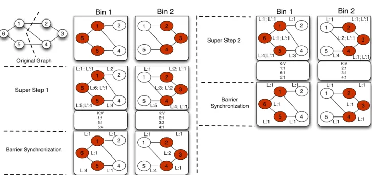
Figure 8 shows an example bitmap setting for the sub-graphs extracted in Figure 3. In Bin 2, subsub-graphs 2 and 3 share nodes 6 and 7 which have both the bits in the vector bitmap set to 1 indicating that they belong to both the
sub-Bin 2: SG-2, SG-3 Bin 1: SG-1,SG-4 2 5 10 4 8 10 6 11 7 2 1 0 1 0 1 0 0 1 0 1 1 1 1 0 1 1 1 1 1 0
Fig. 8 Bitmap based parallel execution
0 500 1000 1500 2000 2500 3000 3500 4000 4500 0 50 100 150 200 250 24 100 500 1000 2000 5000 7000 10000 20000 30000 108577 Me m or y Fo ot pr in t ( MB ) Ex ec u4 on Tim e (Se cs) Batch Size
With Batching No Batching Bitmap Mem Reqd
LCC: For 108577 Subgraphs (a) 0 2000 4000 6000 8000 10000 12000 14000 0 200 400 600 800 1000 1200 1400 24 100 500 1000 2000 5000 7000 10000 20000 30000 325729 Me m or y Fo ot pr in t ( MB ) Ex ec u4 on Tim e (Se cs) Batch Size
No Batching With Batching Bitmap Mem Reqd
LCC: For 325729 Subgraphs
(b)
Fig. 9 Effect of batching on execution time and memory footprints on
two different graph datasets.
graphs. All other nodes in the bins have only one of their bits set, indicating appropriate subgraph membership. Batching Bitmap Mode. As the system scales to a very large number of subgraphs per reducer, the memory con-sumed by the bitmaps can grow rapidly. At the same time, the maximum parallelism that can be achieved is constrained by the hardware configuration, and it is likely that only a small number of subgraphs can actually be processed in par-allel. The batching bitmap mode exploits this by limiting up front the number of subgraphs that may be processed in par-allel. Specifically, we batch the subgraphs into batches of a fixed size (calledbatch-size), and process the subgraphs one batch at a time. A bitmap of lengthbatch-size is sufficient now to indicate to which subgraphs in the batch a vertex or a node contributes. After a batch is finished, the bitmaps are re-initialized and the next batch commences.
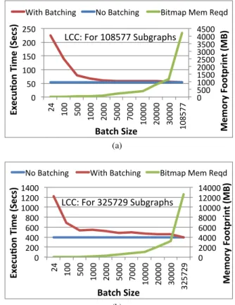
The key question is how to set the batch size. A small batch size may impact the parallelism and may lead to an
increased total execution time. A small batch size is also susceptible to the straggler effect, where the entire batch completion is held up for one or a few subgraphs (leading to wasted resources and low utilization). A very large batch size, on the other hand, can lead to high memory overheads for negligible reductions in total execution time.
Figures 9(a) and 9(b) show the results of a set of exper-iments that we ran to understand the effect of batch size on total execution time and the amount of memory consumed. As we can see, a small batch size indeed leads to underuti-lization of the available parallelism and consequently higher execution times. However, we also observe that beyond a certain value, increasing the batch size further did not lead to significant reduction in the execution time. We do a small penalty for batching that can be attributed to the overhead of reinitializing bitmaps across batched execution and to minor straggler effects. However, there is a wide range of param-eter values where the execution time penalty is acceptable, and the total memory consumed by the bitmaps is low. Based on our evaluation, we set the batch size to be 3000 for most of our experiments; a lower number should be used if the hardware parallelism is lower (these experiments were done on a 24-core machine), and a higher number is warranted for machines with more cores.
Single-Bit Mode. To further reduce the memory overhead associated with bit vectors, we provide a single bit execu-tion mode wherein each node and edge is associated with a single bit which is set if the node participates in the current subgraph computation. The subgraphs are processed in a se-rial order, one at a time, with the bits re-initialized after each computation is finished. This mode is supported to cater to distributed computation on low end commodity machines, but it is not expected to scale to large graphs.
6.2 Bitmap Implementation
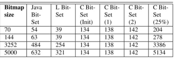
Given the central role played by bitmaps in our execution en-gine, we carefully analyzed and compared different bitmap implementations that are available for use in NSCALE. Java BitSet.Java provides a standard BitSet class that im-plements a vector of bits that grows as needed. The Java Bit-Set class provides generic functionality implementing ad-ditional interfaces and maintains some adad-ditional state to support this functionality. As a consequence, as the bitmap size grows, the Java BitSet object can take up a significant amount of memory, resulting in a relatively high memory overhead.
LBitSet.To reduce the memory overhead of the Java BitSet class, we implemented the LBitSet class as a bare bones im-plementation; LBitSet uses an array of Java primitive type ’long’ (64 bits). Depending on the bitmap size, an appropri-ate size of the array is chosen. To set a bit, the long array
Bitmap size Java Bit-Set L Bit-Set C Bit-Set (Init) C Bit-Set (1) C Bit-Set (2) C Bit-Set (25%) 70 54 39 134 138 142 204 144 63 39 134 138 142 278 3252 484 254 134 138 142 3386 5000 632 321 134 138 142 5134
Table 2 Memory footprints in Bytes for different bitmap constructions
and bitmap sizes in bits. For CBitSet, the table shows the initial mem-ory footprint and how it increases when 1 bit is set, 2 bits are set and 25% bits are set (#bits set indicate the #subgraphs the vertex is part of).
is considered as a contiguous set of bits and the appropriate bit position is set to 1 using binary bit operations. To unset a bit the corresponding bit index position is set to 0. LBitSet incurs less memory overhead than native Java BitSet, which also uses an array of longs underneath, for the reasons de-scribed above.
CBitSet.The CBitSet Java class has been implemented us-ing hash buckets. Each bit index in the bitmap hashes (maps) to a unique bucket which contains all the bitmap indexes that are set to 1. To set a bit, the bit index is added to the corresponding hash bucket. To unset a bit, the bit index is removed from the corresponding hash bucket if it is present. This bitmap construction works on the lines of set associa-tion, wherein we can hash onto the set and do a linear search within it, thereby avoiding allocation of space of all bits ex-plicitly.
We conducted a micro-benchmark comparing these bitmap implementations to get an estimate of the memory over-head for each bitmap, using a memory mapping utility. Ta-ble 2 gives an estimate of the memory requirements per node for each of these bitmaps. Memory footprints for CBitSet shown in the table include a column for the initial allot-ment when the bitmaps are initialized. At run time, when bits are set, this would increase (by about 4 bytes per bit set). The table shows the increase in CBitSet memory as 1, 2, and 25% bits are set. The number of bits set in each bitmap is indicative of the overlap among them. As we can see, CBitSet would have a lesser memory footprint if the overlap is less. In other cases LBitSet has the least memory footprint. A more detailed performance evaluation of the dif-ferent bitmap implementations can be found in Section 8.3.
6.3 Support for Iterative computation.
NSCALEcan naturally handle iterative tasks as well where information must be exchanged across subgraphs between iterations. Below we briefly sketch a description of NSCALE’s iterative execution model.
Execution model.NSCALEuses the Bulk Synchronous Pro-tocol (BSP), used by Pregel, Giraph, GraphX, and several other distributed graph processing systems. The analysis task