DigitalCommons@University of Nebraska - Lincoln
DigitalCommons@University of Nebraska - Lincoln
Finance Department Faculty Publications
Finance Department
4-2008
Securitization of Catastrophe Mortality Risks
Securitization of Catastrophe Mortality Risks
Yijia Lin
University of Nebraska-Lincoln, [email protected]
Samuel H. Cox
University of Manitoba, [email protected]
Follow this and additional works at: https://digitalcommons.unl.edu/financefacpub Part of the Finance and Financial Management Commons
Lin, Yijia and Cox, Samuel H., "Securitization of Catastrophe Mortality Risks" (2008). Finance Department Faculty Publications. 12.
https://digitalcommons.unl.edu/financefacpub/12
This Article is brought to you for free and open access by the Finance Department at DigitalCommons@University of Nebraska - Lincoln. It has been accepted for inclusion in Finance Department Faculty Publications by an authorized administrator of DigitalCommons@University of Nebraska - Lincoln.
1. Introduction
Securities with mortality risk as a component have been around a long time. These securities arise as securitization of portfolios of life insurance or annuity policies. The risks underlying a life insurance or annuity portfolio include in-terest rate risk and policyholder lapse risk, as well as mor-tality or longevity risk. In these transactions, the posi-tive future net cash flow from the policies is dedicated to pay the bondholders. Therefore, they are similar to asset securitization. Cowley and Cummins (2005) surveys recent life insurance securitization transactions, including these asset-type securities.
However, securitization of pure mortality or longevity risk is a recent and potentially important innovation in fi-nancial markets. Pure mortality or longevity securitization is more like property-linked catastrophe bonds than the com-mon asset-type life insurance securitizations. This is be-cause, like that of a property-linked catastrophe bond based on earthquake or hurricane losses, the payment of a mortal-ity securmortal-ity is only subject to a well-defined risk. In the case of a mortality bond, the event might be a sudden spike in death rates, which may be caused by a flu epidemic.
Catastrophes impose a big potential problem for a life
insurer’s solvency since fatalities from natural and man-made disasters may be tremendous. For example, the earth-quake and tsunami in southern Asia and eastern Africa in December 2004 killed 182,340 people and made 129,897 missing (Guy Carpenter, 2005). Although most of the vic-tims did not purchase life insurance, the life insurance in-dustry may not have enough capacity to cover this type of catastrophe losses if such an event were to occur in a more economically developed region where most of people buy life insurance. Cummins and Doherty (1997) noted that “a closer look at the industry reveals that the capacity to bear a large catastrophic loss is actually much more limited than the aggregate statistics would suggest.”
Longevity risk is the other side of mortality risk. Al-though mortality improves over time, future rates of im-provement are uncertain. At the same time we are seeing, especially in the US, a trend to shift longevity risk to indi-viduals. In the US, defined benefit pension plans are con-verting to defined contribution plans. Proposed Social Se-curity reforms further shift mortality risk to individuals. Thus, there should be an increased demand for individual annuities. As the demand for annuities increases, the annu-ity insurers’ need for risk management of potential mortal-ity improvements will increase.
Published in Insurance: Mathematics and Economics42:2 (April 2008), pp. 628-637; doi 10.1016/j.insmatheco.2007.06.005 Copyright © 2007 Elsevier Ltd. Used by permission. http://www.elsevier.com/locate/ime
Submitted March 4, 2006; revised June 13, 2007; accepted June 14, 2007; published online July 18, 2007.1
Securitization of Catastrophe Mortality Risks
Yijia Lin
Department of Finance, University of Nebraska - Lincoln, P.O. Box 880488, Lincoln, NE 68588, USA (Corresponding author: tel 402 472-0093, email [email protected] )
Samuel H. Cox
Dr. L. A. H. Warren Chair Professor of Actuarial Science, University of Manitoba, Winnipeg, Manitoba R3T 5V4, Canada (tel 204 474-7426)
Abstract
Securitization with payments linked to explicit mortality events provides a new investment opportunity to investors and financial institutions. Moreover, mortality-linked securities provide an alternative risk management tool for insurers. As a step toward un-derstanding these securities, we develop an asset pricing model for mortality-based securities in an incomplete market framework with jump processes. Our model nicely explains opposite market outcomes of two existing pure mortality securities.
628
1 This paper was presented at the 2005 World Risk and Insurance Economics Congress Meeting, the 2006 Asia-Pacific Risk and Insurance
Associa-tion Annual Meeting, the 2006 American Risk and Insurance AssociaAssocia-tion Annual Meeting, and the 2006 Financial Management AssociaAssocia-tion An-nual Meeting. It won the 2006 Asia-Pacific Risk and Insurance Association Harold D. Skipper Best Paper Award. We appreciate helpful comments from Patrick Brockett, Richard MacMinn, Naresh Bansai, and other participants at these meetings. We are especially grateful to detailed and in-sightful comments from an anonymous referee.
As a new risk management tool, mortality securiti-zation enhances the capacity of the life insurance indus-try by transferring its catastrophic losses to financial markets. Jaffee and Russell (1997) and Froot (2001) argue that insurance securitization offers a potentially more effi-cient mechanism for financing catastrophe losses than con-ventional insurance and reinsurance. Securitization brings more capital and provides innovative contracting features for the life insurance industry to bear potential mortal-ity shocks, thus avoiding the market disruptions caused by prohibitive reinsurance prices and availability cycles. Moreover, because mortality securities may be uncorre-lated with financial markets, they provide a valuable new source of diversification for market participants (Cox et al., 2000; Litzenberger et al., 1996; Canter et al., 1997). Finally, Cowley and Cummins (2005) categorizes securitization as arbitrage opportunities or new classes of risk that enhance market efficiency.
The first pure death-risk linked deal was the three-year Swiss Re bond issued in December 2003 (Swiss Re, 2003; MorganStanley, 2003; The Actuary, 2004). Almost one year later, the European Investment Bank (EIB) issued the first pure longevity-risk linked deal — a 25-year 540 mil-lion pound (775 milmil-lion euro) bond as part of a product de-signed by BNP Paribas aimed at protecting UK pension schemes against longevity risk.2 In 2004, the Swiss Re Com-pany issued two more mortality bonds. The Swiss Re deal is a hedge against catastrophic loss of insured lives that might result from natural or man-made disasters in the US or Europe. The EIB deal is a security to transfer the other tail of mortality risk, longevity risk, to bondholders.
Interestingly, the market outcomes of the first two mor-tality bonds are opposite. According to MorganStanley, “the appetite for this security [the Swiss Re bonds] from inves-tors was strong.” This is the same reaction invesinves-tors have had to the so-called “catastrophe bonds” based on portfo-lios of property insurance. The strong appetite for mortality securities may indicate a growing potential market for mor-tality securities (Lin and Cox, 2005). On the other hand, the EIB bond has not sold very well at all.
It is important to understand why investors viewed the Swiss Re bond price favorably, yet do not buy the EIB bond. To evaluate these two bonds, we need a model that can capture and price mortality risks. We notice there are only a few preliminary papers in this area. Developing as-set pricing theory in this area is important since it will help market participants better understand this new financial instruments. Most of the existing mortality securitization pricing papers have two major shortcomings. First, they ig-nore mortality jumps (Lee and Carter, 1992; Lee, 2000; Ren-shaw et al., 1996; Sithole et al., 2000; Milevsky and Promis-low, 2001; Olivieri and Pitacco, 2002; Dahl, 2003; Cairns et al., 2004) to model death-linked securities. Mortality jumps should not be ignored in mortality securitization modeling especially on the death side since the rationale behind
sell-ing or buysell-ing mortality securities is to hedge or take catas-trophe risks.3 Second, they use the complete market pric-ing methodology. At this point, it looks like mortality risk bonds cannot be replicated with traded securities. There-fore, we propose to price mortality bonds with the Wang transform, a technique that allows pricing new securities relative to securities whose prices are known.
The Wang transform is a market-based equilibrium pric-ing method that unifies the finance and insurance pricpric-ing theories (Wang, 2002). Wang (2004) recently applied the Wang transform to the property-linked catastrophe securi-ties. Apparently our application of the Wang transform to mortality bonds is new. We also use a jump model for mor-tality dynamics to price the Swiss Re bond linked to cat-astrophic death risk. Moreover, we improve the existing literature (Lin and Cox, 2005) on pricing longevity risk by taking into account parameter uncertainty. Our models en-able investors to better understand why the Swiss Re deal is an attractive investment despite the uncertainty associ-ated with catastrophic mortality risks while the EIB bond has not sold very well.
The paper proceeds as follows. Section 2 describes the current mortality securitization market and the designs of the first two mortality bonds — the Swiss Re and EIB bonds. The two-factor Wang transform as an incomplete market pricing method is introduced in Section 3. In Sec-tion 4, we propose a mortality stochastic model with jumps to price the Swiss Re bond linked to catastrophic death risk. We show that the jump process plays an important role in mortality securitization modeling. We also improve the model in Lin and Cox (2005) to price longevity risk imbed-ded in the EIB bond by taking into account parameter un-certainty. Our models nicely explain the opposite market outcomes of these two bonds. Section 5 is a final discussion and conclusion.
2. Mortality securitization markets
Lane and Beckwith (2005) describe recent activity in the insurance securitization market. In the past ten years, in-surance and capital market are converging. Capital mar-ket investors search for uncorrelated risk for diversification and the risk-adjusted excess return “”. Insurance-linked securities have low or no correlation with financial mar-kets, providing diversification. Moreover, the existing in-surance-linked securities provide high risk-adjusted excess return. They attract more and more investors. For exam-ple, hedge funds increased their investment in insurance-linked securities. At the same time, insurers are looking for new sources of risk financing in the capital markets. Before 1999, there were only seven insurance-linked securities in a total dollar amount of only $886.1 million. However, in-surance securitization increased in both dollar amounts and the number of issues especially in the last two years. There are 27 and 21 transactions in 2004 and 2005 with
dol-2 From http://www.IPE.com on November 8, 2004.
3 Catastrophic death events like earthquakes or epidemics, in most cases, occur unanticipatedly and only last a short time period (e.g. one year).
On the other hand, longevity risk dynamics are a more gradual process and span a long time period. Therefore, modeling mortality jumps seems more important for securities linked to death risk.
630 lin & coxin Insurance: MatheMatIcsand econoMIcs 42 (2008) lar amounts $1894.60 million and $1803.30 million
respec-tively (Lane and Beckwith, 2005). The insurance securitiza-tion includes three “pure” mortality bonds in the US and one in the Europe since December 2003. The first two pub-licly known pure mortality securities are the Swiss Re bond issued in December 2003 (Swiss Re, 2003; MorganStanley, 2003; The Actuary, 2004) and the European Investment Bank (EIB) longevity risk bond issued in November 2004. 2.1. Design of the Swiss Re bond
The financial capacity of the life insurance industry to pay catastrophic death losses from hurricanes, epidem-ics, earthquakes, and other natural or man-made disasters is limited. To expand its capacity to pay catastrophic mor-tality losses, the Swiss Reinsurance Company, the world’s second-largest reinsurance company, obtained $400 million in coverage from institutional investors after its first pure mortality security. Swiss Re issued the bond in late Decem-ber 2003. It matured on January 1, 2007. So it is a three-year deal. The principal is exposed to mortality risk. The mor-tality risk is defined in terms of an index qt in year t based on the weighted average annual population death rates in the US, UK, France, Italy and Switzerland. If the index qt (t = 2004, 2005, or 2006) exceeds 130% of the actual 2002 level, q0, then the investors will have a reduced principal pay-ment. The following equation describes the principal loss percentage, Xt, in year t:
0 if qt ≤ 1.3q0
losst =
{
1 – (1.5q0 – qt)/0.2q0 if 1.3q0 < qt ≤ 1.5q0 (1) 1 if qt > 1.5q0where qt = weighted average population mortality in the US, UK, France, Italy, and Switzerland in year t. q0 = Year 2002 level. Therefore, the payment at maturity is equal to Payment at Maturity = 400,000,000 100% – t∑= 2006 2004losst if t∑= 2006 2004losst < 100% ×
{
0 if t∑= 2006 2004losst ≥ 100% (2) Since the probability of having two mortality catastrophes in a row is negligible, Equation (2) approximates toPayment at Maturity ≈ 400,000,000 1 if q ≤ 1.3q0 ×
{
(1.5q0 – q)/0.2q0 if 1.3q0 < q ≤ 1.5q00 if q > 1.5q0 (3) where q = max(q2004, q2005, q2006).
2.2. Design of the EIB longevity bond
About one year after the Swiss Re bond issue, in No-vember 2004, the EIB issued a longevity bond to provide a solution for financial institutions looking for instruments to hedge their long-term systematic longevity risks. This bond
is the result of the co-operation between the BNP Paribas as structurer/manager, the European Investment Bank (EIB) as issuer and the PartnerRe as the provider of analysis, ex-pertise and risk-taking capacity. The total value of the is-sue was £540 million (775 million euro). It was primarily intended for purchase by UK pension plans (Cairns et al., 2005). The term of the EIB bond is 25 years. Potential buy-ers of the EIB bond are pension plans, as the bond transfers longevity risks to investors.
Here is how the EIB bond works: The bond’s cash flows will be based on the actual longevity experience of the Eng-lish and Welsh male population aged 65 years old, as pub-lished annually by the Office for National Statistics. The future cash flows of the bond will be equal to the amount of a fixed annuity, £50 million, multiplied by the percent-age of the reference population still alive at each anniver-sary. The cash flows, therefore, decline over time. Figure 1 shows projected coupons (payable annually) based on the projected survival rates produced by the UK Government Actuary’s Department (GAD).
3. Incomplete market pricing method—the two-factor Wang transform
Pricing derivative securities in complete markets in-volves replicating portfolios. For example, if we have a traded bond and stock index, then options on the stock index can be replicated by holding bonds and the index, which are priced. The analogy for the Swiss Re bond does not work. The bond is a mortality derivative, but we have no efficiently traded mortality index with which to create a replicating hedge. Situations like this are called incomplete markets. Pricing in this situation must rely on some other assumption — there is no traded underlying security.
Wang (1996, 2000, 2001, 2002) develop a method of pric-ing risks that unifies financial and insurance pricpric-ing the-ories. We can apply it to the incomplete market situation. Wang’s method transforms the underlying distribution in such a way that prices are discounted expected values. The transform has many desirable properties. It has a clear economic interpretation since it can recover the capital as-set pricing model (CAPM) for underlying asas-sets and the Black–Scholes formula for options.
3.1. The Wang transform
Consider a random payment X paid at time T. If the cu-mulative density function is F(x), then a transform is called Figure 1. Projected coupons of the EIB longevity bond. The vertical axis shows projected cash flows (millions of pounds) and time is on the horizontal axis.
the Wang transform if the “distorted” or transformed dis-tribution F*(x) is determined by the market price of risk λ according to the equation
F*X = Φ[Φ–1(F
X(x)) + λ], (4) where Φ(x) is the standard normal cdf. F*X(x) in Equation (4) is called the one-factor Wang transform of FX(x). In the insurance world, the market price of risk λ in the Wang transform reflects the level of market systematic risk and firm-specific unhedgeable risk. The idea is that, after trans-formation, the fair price of X should be the discounted ex-pected value using the transformed distribution.
The one-factor Wang transform assumes that the true distribution is known. However, in reality, we can at best estimate the parameters of a probability density function by a sample out of the population. To account for this, Wang (2002) suggests the two-factor transform:
F*X(x) = Q[Φ–1(F
X(x)) + λ], (5) where Q is the t-distribution. As in the one-factor model in Equation (4), the discounted expected value under the transformed distribution F*X(x) in Equation (5) is the price of X.
We can determine λ from the retail market for life in-surance or annuities by Equation (5) so that at time 0 the price of a life insurance or annuity contract with payment X at time T is its discounted expected value using the trans-formed distribution. Therefore the formula for the price is
vTE*(X) = vT ⌡⌠xdF*(x) (6) where vT is the discount factor determined by the market for risk-free bonds at time 0. Thus, for an insurer’s given li-ability X with cumulative density function F(x), the Wang transform will produce a “risk-adjusted” density function F*(x). The discounted expected value under F*(x), denoted by vTE*[X], is the price of X at time 0. Wang (1996, 2000, 2001, 2002) describe the utility of this approach, showing that it generalizes well-known techniques in finance and insurance.
Suppose an insurer transfers its longevity risk to the fi-nancial market by issuing a longevity bond. We can de-rive the market price of risk λ based on the annuity retail market, then use the same λ to price the longevity bond. If there are no transaction costs between the insurance mar-ket and the financial marmar-ket and annuities were actually traded, our method guarantees no arbitrage opportunity between these two markets. There is another way to view this. Insurers price these life and annuity obligations using a distribution (usually privately held) of future life time. We get to observe the insurers’ prices and use an industry market distribution (known to all) F(x). From the prices, we are able to derive the market price of risk λ so that the ob-served retail life insurance or annuity prices are discounted expected values using F*(x). Then we transfer the same λ to the bond market and use the F*(x) to price mortality-linked bonds. As a result, the insurer uses the same mortality as-sumptions to price the mortality bond as it uses in pricing retail life insurance or annuities.
3.2. Why transform?
According to the classical CAPM with the complete market assumption, the risk premium of an asset should be zero if its payoffs are uncorrelated with those of the ket portfolio. The insurance market is an incomplete mar-ket which violates the complete marmar-ket assumption in the CAPM. Therefore, the CAPM cannot explain the pos-itive and very high risk premium of insurance-linked se-curities whose risk has no or low correlation with that of financial markets. By maximizing the ex post value of the firm, Froot and O’Connel (1997), Froot and Stein (1998) and Froot (2007) suggest that the high risk premium of in-surance-linked securities or reinsurance reflects the risk aversion of insurers or investors when they face unhedge-able insurance risks. Risk aversion of the insurers may arise from the fact that the true economic capital requirements of insurance/reinsurance business are not straightforward and potential financial distress costs are very high (Minton et al., 2004). On the other hand, risk aversion of investors may arise from their loss aversion and/or default risk, po-tential moral hazard behavior and basis risk of the insur-ance-linked security issuing firm (Doherty, 1997). Consis-tent with the theories of Froot and O’Connel (1997), Froot (2007) and Doherty (1997), the transformed distribution in the Wang transform reflects the risk aversion of insurers and investors to unhedgeable risks. In Section 4, we show that the transformed mortality distribution has a longer tail (i.e. higher probability of having catastrophes) than the physical distribution. Evidently insurers and investors are risk averse to catastrophic mortality events.
4. Mortality securitization modeling
Mortality securitization modeling depends on two indis-pensable parts: (1) the mortality forecasting theory and (2) the incomplete market pricing theory. First, the principal or coupons of a mortality security are determined by future mortality levels. For example, the principal of the Swiss Re bond will be reduced if the future population mortality index increases by more than 30% relative to the 2002 level. There-fore we need a model to describe future mortality stochas-tic processes. Second, the insurance market is an incomplete market. If we transfer insurance risks to the financial market by selling insurance-linked securities, we should use an in-complete market pricing method to price these securities. 4.1. Existing mortality securitization modeling
4.1.1. Existing mortality forecasting literature
Mortality securitization modeling is based on the anal-ysis of future mortality dynamic processes. The mortality dynamics include “normal” deviations from the trend and “unanticipated” mortality shocks. Since the rationale be-hind selling or buying mortality securities is to hedge or take catastrophe mortality risks, a good mortality stochas-tic model should take into account mortality jumps—which might be caused by epidemics, wars, or natural catastro-phes such as tsunamis.
Most of the existing mortality forecasting papers do not explicitly model mortality jumps when they describe
fu-632 lin & coxin Insurance: MatheMatIcsand econoMIcs 42 (2008) ture mortality stochastic processes. Dahl (2003) and
Mi-levsky and Promislow (2001) model the force of mortality as an Itô-type stochastic process in continuous time with continuous sample paths. Cairns et al. (2004) use a more so-phisticated approach, but still it is a continuous time model with continuous sample paths. Econometric methods, like Renshaw’s method (Renshaw et al., 1996; Sithole et al., 2000) and the Lee–Carter model (Lee and Carter, 1992; Lee, 2000), do not explicitly take into account mortality jumps either. We propose a model with a jump, or regime switch, to indicate the presence of an event such as a flu epidemic. Our model can be much more simple than those cited here, since we need a model of the population mortality, a single number each period, rather than an entire mortality table in each period. Therefore we choose a simple model, a two-state regime-switching log-normal model. We estimate the model and illustrate it by pricing a death-linked security, the Swiss Re bond.
There are only a few papers that show how to price mor-tality-linked securities. Cairns et al. (2004) price mortal-ity securities in the context of a complete market measure, providing a very important advance in modeling, but we do not have enough data to apply it. And we are not sure how one would estimate the model. On the other hand, we use the Wang transform, which does not require a com-plete market, only a reference price.
4.2. Our model for Swiss Re bond
The Swiss Re bond links bondholder payoffs to a popu-lation mortality index. This provides transparency, reduc-ing moral hazard, since the population index is a weighted average of government-produced mortality statistics. 4.2.1. Model
Our approach combines a Brownian motion and a dis-crete Markov chain with log-normal jump size distribution with parameters m and s. Most of mortality jumps, e.g. the 1918 flu or 2004 earthquake and tsunami, are one-time events. It is true for the death side in most cases. However, mortality usually improves over a long period. We use an-other method to price the EIB bond which is discussed in Section 4.3. Catastrophes push up the whole population death rate just for that bad year. The mortality curve af-ter the shock is independent of that during the shock. Our model takes this into account.
The discrete Markov chain counts the number of events Nt during years t = 0, 1, 2, … with N0 = 0 and transition
Nt+1 = Nt + 1, with probability p
{
Nt, with probability 1 – p. (7) We describe the US population mortality index ~qt dy-namics at time t as a geometric Brownian motion qt when there are no events:dqt/qt = dt + σdWt . (8) The variable is the instantaneous expected force of the US population mortality index. σ is the instantaneous
volatil-ity of the mortalvolatil-ity index, conditional on no jumps. Wt is a standard Brownian motion with mean 0 and variance t. The equivalent explicit description of the index, assuming no events in (t − h, t), is
qt = qt–he( – σ2/2)h + σ(Wt – Wt–h) . (9) The percentage change in the mortality rate due to a ran-dom jump is denoted by Y − 1. The Markov chain and the jump size Y distributions are independent (and indepen-dent of W). A jump event occurs during the period [t − h, t] with probability p. When a jump occurs, there is a shock ef-fect Yt on qt. We express the mortality index, including the jump, as ~qt= qtYtfor t = 0, h, 2h, 3h, …. Our data consist of annual observations so h = 1.
If there is no jump in [t − h, t], then Yt = 1 and q~t= qt . When there is a jump, we assume that Yt is log-normally distributed with parameters m and s. That is, Yt = em + sUt where the Ut is a standard normal variable. In summary, if the index assuming no event is
qt = q0e( – σ2/2)h + σWt for t ≥ 0,
then the US population mortality index ~qt can be explicitly described as follows: ~qt =
{
qtYt with probability p qt with probability 1 – p (10) for t = h, 2h, 3h, ... where Yh, Y2h,… are either 1 (with probability 1 − p) or in-dependent log-normal variables with parameters m and s.The mortality index ~q
t, independent of previous mortal-ity jumps, will be continuous most of the time with finite jumps of differing signs and amplitudes occurring at dis-crete points of time. Let t denote the events determined by the processes Ws, Ns, and Yt for s ≤ t. We apply Equation (10) to get and expression for the index at the end of the pe-riod [t − h, t] in terms of the index without jumps.
~
qt+h|t = qt exp
[
( – σ2/2)h + σ(Wt+h – Wt)
]
Yt+h. (11) In effect, a jump impulse during [t − h, t] has no effect dur-ing [t, t + h].Now we apply the maximum likelihood method to es-timate the parameters , σ, p, m, and s from the data. The term σ(Wt+h − Wt) describes the continuous part of the un-anticipated “normal” mortality index change and Y − 1 describes the percentage change due to an “abnormal” mortality shock with probability p when Nt+h − Nt = 1. Ap-pendix shows the derivation of our maximum likelihood function from Equation (11).
4.2.2. Data
Our data are obtained from the Vital Statistics of the United States (VSUS).4 The VSUS reports the United States age-adjusted death rates per 100,000 standard million
population (2000 standard) for selected causes of death. Age-adjusted death rates are used to compare relative mor-tality risks across groups and over time; they are the in-dexes rather than the direct measures. We plot our data from 1900 to 1998 in Figure 2.
Figure 2 shows that the mortality stochastic process does not follow a mean-reverting process.5 Moreover, there are several jumps in the US population mortality evolution which should be captured by a good mortality stochastic model. Mortality shocks may cause financial distress or bankruptcy of insurers or pension plans and they are also the risks underlying the mortality securities.
4.2.3. Estimation results
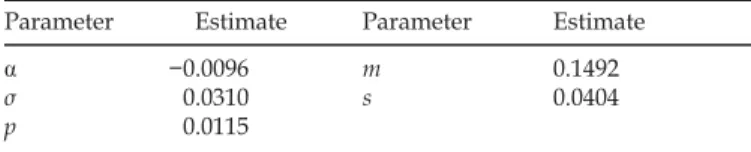
Based on the US population mortality index qt from 1900 to 1998 shown in Figure 2, Table 1 reports our maxi-mum likelihood estimation results. The instantaneous ex-pected force of mortality index is equal to −0.0096. The negative sign of suggests the US population mortality im-proves over time. The instantaneous volatility of the mor-tality index, conditional on no jumps, σ, is equal to 0.0310. The probability of a jump event each year is equal to 1.15%. Our likelihood ratio test rejects the model without jumps at the significance level of 0.1%.
4.2.4. Market price of risk
In this section, we show how to estimate the market price of risk of the Swiss Re bond. First, we simulate Equa-tion (11) with the estimates shown in Table 1 to get cumula-tive probabilities F(q), where q is the maximum of the sim-ulated US population mortality index qt from 2004 to 2006. We run 10,000 simulations.
Second, the physical cumulative probabilities F(q) are transformed by a starting value of the market price of risk
λSR (λSR will be solved later) to get the pricing probabilities F*(q) as shown in Equation (12):
F*(q) = Q[Φ–1F(q) – λ
SR]. (12) Q is the Student’s t-distribution with six degrees of free-dom following Wang (2004). The transformed probabili-ties f*(q) can easily be derived from cumulative probabili-ties F*(q).
Third, after obtaining simulated q values and their trans-formed probabilities f*(q), we calculate the payment at ma-turity following Equation (3). Based on Equations (11) and (12), the par spread of the Swiss Re bond 1.35% (Swiss Re, 2003; MorganStanley, 2003; The Actuary, 2004), the US pop-ulation mortality index from 1900 to 1998 and the US Trea-sury yield rates on December 30, 2003, our estimated mar-ket price of risk λSR of the Swiss Re deal is −1.3603.
In Figure 3, the dashed line denotes the transformed probability density function (PDF) of q with λSR = –1.3603 by using the two-factor Wang transform. It lies on the right of the PDF of simulated US population mortality index “f(q)”. After transforming the data, we put more weight on the right tail. This implies that the market expects a higher probability of having a big loss than the actual probability suggests.
4.2.5. Is the jump process important?
Most of the existing mortality stochastic models do not consider the jump process. In Section 4.2.1, we use Brown-ian motion and the Markov chain to model the dynamics of the US population mortality index. To prove that the jump process is important in the mortality securitization model-ing, we compare the market price of risk without mortality jumps with that with jumps.6
The mortality stochastic model without jumps is shown as follows:
dqt/qt = ndt + σndWt , (13) where n and σn are the expected force and volatility of the Figure 2. 1900–1998 US total population death rate per 100,000 (=
100,000qt where t = 1900, 1901, …, 1998).
Figure 3. Two-factor Wang transformed probability distribution of q = max(q2004, q2005, q2006) with λSR = –1.3603 and six degrees of freedom (shown as a dashed line) and the physical probability distribution of q (shown as a solid line). The horizontal axis is the death rate and the vertical axis stands for the probability.
Table 1. Maximum likelihood parameter estimates based on the US population mortality index 1900–1998
Parameter Estimate Parameter Estimate
−0.0096 m 0.1492
σ 0.0310 s 0.0404
p 0.0115
The model without jumps is rejected at the significance level of 0.1%.
5 But it could be a process that is mean reverting around a trend.
634 lin & coxin Insurance: MatheMatIcsand econoMIcs 42 (2008)
US population mortality index with subscript n indicating no jumps. Based on the same data shown in Section 4.2.2, our maximum likelihood estimate of n is −0.0100 and 0.0388 for σn. Without jumps, our estimated market price of risk for the US-based Swiss Re bond is equal to −1.5545, which is 14% higher than the market price of risk −1.3603 in terms of absolute value when we model the US popu-lation mortality index with jumps. Moreover, we plot the transformed distributions with and without jumps of q in Figure 4. Figure 4 shows that the model without jumps un-derestimates the probability of having a catastrophe death event since the model with jumps has a longer tail. Failing to model jumps leads to a notable deviation from the right market price of risk and the correct transformed distribu-tion. We conclude that the jump process plays an impor-tant role in the mortality securitization modeling.
4.2.6. Is the Swiss Re bond a good deal for investors? Wang (2004) reports that the average market price of risk of property catastrophe bonds is about −0.45. Applying the two-factor Wang transform with λ = −0.45, our calculated par spread for the Swiss Re bond is 0.39%, which is lower than that of the Swiss Re bond, 1.35%. The difference may arise from the fact that we use the US population index as the benchmark while the Swiss Re deal is based on the weighted average of five developed countries. If we use the weighted index, we expect that our calculated par spread will be even lower because of the diversification effect of mortality risks among these five countries. Bantwal and Kunreuther (1999) found the spread of property catastrophe bonds to be too high to be explained by standard financial theory. Here we find the market price of risk of the Swiss Re bond, −1.3603, is even higher than that of the property catastrophe bonds, −0.45 in terms of absolute value. Although the high risk pre-mium of the Swiss Re deal may suggest high transaction costs of the first mortality security, it may also be interpreted as the Swiss Re overcompensating the investors for their tak-ing its mortality risks. So it explains why the “appetite” for the Swiss Re bond was strong.
Why did the Swiss Re company pay such a high risk premium to the investors? The Swiss Re Company’s life reinsurance business accounted for 43% of its group reve-nues in 2002, up from 38% in 2001 (MorganStanley, 2003). Although capital is crucial for a firm to absorb mortality shocks, the true economic capital requirements of life re-insurance business is not straightforward. Moreover, the costs of potential financial distress are high. Minton et al. (2004) conclude that securitization of financial institutions is a contracting innovation aimed at lowering financial dis-tress costs. Therefore, MorganStanley (2003) concludes that Swiss Re must be taking a view that the cost of capital that is relieved via this transaction exceeds the effective net cost of servicing the bond. Moreover, insurance companies pay a high risk premium to develop the mortality securitization market. If catastrophes deplete the traditional reinsurance risk-taking capacity, the insurers can turn to the mortality security market for protection. In all, the Swiss Re mortal-ity bond is a good deal to the investors.
4.3. Our model for the EIB bond
Compared with mortality deterioration caused by catas-trophes like epidemics or earthquakes, mortality improve-ment spans a much longer period. Therefore, we adopt Lin and Cox (2005)’s method to price a longevity bond. Two differences of our method from Lin and Cox (2005) are as follows. First, we use the two-factor Wang transform to ac-count for parameter uncertainty while Lin and Cox (2005) use one-factor model; second, we use the EIB bond price to derive the market price of risk while Lin and Cox (2005) use the US single premium immediate annuity (SPIA) mar-ket quotes.
4.3.1. Our model
We show how to estimate the market price of risk of a longevity bond based on the two-factor Wang transform. We defined our transformed distribution F* for the EIB bond in year t as
F*(tq65) = tq*65 = Q[Φ–1(
tq65) – λEIB] (14) where tq65 is the probability that a person aged 65 dies be-fore age 65 + t and t = 1, 2, …, 25. To calculate the values of tq65 for the English and Welsh male population aged 65, we use the realized mortality rates of English and Welsh males aged 65 and over in 2003. Q is the Student’s t-distribution with six degrees of freedom following Wang (2004). The in-terest rates are the gilt STRIPS on November 18, 2004.
The total value of the EIB bond was £540 million. Its 25-year bond annual payout is equal to a fixed annuity, £50 million, multiplied by the percentage of the reference pop-ulation still alive at each anniversary. Assuming the ex-pense factor 6%, we solve the market price of risk λEIB for the English and Welsh male by the following equation:
540,000,000 × (1 – 0.06) = 50,000,000 a*65:25|― , where a*65:―
25|is the present value of a life annuity of 1 per year, payable in instalments at the end of each year while the annuitant survives for 25 years. The mortality rates in Figure 4. Two-factor Wang transformed probability distribution of
q=max(q2004,q2005,q2006) with λSR = –1.3603 and six degrees of freedom
(shown as a dashed line) in the jump model and that with λSR = –1.5545 and six degrees of freedom (shown as a dotted line) in the model with-out jumps. The x-axis is the death rate and the y-axis stands for the probability.
a*65:―
25|are the distorted mortality rates based on Equation (14).
4.3.2. Market price of risk
Our calculated market price of risk for the EIB bond λEIB is equal to 0.2408. It is not surprising that the market price of risk of the EIB bond (0.2408) is lower than that of the Swiss Re bond (−1.3603) in terms of absolute value since longevity risks have much less immediate and dramatic im-pact on annuity business or pension plans (25 years or lon-ger) than catastrophic death risks caused by disasters like flu (less than a year) on the life insurance business. The in-teresting question here is whether the market price of risk of the EIB bond, λEIB = 0.2408, is too high for the potential bond buyers—the UK pension plans.
Let us compare the market price of risk of the EIB bond λEIB = 0.2408 with that of private annuities. Based on the same idea in Equation (14), our calculated market price of risk of the average SPIA for the US male annuitants aged 65 is only 0.1524.7 The market price of risk reflects the costs of adverse selection. Adverse selection is the tendency of persons with a higher-than-average chance of loss to seek insurance at standard rates, resulting in higher-than-ex-pected loss levels (Rejda, 2005). For example, healthy peo-ple purchase more annuities while those in poorer health buy more life insurance. Prior literature concludes that pen-sion plans have much less adverse selection problem than commercial annuity insurers because both healthy and less healthy employees participate in pension plans. Therefore the longevity risk for a pension plan should be lower than that for a commercial annuity insurer. Since mortality ex-periences of US population and English and Welsh pop-ulation are similar, theoretically, the market price of risk for the EIB bond should be lower than that for the annuity business, 0.1524. However, this is not true for the EIB bond. Therefore, it explains why the UK pension plans, the po-tential buyers of the EIB bond, are not willing to buy the EIB bond since they can get the cheaper protection from the an-nuity or reinsurance markets.
5. Discussion and conclusions
We are learning every day how important mortality forecasts are in the management of life insurers and private pension plans. Securitization and development of mortal-ity bonds can be an important part of capital market solu-tion to these problems. Before the Swiss Re bond was is-sued at the end of 2003, life insurance securitization was not designed to manage mortality risk; rather they are ex-actly like asset securitization. In these cases, the insurers convert future life insurance profits into cash to increase li-quidity rather than manage mortality risk. The new securi-tization we study in this paper focus on the other side of an insurer’s balance sheet—liabilities on future mortality
pay-ments. The introduction of mortality securities to transfer the insurer’s risks in the liabilities side increases its capac-ity and maintains its competitiveness.
A market for mortality-based securities will develop if the prices and contracting features make the securities attractive to potential buyers and sellers. The Swiss Re bond has sold well but the EIB bond has not. We explain these opposite market outcomes by looking at their risk premiums. To cal-culate the risk premiums we need models, analogous to the term structure on interest rate models. The mortality bond market will be richer in that, in addition to default free zero coupon bonds, it will have bonds which will be redeemed at face value only if a specified number of lives survives or dies to the maturity date. We find only a few preliminary papers on this topic. Development of the theory in this direction is important as an extension of traditional bond market models and it would be very useful in explaining mortality market risk to potential market participants.
Our model shows that the Swiss Re mortality bond of-fers a higher risk premium to investors than the property-linked catastrophe bonds. However, the EIB charges a very high risk premium to take longevity risks in the UK pen-sion plans. Since the price of the EIB bond is not attractive, no UK pension plan has bought this bond until now!
Moreover, the EIB bond provides “ground up” protec-tion, covering the entire annuity payment. But the plan can predict the number of survivors to some extent, especially in the early contract years. The EIB bond price includes coverage the plan does not need (including rates, commis-sions, etc.). A more attractive contract might cover pay-ments to survivors in excess of some strike level. The price would be much lower, as shown in Lin and Cox (2005).
Someone may argue that the index-linked mortality se-curities are subject to unacceptable levels of basis risk. The basis risk is lower for the Swiss Re bond than for the EIB bond. The population index of the Swiss Re bond accounts for basis risk by using different weights in five countries to match Swiss Re’s business. However, the EIB bond does not provide a good hedge for a pension plan: there exists a significant basis risk between the reference population mor-tality and that of an individual pension plan. The EIB deal does not allow pension plans to decide their own mortality references (e.g. by using different weights in the Swiss Re bond) to reduce the basis risk. The basis risk problem fur-ther reduces the attractiveness of the EIB bond.
In summary, we contribute to the mortality securitiza-tion literature by proposing a mortality stochastic model with jumps for death-linked insurance securities and pric-ing the Swiss Re and EIB bonds in an incomplete market framework. Our models nicely explain the opposite market outcomes of these two deals. Finally we comment on the structure and basis risk problem of these two bonds. Again, it shows the attractiveness of the Swiss Re deal but not for the EIB bond.
7 We get the market quotes of the non-qualified SPIA in August 1996 from Kiczek (1996). Kiczek (1996) reports the male and female SPIA monthly
payout rates of 102 companies with the $100,000 lump-sum premium at the issue age 65. We assume that an insurer sells its SPIA at the market av-erage payout rates $764 for male. We also assume an expense factor of 6%. Our US Treasury yield rates on August 15, 1996 are obtained from the Wall Street Journal. Our mortality rates are from the 1996 Male IAM 2000 Basic Mortality Table.
636 lin & coxin Insurance: MatheMatIcsand econoMIcs 42 (2008)
APPENDIX. Maximum likelihood estimation of mortality Stochastic model with jumps
After taking the logarithm of both sides of Equation (11), we obtain
log ~qt+h = log qt + ( – σ2/2)h + σ ΔW
t + log Yt+h (15) where Δ denotes the change over [t, t + h]. Let Zt = Δlog ~qt so that
Zt = Δlog ~qt+h – log ~qt = ( – σ2/2)h + σ ΔW
t + log Yt+h – log Yt
The conditional distribution of Zt, given t, is denoted Zt|t. We have observations of the index ~qt for t = h, 2h, … Kh.
If no mortality jump event occurs during the periods [t − h,
t] and [t, t + h], then Yt = Yt+h = 1 and Zt|tis normally distrib-uted with mean Mnn = ( – σ2/2)h and variance S2
nn = σ2h. If a jump event occurs during the period [t − h, t] but not [t, t + h], then Yt = exp(m + sUt) and Yt+h = 1. In this case, Zt|tis nor-mally distributed with mean Myn = ( – ½ σ2)h – m and vari-ance S2
yn = σ2h + s2. There are two other possibilities: no mor-tality jump during the period [t − h, t] but a mortality jump during [t, t + h]; a mortality jump during the period [t − h, t] and another mortality jump during [t, t + h]. We summarize the conditional means and variances of Zt as follows. Given t, we will know if jumps occurred in [t − h, t] and [t, t + h]. Let nn
denote the event “no jumps occurred”; yn the event “a jump occurred in [t − h, t] but no jump occurred in [t, t + h],” and so on. In summary, the distribution is described as follows:
Jump E[Zt|t] Var[Zt|t] Probability events
nn (−σ2/2)h σ2h (1−p)2
yn (−σ2/2)h−m σ2h+s2 p(1−p)
ny (−σ2/2)h+m σ2h+s2 (1−p)p
yy (−σ2/2)h σ2h+2s2 p2
The probability density function of Zt , fZ(z), can be written in terms of the conditional density of Zt|t, denoted fz(z|t), which has a conditionally normal distribution:
(16) We have a time series of K observations of ~qt, where t = 0, 1, 2, …, K − 1, so the step size is h = 1. We have K − 1 obser-vations zt of Zt = log ~qt+1 – log ~qt. The correlations between the zt’s are zero except when jump events occur. The probabil-ity of having a mortalprobabil-ity catastrophe event is very low. Based on the historical data, the correlation introduced by mortality catastrophes to the likelihood function is only around −0.005. Therefore, we use independence as an approximation and es-timate the parameters p, , σ, m, and s by maximizing the loga-rithm of the likelihood function (17) based on the observations
z1, z2, …, zK−1. The likelihood is
K – 1
L = ∏ fz(zt) (17) t = 1
Taking the logarithm of Equation (17), we get
(18)
References
Bantwal and Kunreuther, 1999 ► V. J. Bantwal and H. C. Kunreuther, 1999. A cat bond premium puzzle. Working paper. Financial Insti-tutions Center of the Wharton School.
Cairns et al., 2005 ► Cairns, A. J. G., Blake, D., Dawson, P., Dowd, K., 2005. Pricing the risk on longevity bonds. Working paper. Heriot-Watt University, Edinburgh, UK.
Cairns et al., 2004 ► Cairns, A. J. G., Blake, D., Dowd, K., 2004. Pric-ing frameworks for securitization of mortality risk. WorkPric-ing pa-per. Heriot-Watt University, Edinburgh, UK.
Canter et al., 1997 ► M. Canter, J. Cole and R. Sandor, Insurance de-rivatives: A new asset class for the capital markets and a new hedging tool for the insurance industry, Journal of Applied Corpo-rate Finance10 (3) (1997), pp. 69–81.
Cox et al., 2000 ► S. H. Cox, H. W. Pedersen and J. R. Fairchild, Eco-nomic aspects of securitization of risk, ASTIN Bulletin30 (1) (2000), pp. 157–193.
Cowley and Cummins, 2005 ► A. Cowley and J. D. Cummins, Securi-tization of life insurance assets, Journal of Risk and Insurance72 (2) (2005), pp. 193–226.
Cummins and Doherty, 1997 ► J. D. Cummins and N. A. Doherty, 1997. Can insurers pay for the ‘big one?’ measuring the capacity of an insurance market to response to catastrophic losses. Working paper. The Wharton School, University of Pennsylvania.
Dahl, 2003 ►M. H. Dahl, 2003. Stochastic mortality in life insurance: Market reserves and mortality-linked insurance contracts. Work-ing paper. University of Copenhagen, Denmark.
Doherty, 1997 ► N. A. Doherty, Financial innovation in the manage-ment of catastrophe risk, Journal of Applied Corporate Finance10 (3) (1997), pp. 84–95.
Froot, 2001 ► K. A. Froot, The market for catastrophe risk: A clini-cal examination, Journal of Financial Economics60 (2–3) (2001), pp. 529–571.
Froot, 2007 ► K. A. Froot, Risk management, capital budgeting, and capital structure policy for insurers and reinsurers, Journal of Risk and Insurance74 (2) (2007), pp. 273–299.
Froot and O’Connel, 1997 ► K. Froot and P. O’Connel, 1997. On the pricing of intermediated risks: Theory and application to catastro-phe reinsurance. Working paper. Harvard Business School, Bos-ton, MA.
Froot and Stein, 1998 ► K. A. Froot and J. C. Stein, Risk management, capital budgeting, and capital structure policy for financial institu-tions: An integrated approach, Journal of Financial Economics47 (1) (1998), pp. 55–82.
Guy Carpenter, 2005 ► Guy Carpenter, 2005. Tsunami: Indian Ocean event and investigation into potential global risks. See the report release in March 2005.
Jaffee and Russell, 1997 ► D. M. Jaffee and T. Russell, Catastrophe in-surance, capital markets, and uninsurable risks, Journal of Risk and Insurance64 (2) (1997), pp. 205–230.
Kiczek, 1996 ► J. A. Kiczek, Single premium immediate annuity pay-outs, Best’s Review (L/H)97 (4) (1996), pp. 57–60.
Lane and Beckwith, 2005 ► M. N. Lane and R. G. Beckwith, 2005, April. The 2005 review of the insurance securitization market. Technical Report. Lane Financial LLC, Wilmette, IL.
Lee, 2000 ► R. D. Lee, The Lee–Carter method of forecasting mortal-ity, with various extensions and applications, North American Ac-tuarial Journal4 (1) (2000), pp. 80–93.
Lee and Carter, 1992 ► R. D. Lee and L. R. Carter, Modelling and fore-casting US mortality, Journal of the American Statistical Association 87 (419) (1992), pp. 659–671.
Lin and Cox, 2005 ► Y. Lin and S. H. Cox, Securitization of mortal-ity risks in life annuities, Journal of Risk and Insurance72 (2) (2005), pp. 227–252.
Litzenberger et al., 1996 ► R. H. Litzenberger, D. R. Beaglehole and C. E. Reynolds, Assessing catastrophe reinsurance linked securi-ties as a new asset class, Journal of Portfolio Management22 (1996), pp. 76–86 (special issue).
Milevsky and Promislow, 2001 ► M. A. Milevsky and S. D. Promis-low, Mortality derivatives and the option to annuitize, Insurance: Mathematics and Economics29 (3) (2001), pp. 299–318.
Minton et al., 2004 ► B. Minton, A. B. Sanders, and P. E. Strahan, 2004. Securitization by banks and finance companies: Efficient financial contracting or regulatory arbitrage? Working Paper no. 2004–25, The Ohio State University.
MorganStanley, 2003 ► MorganStanley, 2003. Swiss Re innovative mortality-based security. See the news release for December 8, 2003.
Olivieri and Pitacco, 2002 ► A. Olivieri and E. Pitacco, 2002. Infer-ence about mortality improvements in life annuity portfolios. In: XXVIIth International Congress of Actuaries.
Rejda, 2005 ► G. E. Rejda, Principles of Risk Management and Insur-ance (ninth ed), Addison-Wesley Publishers, New York (2005). Renshaw et al., 1996 ► A. Renshaw, S. Haberman and P.
Hatzoup-oulos, The modeling of recent mortality trends in United King-dom male assured lives, British Actuarial Journal2 (2) (1996), pp. 449–477.
Sithole et al., 2000 ► T. Z. Sithole, S. Haberman and R. J. Verrall, An investigation into parametric models for mortality projections, with applications to immediate annuitants and life office pension-ers data, Insurance: Mathematics and Economics27 (3) (2000), pp. 285–312.
Swiss Re, 2003 ► Swiss Re, 2003. Swiss Re obtains USD 400 million of extreme mortality risk coverage—its first life securitization. See the news release for December 2003.
The Actuary, 2004 ► The Actuary, 2004. Swiss Re obtains $400 million of mortality risk coverage. The Actuary. January/February, P. 16. Wang, 1996 ► S. S. Wang, Premium calculation by transforming the
layer premium density, ASTIN Bulletin26 (1) (1996), pp. 71–92. Wang, 2000 ► S. S. Wang, A class of distortion operations for
pric-ing financial and insurance risks, Journal of Risk and Insurance67 (1) (2000), pp. 15–36.
Wang, 2001 ► S. S. Wang, A universal framework for pricing financial and insurance risks, XI-th AFIR Proceedings 2001, September 6–7, Toronto, AFIR (2001), pp. 679–703.
Wang, 2002 ► S. S. Wang, A universal framework for pricing financial and insurance risks, ASTIN Bulletin32 (2) (2002), pp. 213–234. Wang, 2004 ► S. S. Wang, Cat bond pricing using probability
trans-forms (Insurance and the State of the Art in Cat Bond Pricing), The Geneva Papers on Risk and Insurance — Issues and Practice (2004), pp. 19–29 (special issue).