Radiation heat transfer in OpenFOAM

(1)

Final Assignment

for the course

«CFD with OpenSource Software»

Radiation heat transfer in

OpenFOAM

Student: Alexey Vdovin,

vdovin@student.chalmers.se

Reviewed by: Andreu Oliver González,

andrewo@student.chalmers.se

(2)

2

1.0 Introduction

Radiation heat transfer processes are extremely important, they are concerned with the exchange of thermal energy. Heat transfer through radiation takes place in form of electromagnetic waves. In contrast to heat transfer by conduction and convection, radiative heat transfer requires no medium. The intermediaries are photons which travel at the speed of light.

The heat transferred into or out of an object by thermal radiation is a function of several components like surface reflectivity, emissivity, surface area, temperature, and geometric orientation with respect to other thermally participating objects. In turn, an object's surface reflectivity and emissivity is a function of its surface conditions (roughness, finish, etc.) and composition.

For a huge amount of different purposes it is important to be able to calculate or simulate radiation heat transfer between bodies. To do it, there are several radiation models of different complexity. In this report one can find the information about radiation heat transfer implementation in the OpenFOAM (Open Field Operation and Manipulation) CFD Toolbox. The version of the software used is 1.6.x. This report will answer some questions about how radiation heat transfer can be added to the case, what different radiation heat transfer models are available, and what their advantages and disadvantages are. In addition a deeper look at one of the models (the P1 model) will be taken.

(4)

4

2.0 Addition of the radiation heat transfer to the solver

Having different solvers like buoyantSimpleFoam that is used for steady-state buoyant, turbulent flow of compressible fluids for ventilation and heat transfer, and buoyantSimpleRadiationFoam that is almost the same solver just with added radiation heat transfer, it becomes possible to find out how to add radiation to existing OpenFOAM solvers. These solvers can be found in the folder

$FOAM_APP/applications/solvers/heatTransfer/.

The only difference in buoyantSimpleRadiationFoam.C compared to buoyantSimpleFoam.C are two following lines:

#include "radiationModel.H" #include "createRadiationModel.H"

that includes header files for radiation to the compilation.

All .h files are the same for both solvers except hEqn.H that is modified by the addition of the term

Sh(thermo) to the energy equation:

fvScalarMatrix hEqn ( fvm::div(phi, h) - fvm::Sp(fvc::div(phi), h) - fvm::laplacian(turbulence->alphaEff(), h) == fvc::div(phi/fvc::interpolate(rho)*fvc::interpolate(p)) - p*fvc::div(phi/fvc::interpolate(rho)) + radiation->Sh(thermo) );

This function will be discussed when it comes to the radiation models discussion. Also there is one extra line added to the hEqn.H file:

radiation->correct();

That is used for recalculating radiation as it will be shown further.

Before compilation of the solver it is also needed to add some lines to the Make/options file:

EXE_INC = \

-I$(LIB_SRC)/thermophysicalModels/radiation/lnInclude \ EXE_LIBS = \

-lradiation \

After this modification is done and the solver is compiled, it is ready to solve tasks that include radiation. The only thing left is to choose the radiation model to be used and to add some extra variables, needed by the chosen model, to the existing code.

(5)

5

3.0 Radiation models in OpenFOAM

There are three radiation models available in OpenFOAM. Those and their abstract class will be discussed in this chapter. It can be found in the folder $FOAM_SRC/thermophysicalModels \ /radiation.

3.1 Abstract class for radiation models

In the file $FOAM_SRC/thermophysicalModels/radiation/radiationModel/radiationModel/ \ /radiationModel.C an abstract class named radiationModel can be found.

The most important here are the member functions Rp(), Ru(), and the one that generates a source term of the enthalpy equation - Sh().

For the Sh() member function it can be found:

volScalarField& h = thermo.h(); const volScalarField cp = thermo.Cp(); const volScalarField T3 = pow3(T_); return ( Ru() - fvm::Sp(4.0*Rp()*T3/cp, h) - Rp()*T3*(T_ - 4.0*h/cp) );

Here one can see that enthalpy h[J/kg], heat capacity at constant pressure for patch Cp[J/kg/K], third power of the temperature T3[K^3] and two member function values are used for calculating Sh().

Those member functions Ru() and Rp() are defined differently in the different radiation models. Ru() represents constant part of the source term component that is added to the enthalpy equation and Rp() represents the source term component that goes with the ܶସ, Here one can see that the

fvm::Sp function is used. It is mostly done to redistribute source terms to make the coefficient matrix more diagonally dominant. In terms of the equation being solved one can write:

ܵℎሺ ሻ = ܴݑሺ ሻ − 4ܴ݌ሺ ሻ ∗ܶ_ܥଷℎ

௉ − ܴ݌ሺ ሻܶ

ସ_{+ 4ܴ݌ሺ ሻ ∗}ܶଷℎ ܥ௉ ܵℎሺ ሻ = ܴݑሺ ሻ − ܴ݌ሺ ሻܶସ

In other words adding and subtracting the term 4ܴ݌ሺ ሻ ∗்య௛

஼ು does not affect the result but this

significantly improves numerical stability.

Also in the abstract class one can find the correct() member function which is the one called in

hEqn.H, discussed before. Here is the code for it:

(6)

6

{ if (!radiation_) { return; }

if (time_.timeIndex() % solverFreq_ == 0) { calculate(); } }.

As it can be seen in the code this function calls the calculate() member function that is different for different radiation models.

The abstract class radiationModel has three sub-classes that implement the member functions differently. These are briefly described in the following sections.

3.2 The NoRadiation model

First of as a fast way of disabling radiation heat transfer in the calculation there is a noRadiation

model that sets member functions Ru() and Rp() equal to zero, so that the additional term for the enthalpy equation Sh() is becoming 0, thereby the original enthalpy equation will be unaffected by radiation.

3.3 The finite volume discrete ordinates model

The fvDOM model is another radiation model implemented in OpenFOAM. In this model the radiative heat transfer equation is solved for a discrete number of finite solid angles ߪ_௦.

Advantages of the the fvDOM model:

• It is a conservative method that leads to a heat balance for a coarse discretization. The accuracy can be increased by using a finer discretization,

• It is the most comprehensive radiation model: Accounts for scattering, semi-transparent media, specular surfaces, and wavelength-dependent transmission using banded-gray option. Limitations of the fvDOM model:

• Solving a problem with a large number of ordinates is CPU-intensive. 3.4 The P1 model

The last model implemented in OpenFOAM for radiation heat transfer is the P1 model. The main assumption of this model is that the directional dependence in the radiative transfer equation is integrated out, resulting in a diffusion equation for incident radiation.

Advantages of the P1 model:

• The radiative heat transfer equation is easy to solve with little CPU demand,

• It includes effects of scattering. Effects of particles, droplets, and soot can be included,

• It works reasonably well for applications where the optical thickness is large, ߬ = ܽ ∗ ܮ > 3, where L = distance between objects (e.g. the model can be used in combustion).

Limitations of the P1 model:

• It assumes that all surfaces are diffuse,

• It may result in loss of accuracy (depending on the complexity of the geometry) if the optical thickness is small,

(7)

7

• It tends to overpredict radiative fluxes from localized heat sources or sinks. 3.5 Radiation constants

There is only one constant defined for all radiation models in OpenFOAM and it can be found in the file $FOAM_SRC/thermophysicalModels/radiation/radiationConstants/radiationConstants.C:

const Foam::dimensionedScalar Foam::radiation::sigmaSB ( Foam::dimensionedConstant ( "sigmaSB", dimensionedScalar ( "sigmaSB", dimensionSet(1, 0, -3, -4, 0, 0, 0), 5.670E-08 ) ) );

This is the Stefan-Boltzmann constant that is a constant of proportionality in the Stefan–Boltzmann law: the total energy radiated per unit surface area of a black body in unit time is proportional to the fourth power of the thermodynamic temperature. The value for it is ߪ_ௌ஻ = 5.670 ∙ 10ି଼ ܹ ݉ൗ _ଶ∙ ܭସ. 3.6 Scatter models

Scattering is a process where some radiation is forced to deviate from its original path as a result of interaction with one or more localized non-uniformities in the medium. If including the effect of scattering, the scatter model should be defined. To find available scatter models one should look at

$FOAM_SRC/thermophysicalModels/radiation/submodels/scatterModel folder. Currently there is only one scatter model available, which is called constantScatter. One can find that there is only one member function: Foam::tmp<Foam::volScalarField> Foam::radiation::constantScatter::sigmaEff() const { return tmp<volScalarField> ( new volScalarField ( IOobject ( "sigma", mesh_.time().timeName(), mesh_, IOobject::NO_READ,

(8)

8 IOobject::NO_WRITE, false ), mesh_, sigma_*(3.0 - C_) ) ); }

So this constantScatter model has an input of two coefficients sigma and C. Sigma in this case is called to be a scattering coefficient. Its value is set in units of 1/length. Along with the absorption coefficient, that will be described further, it describes the change in radiation intensity per unit length along the path through the fluid medium. C is a linear-anisotropic phase function coefficient, by default it is assumed to be 0 and scattering to be isotropic. To model anisotropic scattering the value of the phase function coefficient should be set to a value in the interval between -1 and 1. Minus sign represents backward scattering and positive values correspond to forward scattering.

3.7 Absorption-Emission Models

As radiation models are dealing with absorption and emission effects, coefficients for those should be defined. There are three coefficients that are used in radiation models for that purpose:

ܽ ൣ1 ݉ൗ ൧ − ܾܽݏ݋ݎ݌ݐ݅݋݊ ܿ݋݂݂݁݅ܿ݅݁݊ݐ, ݁ ൣ1 ݉ൗ ൧ − ݁݉݅ݏݏ݅݋݊ ܿ݋݂݂݁݅ܿ݅݁݊ݐ, ܧ ቂܹ ݉ൗ ቃ − ݁݉݅ݏݏ݅݋݊ ܿ݋݊ݐݎܾ݅ݑݐ݅݋݊.ଷ

For calculation of those there are several absorption-emission models available in the OpenFOAM, they can be found in the $FOAM_SRC/thermophysicalModels/radiation/submodels/ \ /absorptionEmissionModel folder. In this tutorial the simplest constantAbsorptionEmission model is going to be used. For this model these three coefficients are defined in the radiation model and they are considered to have a constant value.

3.8 Radiation boundary conditions

For solving the case, boundary conditions for the incident radiation intensity G need to be defined. There are a number of different boundary conditions that can be used; they can be found in the

$FOAM_SRC/thermophysicalModels/radiation/derivedFvPatchFields folder.

Here one can find the MarshakRadiation boundary condition that is going to be used in this tutorial. It uses calculated temperature from the case as a temperature for calculating radiation intensity. Another option that can be found in the folder is MarshakRadiationFixedT. For this boundary condition the radiation temperature should be specified, and then this value is used for calculating G.

(9)

9

4.0 The P1 radiation model files

Having checked $FOAM_SRC/thermophysicalModels/radiation/radiationModel/P1 folder, one can find all files that are related to the P1 radiation model and its implementation in OpenFOAM.

By taking a look at the P1.C file the model behavior can be understood. Firstly, the gamma value is calculated using the absorption coefficient a and the value of sigmaEff that is coming from the scatter model as it was described before.

// Construct diffusion

const volScalarField gamma ( IOobject ( "gammaRad", G_.mesh().time().timeName(), G_.mesh(), IOobject::NO_READ, IOobject::NO_WRITE ), 1.0/(3.0*a_ + sigmaEff) );

In terms of formulas the equation for gamma will be:

݃ܽ݉݉ܽ =_{3ܽ + ݏ݅݃݉ܽܧ݂݂}1

Secondly, the incident radiation intensity G transport equation is solved:

solve ( fvm::laplacian(gamma, G_) - fvm::Sp(a_, G_) == - 4.0*(e_*radiation::sigmaSB*pow4(T_) + E_) ); Or in terms of formulas: ∇ ∙ ݃ܽ݉݉ܽ∇ܩ − ܽܩ = −4ሺ݁ߪௌ஻ܶସ+ ܧሻ

Thirdly, the Ru() and Rp() member function definitions can be found. For Rp() the implementation is:

(10)

10

4.0*absorptionEmission_->eCont()*radiation::sigmaSB

or in terms of equations:

ܴ݌ሺ ሻ = 4݁ߪௌ஻

where ߪ_ௌ஻ is Stefan-Boltzmann constant defined in radiationConstants as described earlier.

For the Ru() function one can find the implementation:

return a*G - 4.0*E;

or in terms of equations:

ܴݑሺ ሻ = ܽܩ − 4ܧ

Finally the additional term for the enthalpy equation Sh() for this model looks like:

ܵℎሺ ሻ = ܴݑሺ ሻ– ܴ݌ሺ ሻܶସ

or

ܵℎሺ ሻ = ܽܩ − 4ሺ݁ߪௌ஻ܶସ+ ܧሻ

In other words this additional term represents the amount of emitted radiation subtracted from the amount of absorbed irradiation.

(11)

11

5.0 Case set up for

hotRadiationRoom

_tutorial

To show how to add radiation heat transfer to the case files, one can look at the two tutorials available in the OpenFOAM, those are hotRoom tutorial, that is made to work with

buoyantSimpleFoam solver, and hotRadiationRoom – the one that works with

buoyantSimpleRadiationFoam. In this chapter a deep look into the hotRadiationRoom case files will be given to show what modifications are needed to include radiation heat transfer to the case.

5.1 Case set up

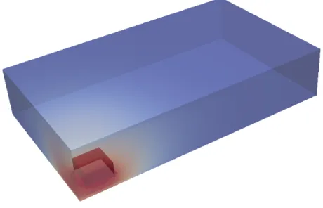
According to /constant/polyMesh/blockMeshDict file there is a room with dimensions of 10x6x2 meters and a box that will represent a heat source 1x1x0.5 meters in dimensions. The temperature of the walls, ceiling and floor is set to 300 K and the temperature of the heater is set to 500 K.

Figure 1. HotRadiationRoom case setup

5.2 Modifications done in tutorial files to make the case work with radiation To make the case work with radiation not only the different solver should be used (buoyantSimpleRadiationFoam instead of buoyantSimpleFoam in this case), but several changes need to be done as well.

Firstly there is a \constant\radiationProperties file, where one can find the following lines:

radiation on; radiationModel P1; … absorptionEmissionModel constantAbsorptionEmission; constantAbsorptionEmissionCoeffs { a a [ 0 -1 0 0 0 0 0 ] 0.5; e e [ 0 -1 0 0 0 0 0 ] 0.5; E E [ 1 -1 -3 0 0 0 0 ] 0;}

(12)

12 scatterModel constantScatter; constantScatterCoeffs { sigma sigma [ 0 -1 0 0 0 0 0 ] 0; C C [ 0 0 0 0 0 0 0 ] 0; }

As it can be seen the radiation model is defined here. It can be set to be “none” to use NoRadiation

model ,“P1” for P1 model or “”fvDOM” for finite volume discrete ordinates model. A few lines after it an absorptionEmissionModel is selected, so the model with constant coefficients for absorption and emission is to be used. The value 0.5 ݉ିଵ is set for both of them. The emission contribution E is set to 0. Also here scatterModel is selected to be constantScatter and coefficients for it are defined.

Another thing to be done is to add boundary conditions for the incident radiation intensity G. So at

/0/ folder file /0/G should be created with the following lines inside:

FoamFile { version 2.0; format ascii; class volScalarField; object G;} // * * * * * * * * * * * * * * * * * * * * * * * * * * * * * * * * * * * * * // dimensions [1 0 -3 0 0 0 0]; internalField uniform 0; boundaryField { floor { type MarshakRadiation; T T; emissivity 1; value uniform 0; } fixedWalls { type MarshakRadiation; T T; emissivity 1; value uniform 0; } ceiling { type MarshakRadiation; T T; emissivity 1; value uniform 0; }

(13)

13 box { type MarshakRadiation; T T; emissivity 1; value uniform 0; } }

As it can be seen, the same conditions are set for all the faces for the room and for the heater.

In addition to everything said before the system/fvSolution file should be modified. Firstly the solver for G variable should be defined:

solvers { … G { solver PCG; preconditioner DIC; tolerance 1e-05; relTol 0.1; } }

and relaxation factor value should be set:

relaxationFactors {

…

G 0.7; }

As all these changes are done the case is ready to work with the radiation heat transfer. So the results for the simulation with and without radiation are compared in the following chapter.

(14)

14

6.0 Results and discussions

Several test cases were run to figure out how the adding of the radiation term affects the simulation. For all of them buoyantSimpleRadiationFoam solver was used. To simulate the case without radiation radiationModel parameter was set to none in the the \constant\radiationProperties

file.

As a good way of presenting result it was decided to use a Y-normal cutting plane that cuts the heater exactly at the middle as it can be seen in the figure 2.

Figure 2. Y-normal cutting plane

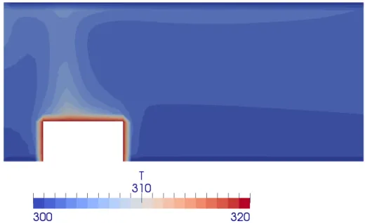
In the figure 3 one can see the temperature distribution at the cutting plane for the case without radiation.

Figure 3. Temperature distribution without radiation heat transfer

Here the hot air moving upwards can be seen, in just few centimeters from the heat source the temperature drops from 500 K almost to the temperature of surrounding air or 300 K. For this reason a scale from 300 K to 320 K degrees was used. Temperatures differ a lot when one uses the model with P1 radiation model added. The result can be seen in the figure 4.

(15)

15

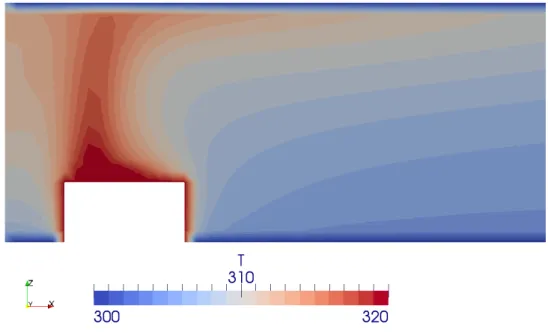
Figure 4. Temperature distribution with radiation heat transfer

The temperature scale for these two pictures is the same so one can see the big difference. As the temperature for the air is increased the air speeds will grow so all case results will be different. For a better understanding of the P1 model that was used, it can be valuable to plot the distribution of incident radiation intensity G. This is done in figure 5.

(16)

16 As one can see, G is inversely proportional to the square of the distance from the heat source. So as it was predictable the air around the box is additionally heated by the radiation heat transfer.

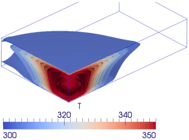
An additional simulation was performed. By setting the gravity constant close to zero in the

constant/g file, the convection effects were decreased. The result of this simulation can be seen below.

Figure 6. Temperature gradient for the case without convection

As predictable, without convection the temperatures are much higher because the heated air is not raising and it is not being replaced by cold one.

7.0 Conclusions

It is obvious that the effect of radiation heat transfer cannot be ignored and it needs to be added to any cases where it can be predicted to have a significant effect. It was shown that the addition of radiation heat transfer to the solver and case files is not a very complicated task. Depending on the complexity of the task being solved and the computational power available different radiation heat transfer models can be selected. One should also keep in mind that there is a need to select a proper scatter model, boundary conditions and absorption-emission model. After all assumptions are done and the values for all needed coefficients are set it is only a matter of time to get the results.

(17)

17

8.0 References

1. Frank P. Incropera, David P.DeWitt, - “Fundamentals of Heat and Mass Transfer”, School of Mechanical Engineering Purdue University,

2. S. S. Sazhin, E. M. Sazhina, O. Faltsi-Saravelou and P. Wild – “The P-1 model for thermal radiation transfer: advantages and limitations”, Fuel Vol. 75 No. 3, pp. 289-294, 1996, 3. H. Knaus, R. Schneider, X. Han, J. Ströhle, U. Schnell, K.R.G. Hein, - “Comparison of

Different Radiative Heat Transfer Models and their Applicability to Coal-Fired Utility Boiler Simulations”,

4. FLUENT 6.3 Tutorial Guide, “Modeling Radiation and Natural Convection” chapter, 5. http://www.cfd-online.com/Forums/