American Institute of Aeronautics and Astronautics 1
Pressure Flow Field and Inlet Flow Distortion Metrics
Reconstruction from Velocity data
Michele Frascella1, Pavlos K. Zachos2, David G. MacManus3 and Daniel Gil Prieto4
Propulsion Engineering Centre, School of Aerospace, Transport and Manufacturing, Cranfield University, Cranfield, MK43 0AL, United Kingdom
Complex engine intakes are susceptible to unsteady flow distortions that may compromise the propulsion system operability. Hence, the need for high spatial and temporal resolution flow information is essential to aid the development of distortion tolerant, closely coupled propulsion systems. Stereoscopic PIV methods have been successfully applied to these flows offering synchronous velocity datasets of high spatial resolution across the Aerodynamic Interface Plane. However, total pressure distortion measurements are still typically provided by low bandwidth, intrusive total pressure rakes of low spatial resolution which results in limited characterisation of the total pressure distortion. This limitation can potentially be addressed by pressure field reconstruction from non-intrusive, high resolution velocity data. A range of reconstruction methods are assessed based on representative data from steady and unsteady computational simulations of an S-duct configuration. In addition to the reconstructed total pressure field, the impact on the key distortion metrics is assessed. The effect of Mach number is considered. Overall the reconstruction methods show that the distortion metrics can be determined with sufficient accuracy to indicate that there is a potential benefit from exploiting high resolution velocity measurements in evaluating total pressure distortion.
Nomenclature
A = area, m2
cp = specific heat capacity at constant pressure, J/KgK
D = diameter, m H = offset, m
I = non-dimensional accuracy index k = turbulence kinetic energy, m2/s2 L = length, m
M = Mach number
mθ = total number of azimuthal grid nodes
n = number of snapshots
nr = total number of radial grid nodes
p = static pressure, Pa p0 = total pressure, Pa
P0 = area-averaged total-pressure, Pa
q = dynamic head, Pa
r, θ, z = cylindrical frame of reference, m, rad, m R = gas constant, J/KgK
t = static temperature, K t0 = total temperature, K
t = time, s
1 Researcher, Propulsion Engineering Centre, Cranfield University, M43 0AL, UK.
2 Lecturer in Aerodynamics, Propulsion Engineering Centre, Cranfield University, M43 0AL, UK, AIAA Member. 3 Senior Lecturer in Aerodynamics, Propulsion Engineering Centre, Cranfield University, M43 0AL, UK, AIAA Member.
4 Doctoral Researcher, Propulsion Engineering Centre, Cranfield University, M43 0AL, UK.
t* = acquisition time, s tconv = convective time, s
ur,uθ,uz = instantaneous velocities in cylindrical frame of reference, m/s u = velocity vector, m/s
PPE = Poisson pressure equation DSI = direct spatial integration Subscripts
avg, mean = average
i,j,k = indices i, j, ,k – i also ring index for distortion metrics calculation in = inlet plane
max = maximum
out = exit plane rec = reconstructed
ref = reference value at S-duct inlet rms = root mean square
Greek symbols
γ = heat capacity ratio μ = dynamic viscosity, Ns/m2 ρ = density, kg/m3
ω = specific turbulence dissipation, 1/s Ω = computational domain
Operators
= divergence
I.
Introduction
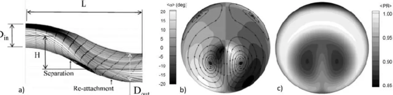
DVANCED propulsion system installations for current and future aero vehicle architectures feature short and complex intake configurations where the coupling with the engine becomes critical1,2. Previous work showed that complex engine intakes are notably susceptible to flow separations and large unsteady perturbations, which can potentially compromise the operability of the entire propulsion system3-6. Examples of flow non-uniformities at the exit of a complex intake are presented in Fig. 1 which shows the computed time averaged total pressure and swirl angle distortion distributions7. These are results from Reynolds Averaged Navier Stokes (RANS) based simulations for an S-duct with an area ratio Aout/Ain=1.52 and offset to inlet diameter ratio H/Din=1.34 which was also previously studied experimentally by Wellborn et al8. These previous works indicate a flow separation within the first bend of the S-duct (Fig. 1a) which interacts with the associated secondary flows and results in two counter-rotating vortical structures located at the lower part of the AIP (Fig. 1 b, c). These are further highlighted by the flow path lines superimposed on the swirl angle and pressure recovery contours of Fig. 1. The unsteady behaviour of these types of flow fields and the associated unsteady swirl and pressure distortions were further analysed by Chiereghin et al7, MacManus et al9 and Garnier et al10,11. These works highlight the need for spatially and temporally rich and synchronous datasets to enable the assessment of total pressure and swirl distortion for operability assessments.
Although current industry practice typically relies on low spatial resolution intrusive rakes for the measurement of the pressure and swirl distortion patterns these were found to be unable to capture the complex nature of the flows
A
Figure 1. Example of the flow field for a convoluted S-duct calculated using a steady RANS simulation. (a): surface streaklines (b): swirl angle and (c): total pressure ratio at the AIP7.
3
in both the spatial and the temporal domain3. This limitation of the intrusive swirl distortion measurement systems can be addressed by applying Stereoscopic Particle Image Velocimetry (S-PIV) techniques for the measurement of the AIP velocity fields. This approach has the potential to provide 200-300 times higher spatial resolution than the conventional intrusive rakes across a typical AIP in a synchronous way and enables three component, planar velocity measurements. These can then be used to evaluate swirl distortion metrics at each flow snapshot as well as to evaluate the distortion statistics over a period of time. This method was successfully applied for AIP velocity field measurements at the exit of complex intakes across a range of inlet Mach numbers as reported by Zachos et al12.
However, the need for total pressure distortion characterisation still remains as S-PIV systems only provide velocity measurements. A potentially attractive approach to establish a direct link between swirl distortion measurements and the associated pressure distortion could be through the reconstruction of the underpinning AIP static pressure field by using velocimetry data. This way the advantages of the S-PIV synchronous and spatially rich velocity fields could be further exploited for the derivation of the pressure distortion characteristics associated with them. Furthermore, apart from the inherent synchronisation of pressure and velocity information, such an approach removes the need for additional intrusive instrumentation to measure pressure distortion.
Pressure field reconstruction from velocity data techniques are relatively well known and have been applied to determine integral aerodynamic forces and moments in fluid-structure interactions. Several of these methods have been proposed to enable the coupling of the pressure fields with the associated mechanical loads as reported by Lin and Rockwell13, Unal et al14, Noca et al15,16 and Fujisawa et al17. These methods have been developed to support aerodynamic load determination in applications investigated using velocimetry techniques and to allow the synchronous estimation of flow and load information. For temporally resolved PIV data, these methods often permit flow acceleration terms to be determined with a sufficient level of accuracy as discussed by van Oudheusden et al in18,19 and Hosokawa et al20.
The aim of this work is to apply pressure field reconstruction methods in order to characterise the total pressure distortion generated by complex engine intakes using velocity information. Pressure fields are reconstructed by means of Direct Spatial Integration (DSI) of the momentum equation14,19 as well as by integration of the Poisson Pressure Equation (PPE) as proposed by Fujisawa et al17 and Hosokawa et al20. Velocity data from unsteady Computational Fluid Dynamics (CFD) simulations are used for the AIP pressure field reconstruction for a typical S-duct configuration with an offset to inlet diameter ratio H/Din=2.44, area ratio Aout/Ain=1.52 across a range of inlet Mach numbers Min between 0.27 and 0.6. The Reynolds number ranged from 0.7×10⁶to 1.4×10⁶. The generated
pressure fields are then used for the calculation of the total pressure distortion metrics and the results are compared against pressure field distributions and distortion metrics directly calculated from the CFD data. The effects of temporal and out-of-plane velocity gradients on reconstruction accuracy are assessed with the aim of determining the applicability of time-resolved, stereoscopic PIV systems for steady and unsteady pressure distortion characterisation of the flow at the exit of a complex intake.
II.
Theoretical background and methods
A. Governing equations
For the calculation of the pressure field the incompressible momentum equation was used in conservative form as follows:
∇p = −ρ + ∙ ∇ + μ∇ (1)
Eq. (1) was solved in cylindrical coordinates on the AIP plane (Fig. 2) at the exit of the S-duct intake with diameter DAIP=150 mm. A polar grid was used to discretise the computational domain (Fig. 2) with a total of 9,000 nodes arranged in 50 equi-spaced rakes and 180 equi-spaced circumferential rings. This spatial resolution is similar to that achieved by S-PIV measurements of the same S-duct configuration (H/Din=2.44, DAIP=150 mm) reported by Zachos et al12. Considering a two dimensional, incompressible and inviscid flow at the AIP and assuming that the contribution of the diffusive terms is negligible as stated by van Oudheusden et al19, the spatial pressure gradients can be estimated in cylindrical coordinates as follows:
= − + + − + (2)
Eqs. (2) and (3) allow the derivation of the AIP spatial pressure gradients using only spatial and temporal velocity gradients, after which the pressure can be obtained from integration. A circumferential static pressure distribution along the outer boundary of the domain is required as a boundary condition to allow the calculation of the pressure field across the entire domain of interest.
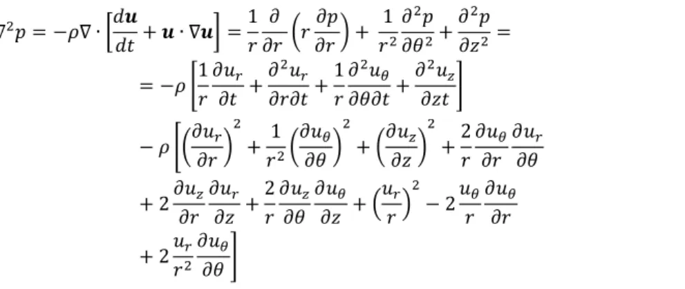
Alternatively the spatial pressure gradient may also be obtained through solving the Poisson Pressure Equation which is derived from the inviscid form of Eq. (1) by applying the divergence operation as follows17:
(4) To solve Eq. 4 in the polar domain (Fig. 2), a prescribed static pressure distribution along the outer boundary of the domain would normally suffice. This would be similar to the one used to solve Eqs. (2) and (3). However, in order to avoid singularities in the numerical integration scheme, the centre of the computational domain (r=0) is removed. This yields to the necessity of a virtual boundary within the domain which requires a second boundary condition. The virtual boundary however cannot be treated with a Dirichlet boundary condition as the static pressure is unknown in this region. Hence, a Neumann type boundary condition is required whereby the divergence of the static pressure along the virtual boundary must be prescribed as:
∇ ∙ = at Ω (5)
where Ω is the computational domain, Ω the domain virtual boundary (Fig. 2), n the outward unit vector normal to
Ω and g a known function along the domain boundary. Eq. (5) finally reduces to − = which can then be calculated by Eq. (2) based on velocity data.
To introduce compressibility effects a possible solution would be to use the continuity equation to directly derive density at each node. However, as reported by van Oudheusden et al19 this method was found to introduce errors in
∇ = − ∇ ∙ + ∙ ∇ =1 + 1 + =
= − 1 + +1 +
− + 1 + +2
+ 2 +2 + − 2 + 2
Figure 2. Domain discretization at a given axial position k and boundary conditions of the computational domain used for the reconstruction of the pressure field at the exit of a complex engine intake.
5
the pressure field reconstruction. A simpler method to estimate flow density was used herein based on the adiabatic flow condition and the ideal gas law19. The gas law is employed to replace the density in the momentum equations where the static temperature is derived from the assumption of constant total enthalpy using the velocity magnitude at each node as follows:
, = , ; = − , (6) B. Reconstruction numerical method
The radial and circumferential velocity gradients involved in the DSI and PPE total pressure reconstruction methods (Eqs. (2),(3) and (4)) were approximated using a central finite difference scheme as follows:
, , = , , , , ∆ + O(∆ ) ≈ , , , , ∆ (7) , , = , , , , ∆ + O(∆ ) ≈ , , , , ∆ (8) , , ≈ , , , , ∆ (9)
where ui refers to a generic velocity component and Δr, Δθ and Δz are the grid spacing in the radial and
circumferential and out-of-plane (streamwise) directions respectively. For the calculation of the temporal velocity gradients the following expression was used:
, , ≈
, , ∆ , , ∆
∆ (10)
For the reconstruction of time averaged pressure fields, the temporal velocity gradients were all set to zero and velocity data from the time average field was used in Eqs. (2), (3) and (4)20.
For the integration of the pressure gradients across the domain the space marching technique reported by Baur and Koengeter21 was used. For the calculation of the static pressure at any given node, four already calculated pressure values from neighbouring nodes are used as integration paths to evaluate an average static pressure at given cross-flow plane k as follows:
, = , + Δ , + , + Δ , + , + Δ , + ( , + Δ , ) (11)
The calculation proceeds towards the inner domain starting from the external far field boundary where the static pressure is known. A first order Taylor’s polynomial is used to evaluate the pi+Δpi terms across the plane as follows:
, + Δ , = , +
, ∆ , + , ∆ , (12)
The spatial pressure gradient components and are calculated based on velocity data using Eqs. (2) and (3). For solving the Poisson Pressure Equation (Eq. (4)), the left hand side pressure terms are discretized using second order central derivatives as follows:
∇ , , = + + , , ≈ , , , , , , + , , (∆ ), , , , + , , , , , , , , (∆ ) + , , , , , , (∆ ) (13)
The spatial and temporal velocity derivatives that appear at the right hand side terms of Eq. (4) are discretized using Eqs. (7), (8), (9) and (10). The static pressure at each grid node across the computational plane is explicitly determined as:
, , = ∆ , , ∆ , , , , , , + , (∆ ), , , + , , , , , , (∆ ) − , , (14)
where fi,j,k is the known velocity based term from Eq. (4). Eq. (14) is solved using an iterative Gauss-Seidel
method22. A successive over-relaxation factor was introduced to accelerate convergence. The domain was initialised with a static pressure distribution obtained from Eq. (6) and constant density applied across the AIP.
C. Computational methods 1. CFD method
The unsteady CFD calculations are performed using a Delayed Detached-Eddy-Simulation (DES) with the k-ω SST turbulence model. A pressure-based solver was used with a segregated PISO scheme23. The pressure spatial gradients were solved using a second-order scheme and a third order MUSCL scheme was used for momentum, energy and turbulence. The steady RANS simulations were performed using the same methods with the k-ω SST turbulence model. For the unsteady DDES simulations, the temporal discretisation was addressed using a bounded second-order method23. The inlet boundary condition comprised specified uniform total pressure and total temperature profile. The static pressure was specified at the domain exit and was adjusted to provide the required average Mach number at the inlet.
The overall duct domain was discretised using a multi-block structured mesh. The baseline mesh had 5 million nodes. The mesh had a H-grid structure in the central part of the duct, and an O-grid structure around the wall which resulted in a good quality mesh as indicated by a 2x2x2 determinant greater than 0.8. The near wall boundary layers were resolved with a structured mesh which provided y+ less than 1 over the full domain. Previous work9 using this method for the same S-duct configuration, at a slightly greater Reynolds number, evaluated the mesh independence using grids of 3.1, 5.9 and 11.2 million nodes. For the unsteady DDES calculations the time step was adjusted to ensure similar Courant number for the different meshes. Between the medium and fine mesh the changes in time-averaged pressure ratio (P0/P0,ref) was less than 0.1% along with a 5.7% reduction in the temporal standard deviation
of PR. The distortion metrics were more sensitive to the mesh resolution although they are not conserved thermodynamic properties. The time averaged metrics for swirl and total pressure distortion changed by up to approximately 6% respectively between the medium and fine mesh configurations.
2. Computational time steps
A time step ∆t of 6x10⁻⁶ s was chosen for the Min=0.6 cases which corresponds to a non-dimensional time step ∆t of approximately 0.0018 with respect to the mean overall convective time through the duct. Previous work9 investigated the effect of the time step for the Min=0.6 configuration which was also simulated with a time step of 12x10-6 s and the time average and unsteady swirl and total pressure distortion metrics were compared. The results showed that the time-averaged values of the distortion metrics were changed by up to 3% with the time step reduction from 12 to 6x10⁻⁶ s. The unsteady characteristics were more sensitive to the change in time step with variations of standard deviation by up to 7% with this time step reduction.
In this work the DDES calculations used 20 sub-iterations per time step which typically resulted in residuals in the order of 10-6 for continuity equation and 10-7 for momentum, energy, k and ω equations, with a reduction of at least three orders of magnitude of all the residuals for each time step. For all the cases, a discarded interval of 15 convective times where used as a transition between the steady solution and the established unsteady flow field. 3. CFD validation
The CFD method adopted in this study was previously validated based on experimental data for the same S-duct geometry but at a slightly increased size and Reynolds number9. The Mach number range was the same as considered here as Min=0.27 to 0.6. Overall the time averaged total pressure ratio agreed exactly with the measurements. The maximum unsteady PR typically agreed within 5% of the measured data. Overall, the DDES method has been examined and validated to demonstrate that it is capable of simulating these types of flow fields. Consequently, in the assessment of the pressure reconstruction methods, the DDES data is an appropriate source of high-resolution, representative data. For the reconstruction analyses in this current work the CFD data at the AIP was extracted and interpolated, by Kriging, onto a uniform polar grid with 50 radial and 180 circumferential points.
7
III.
Results and discussion
A. Time averaged pressure field reconstruction
The first assessment of the reconstruction methods was performed by considering a steady flow field. The steady total pressure reconstruction methods was carried out using numerically calculated pressure and velocity data from steady RANS simulations. The steady total pressure recovery AIP distributions are shown in Fig. 3 for Min=0.6. The DSI based mean static pressure field was calculated from average velocity flow field data at the AIP by averaging the instantaneous momentum equations (Eqs. (2) and (3)). PPE based static pressure fields were reconstructed from the steady Poisson pressure expression (Eq. (4)). The total pressure at the AIP nodes was calculated from the isentropic pressure relation (Eq. (6)) and the reconstructed static pressure values as:
= (1 + ) (15)
In order to assess the mean total pressure field reconstruction accuracy, the difference between the reconstructed
(p0,rec) and the RANS calculated total pressure (p0,CFD) was determined at each point across the AIP as:
∆ = , ,
, (16)
The accuracy of a pressure reconstruction algorithm was reduced to a single index defined across the AIP as:
=
∑ ∑ ( )
∙
(17) where q is the mean dynamic head at the inlet of the S-duct defined as = with ρ the flow density and Uin
the meanline flow velocity at the inlet. Index I is useful when comparing between different pressure reconstruction methods as it represents the non-dimensional root mean square of the average reconstruction error across the domain.
Distributions of the reconstructed total pressure ratio (p0/p0,ref) at the AIP located 0.296Din downstream the S-duct
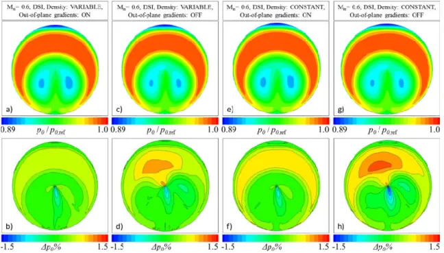
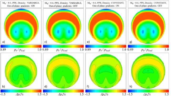
exit plane as well as the discrepancy from the time averaged RANS computed total pressure field are shown in Fig. 4 and Fig. 5. This is for the high offset S-duct (H/Din=2.44) at an inlet Mach number Min of 0.6 defined at a reference plane 0.934Din upstream the S-duct inlet. These reconstructions use the DSI scheme for various combinations of treatment for the density and out-of-plane velocity gradient terms. For the total pressure field reconstructions the static pressure distribution imposed along the domain boundary was obtained from the RANS simulations.
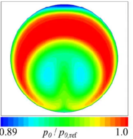
Figure 3. RANS computed steady AIP total pressure recovery distribution for the S-duct with H/Din=2.44. at Min=0.6.
For the reconstruction with variable density and the terms included, the reconstructed total pressure distribution (p0/p0,ref) exhibits the main features of the original data (Fig. 4a). The error is relatively uniformly
distributed across the AIP with peak values in the order of ±0.7% (Fig. 4b). For the same base flow field and when the term was neglected in the reconstruction, the broad topology remained the same (Fig. 4c) and the peak error increased to approximately 1% (Fig. 4d). Relative to the baseline DSI reconstruction case (Fig. 4a), the impact of the density terms showed that for the case with a constant density (Fig. 4e, f) there is a very slight increase in the error which predominately affects the upper sector of the AIP where it increases from 0.7% to 1.2%. Finally, the overall combined effect of assuming a constant density as well as a = 0 gives the worst result although the peak error is approximately 1.5%. The same characteristics are reflected in the I-index (Table 1), whereby the effect
of the term is relatively more important than the treatment of the density. However, the level of the errors is still relatively low with I in the region of 0.017 for the worst case. This finding is pertinent to pressure field reconstruction when planar experimental velocimetry data is available, such as reported by Zachos et al12, which do not enable the calculation of the out-of-plane velocity gradients.
The PPE integration approach also has an impact on the reconstruction and the relative sensitivities to the treatment of the density and terms (Fig. 5). Overall, the PPE approaches also reconstruct the same general
p0/p0,ref topologies (Fig. 5) in comparison with the DSI method (Fig. 4) and the original time averaged flow (Fig. 3).
For the configuration with variable density and including the terms, the peak error for the PPE method very slightly increases to 1.1% (Fig. 5b) relative to the same assumptions using the DSI method which had a peak error of 0.7% (Fig. 4b). Overall for all of the PPE cases, the reconstruction accuracy remains in the region of 1.1%. Relative to the DSI method, the PPE approach is less sensitive to the effects of changes to the treatment of density and (Fig. 5). When = 0 the maximum error is generally unaffected although there is a very slight decrease in I-index from 5.3x10⁻³ to 5.6x10⁻³ (Fig. 5b, d, Table 1). When density is held constant (Fig. 5f, h) the effects are even less pronounced with a small decrease in I from 5x10⁻³ to 4.8x10⁻³ (Fig. 5b,f, Table 1).
Figure 4. Steady DSI reconstruction for the S-duct with H/Din=2.44 at Min=0.6. Top row: time averaged
9
Table 1. Accuracy index I for reconstructed steady total pressure fields.
DENSITY Ix10 3 Min=0.6 Ix103 Min=0.27 DSI variable on 6.7 6.4 variable off 15 16 constant on 6.8 6.5 constant off 15 17 PPE variable on 5.3 5.5 variable off 5.6 6.5 constant on 5 5.5 constant off 4.8 6.5
Pressure field reconstructions at a lower inlet Mach number of 0.27 were conducted with both the DSI and PPE, methods. Relative to the Min=0.6 cases, the error in the total pressure fields at the AIP reduced to approximately ± 0.2% when the out-of-plane gradients were accounted for. When = 0, the error marginally increased to 0.6% across the AIP. Based on the accuracy index I, the low Mach cases (Table 1) show that for both the DSI and PPE methods the errors are broadly independent of Min across this range. In addition, the sensitivity to treatment of density and the out of plane velocity gradient is similarly relatively independent to Mach number.
Overall, both the DSI and PPE based pressure reconstruction methods were found to perform sufficiently well for steady field reconstruction based on velocity data. Total pressure fields obtained by the PPE integration provide slightly more accurate reconstructions relative to the DSI method across the range of Min and are less sensitive to changes to the treatment of density and terms. Given that broadly the discrepancies of both methods remain
Figure 5. Steady PPE reconstruction for the S-duct with H/Din=2.44 at Min=0.6. Top row: time averaged
at very low levels regardless of the treatment of the out-of-plane velocity gradient or density terms, it can be concluded that in principle these procedures could potentially allow the derivation of steady field data from planar, 3-component, PIV measurements with sufficient level of accuracy. The effect of the reconstruction on the conventional flow distortion metrics is considered in Section C.
B. Unsteady pressure field reconstruction
Delayed Detached Eddy Simulations (DDES) provided time histories of the flow field through the S-duct for the configuration with Min=0.6. The simulations showed a highly dynamic flow in which the topology of the total pressure and velocity flow field at the AIP varied significantly with large changes in the distortion metrics7,9. Furthermore, both the total pressure and swirl distortion at the AIP was calculated to be substantially different from the symmetric time-averaged flow field. Consequently, the wide range of flow field characteristics and features which arise from the DDES simulations provide a robust test for the unsteady reconstruction methods considered in this work. The DDES simulation time step was Δt was 6x10⁻⁶ s with the solution saved every 3 time steps which results to a time interval of 18x10-6s between two subsequent solutions. This equates to a velocity sampling rate of 55kHz. From the full DDES simulation, a representative set of 100 timesteps were used to provide a sample of dynamic distortion fields for the assessment of the proposed reconstruction methods.
For this set of unsteady flow field data at the AIP, the methods to reconstruct the pressure field from the 3 components of velocity were evaluated. The accuracy of the unsteady total pressure reconstruction methods considered the variable density DSI approach and the impact of out of plane velocity gradients as well as temporal velocity gradients (Table 2). The metric to quantify the overall reconstruction tools is the averaged root mean square error defined in Eq. (17) as:
= ∑ (18)
where n is the total number of instantaneous flow fields considered.
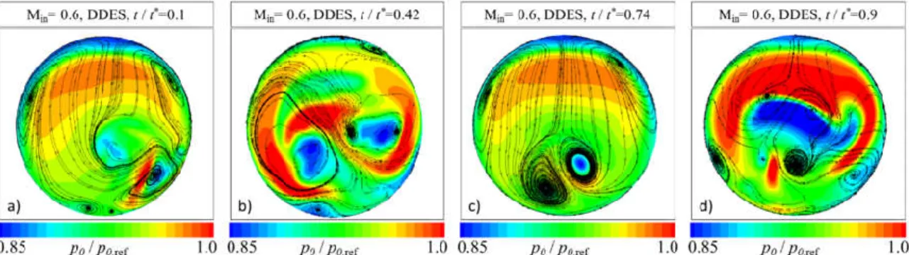
Fig. 6 shows instantaneous total pressure ratio (p0/p0,ref) distributions at the AIP for four different normalised
time instances across a range between t/t*=0.1 and 0.9 where t*=100x1.8 μs. Fig. 6 highlights the remarkable flow
non-uniformities across the AIP for a given timestep as well notable changes over time. As discussed by MacManus et al9 steady state or even unsteady RANS calculations are unable to reveal the complex underpinning aerodynamic structures of the flow fields. In addition, low bandwidth and low resolution distortion rakes, typically 8x5, can hardly provide the required spatial and temporal resolution to sufficiently measure these flow fields experimentally. Numerical methods of higher fidelity, such as unsteady DDES, or experimental techniques capable of delivering sufficiently high spatial and temporal resolution such as S-PIV or time resolved S-PIV are better positioned to capture the complexity of the underpinning flow mechanisms7,9.
Fig. 7 and Fig. 8 show reconstructed total pressure fields using the unsteady DSI method as well as the relative discrepancies from the full DDES solution (Eq. (16)). For the reconstruction of the pressure fields shown in Fig. 7 the out-of-plane and temporal velocity gradients , are included in the analysis. The relative effect of excluding these terms is shown in Fig. 8. This is pertinent when total pressure reconstruction is attempted based on time resolved, tomographic velocimetry data. The flow density was set as variable in both cases. The total pressure fields generated using the unsteady DSI approach show a discrepancy within a typical range of ±0.5% which locally increases up to ±1.8% from the correspondent DDES flow snapshots (Fig. 7). The DSI algorithm demonstrated notable robustness in reconstructing the pressure fields of the different instances of the unsteady velocity fields despite the high rates of velocity gradients in both the circumferential and radial directions of the AIP.
A numerical experiment was conducted using the unsteady DSI reconstruction method and neglecting the out-of-plane and temporal velocity gradients . The rationale for this numerical experiment was to identify the extent to which the omission of the and terms compromises the calculation of the pressure gradients (Eqs. (2) and (3)). This is pertinent to unsteady total pressure field reconstructions when only low temporal resolution, single-plane velocity data is available. If only temporally under-resolved velocity data is available, inclusion of the terms into the static pressure calculation (Eqs. (2) and (3)) would produce erroneous calculation of the static pressure gradients24. Hence the current investigation aims to quantify for this type of flow
11
field the fidelity of the pressure field reconstruction for the terms neglected from the calculation. A rigorous study on the identification of the temporal resolution required for the velocity data to generate representative static pressure fields around an airfoil located downstream of a circular rod was conducted by Violato et al24. This study reports an estimate of the maximum time interval between two subsequent velocity fields, Δt, above which the static pressure gradients of Eqs. (2) and (3) cannot be representatively evaluated due to erroneous calculation of the flow acceleration. The outcome of Violato’s studies24 showed the effect of the unsteady velocity acquisition rate on the evaluation of the flow accelerations included in the pressure reconstruction equations for external flows considered. This is pertinent to the determination of an appropriate setup for an unsteady velocity measurement method such as time-resolved planar S-PIV or tomographic PIV.
Reconstructed total pressure fields using the unsteady DSI method are shown in Fig. 8 where the out-of-plane and temporal velocity gradients have been neglected. These reconstructed total pressure fields result in local maximum differences from the DDES original data of up to ±8% .This is notably higher than the 1.8% maximum discrepancy when the out-of-plane and temporal terms are included (Fig, 7). The mean accuracy index for each case (Table 2) highlights this loss in fidelity as increases from 9x10⁻³ to 49x10-3 when the out-of-plane and the temporal terms are both neglected. However, in spite of this relative increase in the error, this simplified unsteady DSI reconstruction generates total pressure fields whose main characteristics are representatively captured in comparisons with the original field (Fig. 6). This suggests that useful total pressure field reconstructions may be feasible from planar, temporally under-resolved velocity information, despite the accuracy penalty introduced by the lack of streamwise and temporal velocity gradients. The next section assesses this aspect through an evaluation of the reconstructed flow distortion metrics.
Table 2. Average accuracy index for unsteady DSI reconstruction for the S-duct at Min=0.6.
10 Min=0.6
DSI on on 9
DSI off off 49
C. Total pressure distortion metrics reconstruction 1. Steady reconstruction
Current industry practice for the assessment of flow distortion typically relies on steady state experimental measurements for the quantification of distorted flow fields for compressor or fan systems4,5. These allow the characterization of distortion through a set of distortion descriptors. A standard measurement arrangement for advanced engine intakes uses a total pressure rake at the AIP comprising an array of 8 spokes with 5 probes each (Fig. 9). To assess the total pressure distortion a range of descriptors is typically considered and the calculations are based on a “ring and rake” approach (Fig. 9). The total pressure recovery coefficient (PR = P0, AIP / P0,in) is
Figure 6. Instantaneous total pressure fields predicted from DDES simulations for the high offset S-duct (H/Din=2.44) at Min=0.6.
also a property of interest. The circumferential distortion index (CDI) assesses the uniformity of the circumferential total pressure distribution and is defined as follows25:
Figure 7. Unsteady DSI total pressure field reconstruction and discrepancy from DDES. Out-of-plane and time derivative terms included. S-duct with H/Din=2.44 at Min=0.6.
Figure 8. Unsteady DSI total pressure field reconstruction and discrepancy from DDES. Out-of-plane and time derivative terms neglected. S-duct with H/Din=2.44 at Min=0.6. Contours limited to be consistent
13
CDI = Max 0.5 , ,
, +
, ,
, (19)
where p , is the average total pressure, p , the average total pressure of the pressure distribution of the i-th ring and p , the minimal pressure of the i-th ring. Finally the radial distortion can be assessed by the radial distortion index (RDI). The formula follows the same logic as CDI and is defined as follows25:
RDI = Max , ,
, ,
, ,
, (20)
where p , is the average total pressure of the pressure distribution of the inner ring and p , is the average total pressure at the outer ring. Finally, DC(60) is an overall distortion metric which is defined as the difference between the average total pressure, p0,avg, and the lowest average total pressure in a sector of 60° angle,
p60o,avg and non-dimensionalized by the mean dynamic head q of the AIP25.
DC(60) = , , ° , (21)
where p , is the mean total pressure and p , ° , is the mean total pressure measure in a sector of 60 degrees. The total pressure distortion descriptors calculated from the time average, RANS predicted pressure fields for the high offset configuration across a range of inlet Mach numbers is shown in Table 3 and Table 4.
In this work an 8x5 rake and ring arrangement was used for the distortion descriptors calculation using CFD and reconstructed pressure fields (Fig. 9). Pressure recovery and distortion characteristics calculated based on the time averaged RANS predicted flow fields are summarised in Table 3 and Table 4 for the S-duct at Min=0.6 and Min=0.27 respectively.
The distortion metrics calculated from the reconstructed steady total pressure fields for both the DSI and PPE approaches (Fig. 4 and Fig. 5) are summarised in Table 3 and Table 4 for the Min=0.6 and 0.27 cases. The discrepancy between the reconstructed values and the values calculated directly from the original RANS pressure fields is also shown. This is calculated as:
= (22)
where xrec is the metric of interest (Eq. (19) to (21)) calculated from the reconstructed pressure data and xCFD the
same property based on the original CFD pressure field.
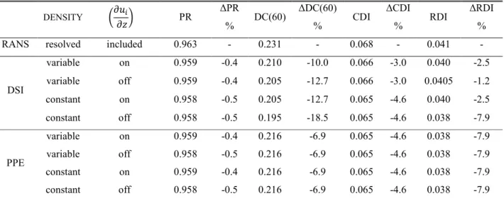
Both the steady DSI and steady PPE reconstructed total pressure fields show a relatively accurate calculation of PR with a discrepancy from the RANS based value not higher than 0.1% (Table 3). The out-of-plane velocity gradients have no impact on the PR reconstruction fidelity, while the discrepancy in PR only slightly increases from -0.4% to -0.5% for total pressure fields reconstructed with constant density across the whole domain. At Min =0.6, all of the distortion descriptors, DC60, RDI and CDI, are underestimated by both methods and for various combinations of out of plane gradients and density assumptions. These errors range from -1.2% to 18.5%. DC(60) is under-estimated by both DSI and PPE reconstruction approaches with the highest discrepancies from the
constant density DSI approach where, neglecting , the error is -18.5% (Table 3). This reduces to -10% when the variable density and terms are included.
PPE reconstructed total pressure fields under-estimate the DC(60) by around -7% relative to the RANS data (Table 3). This under-prediction is not affected by the out-of-plane terms and remains constant when the total pressure field is reconstructed with constant density. CDI is consistently under-predicted by both PPE and DSI by around 3-5% relative to the RANS data and is relatively insensitive to the out-of-plane gradients or treatment of density. Finally, RDI is also under-estimated by both methods with a relative error of between -1.2% and -7.9% although the absolute differences are small. PPE and DSI are broadly insensitive to density and terms except for the DSI method where the error increases from -2.5% to -7.5% when these terms are neglected.
Total pressure distortion descriptors were reconstructed for Min=0.27 using both DSI and PPE methods and variable density across the AIP (Table 4). At this lower Min the original total pressure ratio (P0, AIP / P0,in) increases
from 0.963 to 0.998 although there DC60 distortion metric only slightly changes from 0.231 to 0.223. At this lower Mach number, and also partially due to the definition of the terms, both CDI and RDI are substantially reduced from 0.068 and 0.041 to 0.013 and 0.008, respectively. Both the DSI and PPE methods reflect the changes in PR and there is a no difference between the reconstructed and original data for PR, CDI and RDI (Table 4). At this lower Mach number the difference on DC60 has reduced for both the DSI and PPE methods. The PPE is still insensitive to the terms and typically overestimates DC60 by up to 2%. The DSI approach is more sensitive to these terms and the error ranges from about -4 to -11%.
Table 3. Reconstructed steady distortion metrics and discrepancy from RANS simulations. High offset S-duct at Min=0.6. DENSITY PR ΔPR % DC(60) ΔDC(60) % CDI ΔCDI % RDI ΔRDI %
RANS resolved included 0.963 - 0.231 - 0.068 - 0.041 -
DSI variable on 0.959 -0.4 0.210 -10.0 0.066 -3.0 0.040 -2.5 variable off 0.959 -0.4 0.205 -12.7 0.066 -3.0 0.0405 -1.2 constant on 0.958 -0.5 0.205 -12.7 0.065 -4.6 0.040 -2.5 constant off 0.958 -0.5 0.195 -18.5 0.065 -4.6 0.038 -7.9 PPE variable on 0.959 -0.4 0.216 -6.9 0.065 -4.6 0.038 -7.9 variable off 0.958 -0.5 0.216 -6.9 0.065 -4.6 0.038 -7.9 constant on 0.959 -0.4 0.216 -6.9 0.065 -4.6 0.038 -7.9 constant off 0.958 -0.5 0.216 -6.9 0.065 -4.6 0.038 -7.9
Table 4. Reconstructed steady distortion metrics and discrepancy from RANS simulations. High offset S-duct at Min=0.27. DENSITY PR ΔPR % DC(60) ΔDC(60) % CDI ΔCDI % RDI ΔRDI %
RANS resolved included 0.998 - 0.223 - 0.013 - 0.008 -
DSI variable on 0.998 0 0.215 -3.7 0.013 0.0 0.008 0.0
variable off 0.998 0 0.201 -10.9 0.013 0.0 0.008 0.0
PPE variable on 0.998 0 0.228 2.2 0.013 0.0 0.008 0.0
15
The analysis on the descriptor reconstruction for steady data shows that generally the two reconstruction approaches offer broadly the same level of accuracy in descriptor estimation across the range of Min except for DC(60). DC(60) is under-estimated by a maximum of almost -20% by the DSI approach while PPE under-estimates by -7% for Min=0.6 when the out-of-plane velocity gradients are not accounted for in the calculations. These errors reduce to -11% and 1% respectively for Min=0.27. These assessments give an indication of the uncertainty in steady total pressure distortion descriptors based on planar, mean flow velocity data such as that from planar S-PIV measurements. A measured velocity dataset which includes the out-of-plane velocity terms, such as from tomographic PIV experiments, would provide higher confidence in the total pressure descriptors. However, for this steady flow, the benefits are very small.
2. Unsteady reconstruction
Unsteady velocity and wall static pressure data from the DDES simulations was used to reconstruct the total pressure field and to calculate the total pressure ratio (P0, AIP / P0,in) as well as the pressure distortion descriptors for
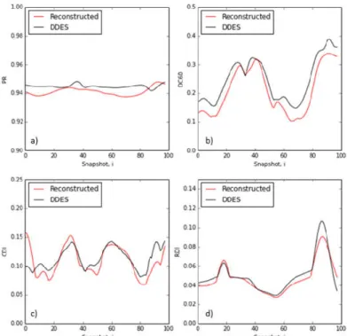
each time step. The DDES data was also used to calculate the same parameters based on the original CFD distributions of total pressure and thereby enable an assessment of the unsteady DSI reconstruction method. The distortion descriptors were evaluated based on a typical 8x5 rake resolution at the AIP (Fig. 9). Fig. 10 and Fig. 11 show the comparison between the unsteady distortion metrics calculated directly from DDES data against those calculated from the DSI reconstructed unsteady total pressure fields for the S-duct at Min=0.6. The accuracy of the reconstructed descriptors is quantified by means of the root mean square discrepancy from the DDES based values as:
= ∑ ( ) (23)
where n is the total number of snapshots and Δx defined in Eq. (22).
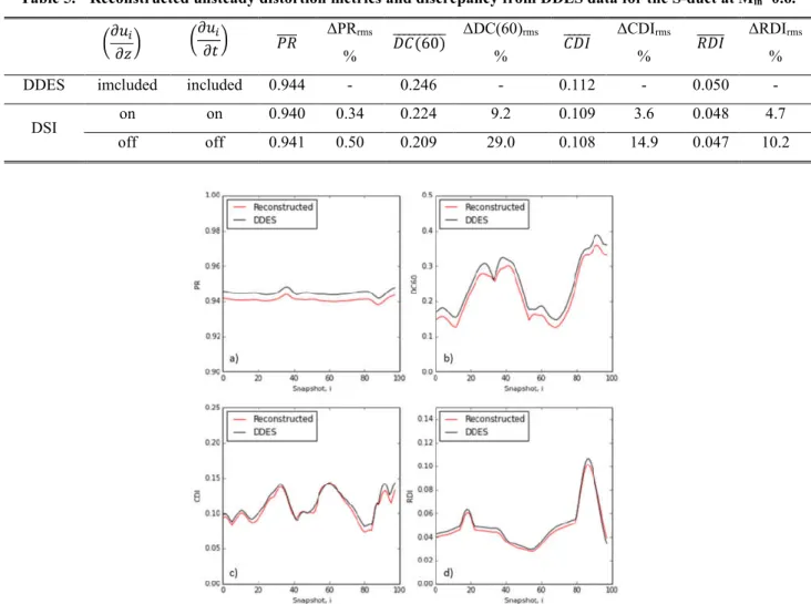
Fig. 10 shows the temporal variation of the distortion descriptors from the original DDES data as well as for the DSI reconstructed total pressure fields with out-of-plane and temporal gradient terms included. PR, CDI and RDI reconstruction shows an rms discrepancy from the original DDES data of 0.42%, 3% and 4%, respectively (Fig. 10a, c, d, Table 5). The DC(60) time history is slightly more under-estimated by approximately 9% (Fig. 10b). For this dataset, the PR exhibits very little variation with time-step although there are more notable variations in the distortion descriptors particularly for DC60 and RDI. Overall, the reconstruction method clearly follows the temporal characteristics of the descriptors and captures the local maxima and minima with particularly good agreement in RDI and CDI (Fig. 10c, d).
The reconstructed unsteady pressure recovery and distortion descriptors using the DSI method are susceptible to uncertainties imposed by the out-of-plane and temporal velocity changes . These uncertainties are more pronounced in DC(60), CDI and RDI while PR is generally less affected by these terms. The errors for CDI and RDI increase to 15% and 10%, respectively, while ΔPRrms% remains below 1% (Table 5). In addition, ΔDC(60)rms% increases to approximately 30% from about 9% previously (Table 5, Fig. 11). When these terms are neglected, although the error increases, the reconstructed time history of the distortion descriptors still reproduces the main unsteady aspects and temporal changes in the metrics (Fig. 11).
A time resolved, tomographic PIV system can potentially provide both spatial and temporal information that is required to apply the unsteady DSI method and therefore the uncertainties and characteristics highlighted in Fig. 10 and Table 5 could be expected for this type of flow field. However, a planar, temporally under-resolved measurement system is less complicated and can provide potentially useful distortion assessments, albeit at a reduced accuracy. Overall, descriptor reconstruction with steady, planar velocity data seems to be susceptible to around 30% error in terms of DC(60) while PR, CDI and RDI show a maximum departure from the original DDES based values of approximately 15%.
D. Effect of boundary conditions
For the reconstruction of the steady total pressure fields (Fig.4, Fig. 5) a static pressure distribution was imposed along the outer boundary grid nodes of the domain (Fig. 1). This boundary condition was obtained from the numerical simulations and comprises approximately 200 points which is equivalent to the azimuthal computational grid resolution. For the reconstruction of the unsteady total pressure fields (Fig. 7 and Fig. 8) the boundary static pressure profile was updated for each time step from the respective unsteady DDES data. Hence, the unsteady total pressure field reconstruction was performed using a temporally synchronous static pressure boundary condition with
the velocity field. However, it is pertinent to examine the behaviour of the pressure reconstruction algorithms in relation to the number and nature (steady or unsteady) of the static pressure imposed along the boundary of the domain. The outcome of this investigation quantifies the fidelity of the total pressure reconstruction methods when the boundary condition is experimentally measured from circumferentially located wall static pressure tappings.
Fig. 12 shows the normalised steady wall static pressure distribution of the RANS predicted flow field for the
S-duct configuration at Min=0.6 (Fig. 3b) as well as the approximation of this distribution using 6 or 18 equi-spaced circumferential data points from the same set of numerical simulations. A circumferential resolution of 6 wall static pressure values is insufficient and, for this example, a spatial resolution of 18 points is required to sufficiently capture the local maximum (Fig. 12)
The effect of boundary spatial static pressure resolution on the steady total pressure distortion metrics is shown in Table 6 for the S-duct configuration at Min=0.6. For this example, PR, CDI and RDI are insensitive to the circumferential resolution. It has, however, a more notable impact on DC(60) which is over- predicted by around 10% with 6 points but under predicted by -11% with 18 circumferential points.
The behaviour of the unsteady DSI total pressure reconstruction method was assessed for different spatial resolution of static pressure tappings along the domain boundary. A variable density, unsteady DSI approach was used for the total pressure reconstructions with the out-of-plane and temporal velocity gradients enabled. The impact of the number of boundary static pressure points on the unsteady reconstruction accuracy was
Figure 10. Unsteady distortion metrics and discrepancy from DDES. Unsteady DSI with out-of-plane and time gradients enabled. (a): PR, (b): DC(60), (c): CDI and (d): RDI. S-duct with H/Din=2.44 at
Min=0.6.
Table 5. Reconstructed unsteady distortion metrics and discrepancy from DDES data for the S-duct at Min=0.6.
ΔPRrms % (60) ΔDC(60)rms % ΔCDIrms % ΔRDIrms %
DDES imcluded included 0.944 - 0.246 - 0.112 - 0.050 -
DSI on on 0.940 0.34 0.224 9.2 0.109 3.6 0.048 4.7
17
assessed for the S-duct at Min=0.6. Steady as well as unsteady boundary static pressures were applied. The rationale for the latter is a scenario whereby synchronous, unsteady wall static pressure measurements are acquired along with the velocity data across the domain. The reconstructed AIP static pressure accuracy (Eq. (18)) was found to be insensitive to the circumferential resolution when steady static pressure is used and with a mean accuracy index of 0.021 for this unsteady dataset. When unsteady wall static pressure data is used for the boundary condition, the accuracy improves and is sensitive to the spatial resolution. For this sample unsteady data, reduces to 0.015 with 6 wall static data points and this improves monotonically to 0.01 when the spatial resolution increases to 18. This is asymptotically approaching the level of 0.009 which was achieved when the full resolution of 200 data points was used (Table 2).
Figure 11. Unsteady distortion metrics and discrepancy from DDES. Unsteady DSI with out-of-plane and time gradients neglected. (a): PR, (b): DC(60), (c): CDI and (d): RDI. S-duct with H/Din=2.44 at
Min=0.6.
Figure 12. RANS based circumferential static pressure distribution and interpolated distribution based on a finite number of points around the circumference. (a): 6 points, (b): 18 points. High offset S-duct (H/Din=2.44) at Min=0.6.
The accuracy of the reconstructed unsteady total pressure distortion descriptors was also evaluated in relation to the wall static pressure boundary conditions. The accuracy of the descriptor time series is expressed as the rms discrepancy from the time series calculated directly from unsteady DDES data using the entire unsteady static pressure profile around the domain as boundary condition. Overall, the rms error in PR, CDI and RDI for the
Table 8. Effect of steady boundary points on unsteady distortion metrics. Unsteady DSI with temporal and out of plane gradients enabled for the S-duct with H/Din=2.44 at Min=0.6.
No. of boundary points ΔPRrms % (60) ΔDC(60)rms % ΔCDIrms % ΔRDIrms % 6 0.941 0.42 0.224 30.6 0.109 5.2 0.047 6.2 12 0.941 0.42 0.222 31.7 0.109 5.2 0.047 6.2 18 0.941 0.42 0.223 32.5 0.109 5.2 0.047 6.2 200 (DSI) 0.940 0.34 0.224 9.2 0.109 3.6 0.048 4.7 200 (DDES) 0.944 - 0.246 - 0.112 - 0.050 -
Table 6. Effect of steady boundary points on steady distortion metrics. Steady DSI with variable density and out-of-plane gradients enabled for the S-duct of H/Din=2.44 at Min=0.6.
No. of boundary
points
ΔPR% DC(60) ΔDC(60)% CDI ΔCDI% RDI ΔRDI%
6 0.958 -0.5 0.255 9.4 0.066 -3.0 0.04 -2.5
12 0.959 -0.4 0.212 -9.1 0.066 -3.0 0.04 -2.5
18 0.959 -0.4 0.208 -11.0 0.066 -3.0 0.04 -2.5
200 (DSI) 0.959 -0.4 0.210 -10.0 0.066 -3.0 0.04 -2.5
200 (RANS) 0.963 - 0.231 - 0.068 - 0.041 -
Table 7. Effect of unsteady boundary points on unsteady distortion metrics. Unsteady DSI with temporal and out of plane gradients enabled for the S-duct with H/Din=2.44 at Min=0.6.
No. of boundary points ΔPRrms % (60) ΔDC(60)rms % ΔCDIrms % ΔRDIrms % 6 0.941 0.44 0.221 18.6 0.108 7.1 0.048 6.3 12 0.940 0.41 0.223 14.8 0.108 5.0 0.047 6.1 18 0.941 0.41 0.226 10.1 0.109 5.3 0.048 6.1 200 (DSI) 0.940 0.34 0.224 9.2 0.109 3.6 0.048 4.7 200 (DDES) 0.944 - 0.246 - 0.112 - 0.050 -
19
unsteady data are relatively insensitive to number of wall static points across the range of 6 to 18 (Table 7). The error in DC(60) is affected and the rms error reduces from about 18% to 10% when the spatial resolution is increased (Table 7). As anticipated, the number of boundary points has no impact on descriptor accuracy when applied in a time averaged manner.
Table 8 shows that all four parameters (PR, DC(60), CDI and RDI) demonstrate no dependency on the number of time averaged boundary points with DC(60) manifesting the highest discrepancy from the DDES based values of around 30%. CDI and RDI show a similar departure between 5-6% as for the unsteady boundary condition case. Finally, PR is not affected by the nature of the boundary condition applied as ΔPRrms remains constant at <1%. Overall, although the unsteady static pressure profile seems to have a positive impact on the accuracy of the reconstructed flow field, the total pressure distortion metrics and the pressure recovery show small improvements. This is not the case for DC(60) reconstruction where an unsteady boundary pressure profile with a relatively large number of points seems to be essential for a credible DC(60) estimate.
IV.
Conclusions
Inlet flow distortion assessments traditionally rely on flow data from low-response pressure probes of low spatial and temporal resolution to capture the unsteady nature of the flow at the exit of complex engine intakes. This limitation can be addressed by employing S-PIV methods that enable the acquisition of rich, synchronous velocity data of substantially higher spatial- and potentially temporal- resolution that can be used for the characterisation of the swirl distortion patterns at the outlet of the S-ducts. However, the need for AIP pressure data and pressure based distortion metrics still remains as PIV systems provide velocity measurements. This work assesses a number of methods to reconstruct AIP pressure fields using velocimetry data in an effort to further exploit the advantages offered by the application of S-PIV. The reconstructed pressure fields would allow inlet total pressure distortion assessments based on flow pressure of equally high resolution as their complimentary swirl distortion evaluations based on the velocity data.
The reconstruction of the AIP total pressure field was performed using two approaches; a direct spatial integration of the momentum equation (DSI method) and integration of the Poisson pressure equation (PPE method). The flow at the exit of the complex intake was considered inviscid while the contribution of the diffusive terms to the equations of motion was neglected. Velocity data from numerical simulations was used to test the reconstruction of the total pressure field. The obtained total pressure fields were compared against the CFD fields at the exit of a complex intake with offset to inlet diameter ratio H/Din of 2.44 across a range of inlet Mach number Min between 0.27 and 0.6.
Time averaged, DSI based reconstructions were found to be within ±1% of the steady CFD total pressure field. The out-of-plane velocity gradients were found to have a modest impact on the accuracy of the reconstruction. Steady PPE based reconstructions were found to be generally less dependent upon the out-of-plane velocity gradients while they were marginally closer to the original CFD data than the correspondent DSI obtained fields. The reconstruction of the steady total pressure ratio, and distortion descriptors, CDI and RDI, were in good agreement with the CFD values and showed very little dependency upon the treatment of flow density, velocity gradients or the pressure reconstruction method used. However, the distortion metric DC(60) was found to be mostly susceptible to the reconstruction method with PPE based values showing a 7% difference from the original CFD data. DSI based DC(60) showed a maximum discrepancy of 10% from the RANS based estimation which increased to approximately 20% when the out of plane velocity gradients were neglected. The DSI method was also used to reconstruct unsteady pressure fields and total pressure distortion metrics. DSI was found to be generally robust albeit susceptible to loss of accuracy when = = 0 . The effect of the boundary condition on the AIP total pressure distribution was found to be insensitive to the resolution of the wall static pressure for steady flow fields. However, the DSI pressure field reconstruction is dependent upon the number of circumferential boundary points for unsteady data with the main differences seen in the DC(60) parameter.
Overall, the reconstruction of pressure field and distortion metrics based on steady and unsteady computed velocity data was assessed. The relative importance of temporal and out-of-plane velocity gradients on the accuracy of each method was examined. The main purpose of these studies is to enable the exploitation of synchronous velocimetry available at the exit of complex engine intakes in order to characterise their unsteady pressure distortion metrics at a similar spatial and temporal resolution. The studies showed that reconstruction of AIP pressure fields and pressure distortion metrics based on velocity information is possible for these types of flows.
References
1Kawai, R., Friedman, D., Serrano, L., “Blended Wing Body Boundary Layer Ingestion Inlet Configuration and System
Studies”, NASA Contract Report CR-2006-214534, 2006.
2Kim, H, and Liou, M., “Flow Simulation of N2B Hybrid Wing Body Configuration”, 50th AIAA Aerospace Sciences
Meeting, 2012-0838, Nashville, Tennessee, USA, 2012.
3Cousins, W., T., “History, Philosophy, Physics and Future Directions of Aircraft Propulsion System / Inlet Integration”,
Proceedings of ASME Turbo Expo 2004, GT2004-54210, Vienna, Austria, 2004.
4S-16 Turbine Engine Inlet Flow Distortion Committee, “A Methodology for Assessing Inlet Swirl Distortion”, Report No.
AIR5686, Society of Automotive Engineers, 2007.
5S-16 Turbine Engine Inlet Flow Distortion Committee, “Inlet Total Pressure Distortion Considerations for Gas Turbine
Engines”, Report No. AIR1419, Society of Automotive Engineers, 1999.
6Bouldin, B., Sheoran, Y., "Inlet Flow Angularity Descriptors Proposed for Use with Gas Turbine Engines", SAE Technical
Paper 2002-01-2919, 2002. DOI: 10.4271/2002-01-2919.
7Chiereghin, N., MacManus, D., Savill, M., Dupuis, R, “Dynamic Distortion Simulations for Curved Aeronautical Intakes”,
Advanced Aero Concepts, Design and Operation, Bristol, UK, 2014.
8Wellborn, S. R., Reichert, B. A., and Okiishi, T. H., “Study of the Compressible Flow in a Diffusing S-Duct”, AIAA Journal
of Propulsion and Power, Vol. 10, 1994, pp. 668–675. DOI: 10.2514/3.23778
9MacManus, D., G., Chiereghin, N., Gil Prieto, D., Zachos, P., “Complex aero-engine intake ducts and dynamic distortion”,
33rd AIAA Applied Aerodynamics Conference, AIAA 2015-3304, Dallas, Texas, USA, 2015.
10Garnier, E., Leplat, M., Monnier, J., C., Delva, J., “Flow Control by Pulsed Jet in a Highly Bended S-Duct”, 6th AIAA
Flow Control Conference, AIAA 2012-3250, New Orleans, Louisiana, USA, 2012. DOI: 10.2514/6.2012-3250
11Garnier, E., “Flow Control by Pulsed Jets in a Curved S-Duct: A Spectral Analysis”, AIAA Journal, Vol. 53, No. 10, 2015,
pp. 2813-2827. DOI: 10.2514/1.J053422
12Zachos, P., MacManus, D., G., Chiereghin, N., “Flow Distortion Measurements in Convoluted Aero Engine Intakes”, 33rd
AIAA Applied Aerodynamics Conference, AIAA 2015-3305, Dallas, Texas, USA, 2015. DOI: 10.2514/6.2015-3305
13Lin, J.-C., Rockwell, D., “Force identification by vorticity fields: Techniques based on flow imaging”, Journal of Fluids and
Structures, Vol. 10, 1996, pp. 663-668.
14Unal, M., F., Lin, J.-C., Rockwell, D., “Force prediction by PIV imaging: A momentum based approach”, Journal of Fluids
and Structures, Vol. 11, 1997, pp. 965-971.
15Noca, F., Shiels, D., Jeon, D., “Measuring instantaneous fluid dynamic forces on bodies, using only velocity fields and their
derivatives”, Journal of Fluids and Structures, Vol. 11, 1997, pp. 345-350.
16Noca, F., Shiels, D., Jeon, D., “A comparison of methods for evaluating time-dependent fluid dynamic forces on bodies,
using only velocity fields and their derivatives”, Journal of Fluids and Structures, Vol. 13, 1999, pp. 551-578.
17Fujisawa, N., Tanahashi, S., Srinivas, K., “Evaluation of pressure field and fluid forces on a circular cylinder with and
without rotational oscillation using velocity data from PIV measurement”, Measurement Science and Technology, Vol. 6, 2005, pp. 989-996.
18van Oudheusden, B., W., Scarano, F., Casimiri, E., W., F., “Non-intrusive load characterization of an airfoil using PIV”,
Experiments in Fluids, Vol. 40, 2006, pp. 988-992.
19van Oudheusden, B., W., Scarano, F., Roosenboom, E., W., M., Casimiri, E., W., F., Souverein, L., J., “Evaluation of
integral forces and pressure fields from planar velocimetry data for incompressible and compressible flows”, Experiments in Fluids, Vol. 43, 2007, pp. 153-162.
20Hosokawa, S., Moriyama, S., Tomiyama, A., Takada, N., “PIV measurement of pressure distributions about single
bubbles”, Journal of Nuclear Science and Technology, Vol. 40, 2003, pp. 754-762.
21Baur, T., Koengeter, J., “PIV with high temporal resolution for the determination of local pressure reductions from coherent
turbulent phenomena”, 3rd International Workshop on PIV, Santa Barbara, 1999.
22Anderson, J., D., Jr., Computational Fluid Dynamics: The basics with applications, McGraw-Hill, 1995.
23ANSYS, “ANSYS FLUENT Theory Guide”, ANSYS, Inc, Southpointe, 275 Technology Drive, Canonsburg, PA, 15317.
Release 14.0. November 2011.
24Violato, D., Moore, P., Scarano, F., “Lagrangian and Eulerian pressure field evaluation of rod-airfoil flow from
time-resolved tomographic PIV”, Experiments in Fluids, Vol. 50, 2011, pp. 1057-1070.
25Bissinger, N. N. and Breuer, T., Basic Principles - Gas Turbine Compatibility - Intake Aerodynamics Aspects,