Measurements in a Transitioning Cone Boundary
Layer at Freestream Mach 3.5
Rudolph A. King
∗, Amanda Chou
†, Ponnampalam Balakumar
‡,
Lewis R. Owens
†, and Michael A. Kegerise
†Flow Physics and Control Branch, NASA Langley Research Center, Hampton, VA 23681, USA
An experimental study was conducted in the Supersonic Low-Disturbance Tunnel to investigate naturally-occurring instabilities in a supersonic boundary layer on a 7◦ half-angle cone. All tests were conducted with a nominal freestream Mach number of M∞=3.5, total temperature of T0 = 299.8 K, and unit Reynolds numbers of Re∞×10−6 = 9.89,
13.85, 21.77, and 25.73 m−1. Instability measurements were acquired under noisy-flow
and quiet-flow conditions. Measurements were made to document the freestream and the boundary-layer edge environment, to document the cone baseline flow, and to establish the stability characteristics of the transitioning flow. Pitot pressure and hot-wire boundary-layer measurements were obtained using a model-integrated traverse system. All hot-wire results were single-point measurements and were acquired with a sensor calibrated to mass flux. For the noisy-flow conditions, excellent agreement for the growth rates and mode shapes was achieved between the measured results and linear stability theory (LST). The corresponding N factor at transition from LST is N ≈ 3.9. The stability measurements for the quiet-flow conditions were limited to the aft end of the cone. The most unstable first-mode instabilities as predicted by LST were successfully measured, but this unstable first mode was not the dominant instability measured in the boundary layer. Instead, the dominant instabilities were found to be the less-amplified, low-frequency disturbances predicted by linear stability theory, and these instabilities grew according to linear theory. These low-frequency unstable disturbances were initiated by freestream acoustic disturbances through a receptivity process that is believed to occur near the branch I locations of the cone. Under quiet-flow conditions, the boundary layer remained laminar up to the last measurement station for the largest Re∞, implying a transition N factor of N>8.5.
Nomenclature
A, B hot-wire calibration coefficients (see Eqs. 1 and 2) d hot-wire sensor diameter, 3.8 and 5µm
Eo uncorrected hot-wire bridge voltage f frequency
fc center frequency of narrow-band data Gρu power spectral density of mass flux
l active hot-wire sensor length, 0.5, 1.0, and 1.25 mm M Mach number
m azimuthal wavenumber
N N factor based on linear stability theory P pressure
Pp Preston tube pressure
∗Research Engineer, M.S. 170. Member, AIAA. †Research Engineer, M.S. 170. Senior Member, AIAA. ‡Research Engineer, M.S. 170. Associate Fellow, AIAA.
R Reynolds number,√Ree×s Re unit Reynolds number,ρu/µ r wire sensor resistance
s distance measured along cone surface from leading edge T temperature
Tc mean hot-wire calibration total temperature Tr wire recovery temperature
Tw wire temperature u velocity
X tunnel coordinate measured in streamwise direction from nozzle throat Y tunnel coordinate measured in vertical direction from nozzle centerline y wall-normal direction measured from cone surface
−αi spatial amplification growth rate (see Eq. 4) αr streamwise wavenumber
∆fbw frequency bandwidth of narrow-band data, 5 kHz φ azimuthal location, positive cw looking downstream η Blasius similarity wall-normal coordinate,yp
Ree/s ηr recovery factor,Tr/T0 µ viscosity µ0 viscosity evaluated atT0 ρ density τ overheat ratio, (Tw−Tr)/T0 Subscript
e boundary-layer edge conditions tr transition
0 total (stagnation) conditions
∞ freestream conditions Superscript
n hot-wire calibration exponent (see Eqs. 1 and 2) ¯ ( ) = mean value ( )0 = unsteady component h i = q ( )2, root-mean-square (rms) value
I.
Introduction
T
he prediction of laminar-to-turbulent transition still remains a challenging problem, more than a centuryafter the seminal work of Reynolds.1 For high-speed flows, boundary-layer transition can dramatically
influence the aerodynamic behavior of slender re-entry vehicles. It is known that boundary-layer transition is highly sensitive to many environmental conditions. These environmental effects enter into the boundary layer through a process known as receptivity2 and can ultimately lead to premature transition. This is
particularly problematic in supersonic and hypersonic wind tunnels, where for Mach numbers greater than 3, the dominant source of freestream disturbance is acoustic radiation from turbulent boundary layers and roughness/waviness on the nozzle walls (e.g., Laufer3 and Pate and Schueler4). As such, design engineers
need to be judicious in the interpretation and extrapolation of transition data acquired in conventional ground-based facilities to flight. A recent review of the effects of high-speed tunnel noise on boundary-layer transition is given in an article by Schneider.5 For a freestream Mach number of 3.5, Chen, Malik,
and Beckwith6 demonstrated experimentally that boundary-layer transition on a flat plate and a cone at
zero incidence is significantly influenced by changing the freestream noise level. These results were limited to transition location and were obtained with surface-based measurements. They showed that transition Reynolds numbers under low-noise conditions increased by as much as a factor of three on a cone and by a
factor of seven on a flat plate, as compared to conventional wind-tunnel data. Their results are consistent with flight data.
For a flat plate and a cone at zero incidence, linear stability theory predicts that the dominant instabili-ties in supersonic flow are first-mode oblique instabiliinstabili-ties (see Mack7). To better understand the instability
mechanisms that lead to transition in supersonic flow, unsteady off-body measurements are desired in bound-ary layers with thicknesses that are on the order of 1 mm or less. Attempts have been made in the past, but most measurements were made using uncalibrated hot-wire anemometry in flat-plate boundary layers. Laufer and Vrebalovich,8 Kendall,9, 10 Demetriades,11 Kosinov, Maslov, and Shevelkov,12 and Graziosi and
Brown13 have reported supersonic stability results on flat plates using natural or forced excitation in
con-ventional wind tunnels. Laufer and Vrebalovich8 applied excitation near the model leading edge through a
two-dimensional slit in the model surface to provide periodic air pulses of desired amplitude and frequency. They successfully acquired stability measurements at freestream Mach numbers of 1.6 and 2.2, and their results are in general agreement with linear theory. Kendall9 performed measurements at Mach 4.5 at low
tunnel pressures in a conventional wind tunnel to maintain laminar nozzle-wall boundary layers (low-noise environment). Controlled excitation was introduced using glow discharge actuators at different oblique an-gles. Kendall’s measurements affirmed the compressible linear stability theory with respect to disturbance growth rates and phase velocities. Kosinov et al.12 also used an electric discharge to provide excitation
through a hole in the model surface in aM = 2 flow field. The measurements corroborated that first-mode oblique waves are the most amplified (wave angles between 50 and 70◦) in supersonic boundary layers. Kendall10 also made measurements with the natural wind-tunnel freestream environment forM >1.6. He
found low levels of correlation between the freestream sound and boundary-layer fluctuations for M = 1.6 and 2.2. Frequency-selective amplification is clearly evident in his results. The frequencies of the peak growth rates atM = 2.2 agreed with theory, but the peak values and range of unstable bands were under-predicted by linear stability theory. As the Mach number increased from 3 to 5.6, the correlation between the freestream and boundary-layer fluctuations increased, confirming that the freestream sound field drove the boundary layer. The boundary-layer fluctuations at low values ofR were more consistent with forcing theory. Demetriades11 made similar measurements using the natural wind-tunnel environment at M = 3.
He found that the disturbances causing transition began growing monotonically at all frequencies and were not predicted by linear stability theory. He found no low-frequency stable region and unstable disturbances at higher-frequencies than predicted by theory. He measured evidence of first-mode instability predicted the linear theory, but these disturbances played a very minor role in the transition process. More recently, Graziosi and Brown13 acquired calibrated hot-wire measurements on a flat plate at M = 3 with relatively
low freestream noise levels that were realized in a conventional tunnel by operating at very low tunnel total pressures. Good agreement was found between measured growth rates of the high-frequency unstable waves and theory, but linear theory did not predict the measured growth of the low-frequency disturbances.
For cones at zero incidence, stability measurements at supersonic speeds are less available. Matlis14
conducted calibrated hot-wire measurements in the boundary layer of a 7◦half-angle cone in NASA Langley’s Supersonic Low-Disturbance Tunnel. He introduced controlled disturbances into the boundary layer near branch I (lower neutral point) using a plasma actuator array under quiet-flow conditions and measured the development downstream. A pair of helical waves was excited in the most-amplified band of frequencies and wave angles. The excited mode was amplified downstream and maintained a constant azimuthal spanwise mode number (i.e., the wave angle of the oblique modes decreased with downstream distance). Without excitation in the quiet-flow environment, no instabilities were measured in the boundary-layer at the test conditions; however, he measured boundary-layer disturbances under noisy-flow conditions. Recent work by Wu and Radespiel15 investigated first-mode instability waves in the natural wind-tunnel environment on
a 7◦ half-angle cone at Mach 3. Measurements were performed using flush-mounted piezoelectric pressure sensors (PCB) and hot-wire sensors for the off-body data. Measured growth rates and spectra from the PCB compared well with linear stability theory. The agreement between the hot-wire results and linear theory was not as good. The growth rates were very much underpredicted by linear theory, and the peak frequencies of the first-mode waves were overpredicted by linear theory.
More recently at NASA Langley Research Center, we have invested considerable effort to make calibrated off-body measurements in our Mach 3.5 Supersonic Low-Disturbance Tunnel on flat-plate, cone, and wedge-cone models. We have acquired measurements that compare favorably with computational results (e.g., Kegerise et al.,16, 17, 18 Owens et al.,19 and Beeler et al.20). Details of our approach are given in Kegerise,
behind isolated roughness elements on a flat plate. Meanwhile, the measurements of Owens, Kegerise, and Wilkinson19were to investigate the disturbance growth of naturally-occurring instabilities in the boundary
layer of a 7◦ half-angle cone. Reduced quiet-flow performance of our Mach-3.5 axisymmetric nozzle due to surface degradation was observed during that test. Consequently, they were unable to obtain satisfactory instability measurements in a low-noise environment. However, unpublished measurements were acquired with elevated tunnel noise that subsequently helped to evaluate our measurement approach and model-integrated traverse system. The nozzle was later re-polished in an attempt to regain its original surface finish and quiet-flow performance.21
The objective of this study is to attempt to improve our understanding of the supersonic laminar-to-turbulent transition process by studying the naturally-occurring disturbances in a transitioning boundary layer in a low-disturbance environment. The measurements obtained in this study are likely to extend our knowledge beyond that achieved in the earlier cone studies by Chen et al.6 and King22 in this low-noise
facility, which were based on surface measurements. This is done by characterizing the freestream and layer edge incoming conditions, documenting the baseline cone flow, and measuring the boundary-layer disturbances as they develop downstream. Computational fluid dynamics (CFD) simulations of the mean flow and linear stability theory (LST) computations are performed at the nominal test conditions. Measured results are compared to computational results.
II.
Experimental Details
A. Facility and Model
The study was conducted using the Mach 3.5 axisymmetric nozzle in the NASA Langley Supersonic Low-Disturbance Tunnel (SLDT). The SLDT is a blowdown wind tunnel that utilizes large-capacity, high-pressure air on the upstream end and large vacuum systems on the downstream end. The low-noise design is achieved by increasing the extent of laminar boundary-layer flow on the nozzle walls. To extend the laminar nozzle-wall flow of the axisymmetric nozzle, a three-pronged approach21 is utilized: 1) the removal of the upstream
turbulent boundary layers from the settling chamber just upstream of the throat, 2) the slow expansion of the nozzle contour, and 3) the highly-polished surface finish of the nozzle walls. The upstream boundaries of the uniform low-noise test region are bounded by the Mach lines that delineate the uniform Mach 3.5 flow. The downstream boundaries of the low-noise test region are formed by the Mach lines that emanate from the acoustic origin locations, i.e., the locations where nozzle-wall boundary layers transition from laminar to turbulent flow as depicted in Fig. 1. The tunnel is capable of operating in a low-noise (“quiet”) or in a conventional (“noisy”) test environment when the bleed-slot valves are opened or closed, respectively. With the bleed-slot valves opened, the upstream turbulent boundary layers are removed at the bleed slot located just upstream of the nozzle throat. The extent of the quiet test core depends on the value ofRe∞, with larger quiet test regions associated with lower values of Re∞. Under quiet-flow conditions with bleed valves opened, the normalized static-pressure fluctuation levels are found to be hP0
∞i/P¯∞ <0.1%. With the bleed-slot valves closed, the upstream turbulent boundary layers are allowed to continue into the nozzle. Under noisy-flow conditions with the bleed valves closed, the pressure fluctuations are found to be consistent
(a) Isometric cutaway view. (b) Quiet test core.
Figure 1. Mach 3.5 axisymmetric nozzle: (a) isometric cutaway view and (b) schematic depicting quiet test core.
with conventional tunnels, i.e., typically in the range of 0.3 <hP0
∞i/P¯∞ <1%. Measured Mach-number profiles and hP0
∞i/P¯∞ for a range tunnel total pressures in the axisymmetric nozzle are reported by Chen
et al.21 The axisymmetric nozzle has an exit diameter of 17.44 cm. The typical operational envelope of the
tunnel is a Mach number ofM∞= 3.5, a maximum total pressure ofP0= 1.38 MPa, and a maximum total
temperature of 366 K. A complete description of the tunnel is given by Beckwithet al.23
The test model is a 7◦ half-angle cone that is 381 mm in length with a nominally sharp nose tip (tip radius≈0.05 mm). The model is comprised of a large replaceable nose tip and an aft frustum that mates at 190.5 mm from the cone apex. The model is highly polished with an estimated surface finish of 0.1µm rms (root mean square). The model is instrumented with ten static pressure orifices (0.508 mm diameter) that are located along a ray on the cone frustum (betweens= 228.6 mm and 342.9 mm from the cone apex with a spacing of 12.7 mm). Surface temperatures on the model were measured using six type-K thermocouples located ats= 76.2, 101.6, 127, 254, 292.1 and 330.2 mm from the cone apex. The thermocouples are secured to the backside of the model surface. The three upstream thermocouples are located in the cone tip portion of the model and the latter three in the cone frustum. More details of the cone model are provided by Owens et al.19
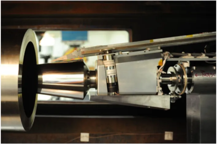
Figure 2. Cone model installed in SLDT. Diffuser cap-ture not installed for this image.
A three-axis model-integrated traverse was used to provide probe movement in the wall-normal (pitch of the probe head), downstream (parallel to the cone surface), and azimuthal directions. The traverse system is remotely controlled to provide the three-axis motion. The traverse rack is aligned to the cone surface (see Fig. 2 for a picture of the cone model installed in the tunnel). The leading edge of the traverse arm—just downstream of the probe at-tachment location—is preloaded with a teflon foot that slides on the cone surface. This mitigates un-wanted vibrations under aerodynamic loading when the arm is cantilevered forward. The s-axis motion along the cone surface is provided by a rack and pinion system and is driven by a miniature stepper motor. The travel extent along the cone for this test is 120 ≤ s ≤ 300 mm. The s-axis resolution is 0.081 mm, based on laser-tracker measurements
used to evaluate the accuracy of this motion.19 The azimuthal motion is achieved using a spur gear
configu-ration, where the larger gear is fixed on the model sting and the smaller gear rotates with the counter-balanced block located just downstream of the cone base. This motion is also driven by a miniature stepper motor. The total range of motion in the azimuthal-axis direction is−125◦≤φ≤125◦. An encoder provides position feedback and is mounted to the model sting. The encoder accuracy is estimated to be ∼0.1◦. The wall-normal motion is achieved by pivoting the probe head about a pivot point that is driven by a lead screw and miniature stepper motor. The relative rotational motion of the probe head is measured with a differential variable reluctance transducer (DVRT) displacement sensor. A calibration procedure was performed for each probe head that relates the translational motion of the DVRT displacement sensor to the relative locations of the probe-tip (see Kegeriseet al.16 for details on the calibration procedure). The range of travel for the wall-normal motion from the model surface is y ≈4 mm. The y-axis probe positions are capable of being set to within±6.5 µm for the boundary-layer surveys.19
B. Probes and Instrumentation
Cone surface pressures and temperatures were monitored and measured throughout the test campaign. The ten static surface pressures were measured with 34.5 kPa differential transducers utilizing an electronic pressure scanning system with a stated accuracy of 0.03 % full scale. The reference pressure was acquired with a 13.33 kPa absolute gage that has a stated accuracy of 0.05 % reading. The six surface temperatures were acquired using a thermocouple measurement card with integrated signal conditioning. The stated accuracy of the system for the type-K thermocouples used is 0.36◦C.
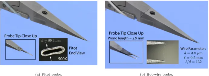
Mean pitot-pressure data were acquired in the cone boundary layer using a wedge-shaped pitot probe that was mounted on the three-axis model-integrated traverse system. A photograph of an example probe
500X
Probe Tip Close Up
Pitot End View
h= 89.4µm
(a) Pitot probe.
Probe Tip Close Up
Prong length = 2.9 mm Wire Parameters = 0.5 mm /d= 132 d= 3.8µm (b) Hot-wire probe.
Figure 3. Photographs of the boundary-layer probes and relevant dimensions: (a) Pitot probe and (b) hot-wire probe.
is shown in Fig. 3(a). For the pressure data, the pitot tube was flattened to have a frontal area with an approximate width and height of 285.03 µm and 89.42 µm (open area approximately 258.45×39.62 µm), respectively (see insets in Fig. 3(a)). The pitot probe was connected to an ultra-miniature pressure transducer using a 0.508-mm I.D. tubing. The small “dead” volume (1.485 mm3) of the pressure transducer and the
small volume of the tubing helped to minimize the settling time for the pitot probe. The typical stated accuracy of the transducer is 0.1 % full scale.
Mean total-temperature data were acquired with the wedge-shaped hot-wire probes (Fig. 3(b)) across the boundary layer. These are later referred to as cold-wire surveys in contrast to the traditional hot-wire surveys. For these measurements, the hot-wire probe cable was disconnected from the anemometer and connected to a precision 6.5-digit digital multimeter on a 100-Ω range for resistance measurements. The wire sensor resistance was then converted to total temperature (see discussion below in Section II.C).
Mean and unsteady mass-flux data were acquired with single-element hot-wire probes operated in a constant-temperature mode with a 1:1 bridge configuration. Two types of hot-wire anemometry measure-ments were acquired: 1) in the cone flow field to measure the boundary-layer flow field and 2) in the empty tunnel to obtain freestream mass-flux measurements. The former measurements were acquired using a wedge-shaped hot-wire probe, as shown in Fig. 3(b), that was mounted on the model-integrated traverse system. These boundary-layer hot-wire measurements represent the bulk of the reported data. The wire sensors used for the boundary-layer measurements were 3.8-µm platinum-plated tungsten wires with lengths ofl= 0.5 or 1 mm. Typical response bandwidths of the boundary-layer hot wires were estimated based on the traditionally-accepted square-wave-injection response to be in excess of 310 and 290 kHz for the 0.5 and 1-mm long wires, respectively. Details of the wedge-shaped probe body design for the pressure and hot-wire probes and the associated CFD analysis used to minimize the boundary-layer flow interference are provided by Owenset al.19, 24 The AC-coupled hot-wire output of the boundary-layer probe from the anemometer
was conditioned with a low-noise amplifier/filter before being digitized with a 16-bit A/D (analog-to-digital) converter at a rate of 1 MHz and a total of 2×10⁶ sample points. Programmable gain was applied by the
amplifier/filter system to maximize the dynamic range of the A/D. The signal was high-pass filtered with a 4-pole, 4-zero filter at 1 kHz (to reduce the vibrational response associated with the model-integrated traverse system) and anti-alias filtered with a 6-pole, 6-zero filter at 400 kHz. Additionally, hot-wire mea-surements were acquired in the tunnel freestream with an empty test section using the tunnel traverse. The hot-wire probes for these measurements were standard straight single-wire probes and had sensor diameters and lengths ofd= 5µm andl= 1.25 mm, respectively. The sensing elements here were also platinum-plated tungsten wires. The response bandwidths for the freestream probes typically exceeded 220 kHz. As with the boundary-layer anemometer signal, the AC-coupled output for the freestream probe was also conditioned with a low-noise amplifier/filter system before being digitized with the 16-bit A/D converter at 0.5 MHz and a total of 1×10⁶sample points. Programmable pre- and post-gain were applied by the amplifier/filter system
with an 8-pole, 8-zero filter at 200 kHz. For all hot-wire measurements, the anemometer was operated at high overheat ratios,τ = 0.8 or 0.9, so that the wires were sensitive primarily to mass flux, ρu. The mean hot-wire data were DC coupled and low-pass filtered at approximately 100 Hz before being acquired by a precision 6.5-digit digital multimeter on a 10-V range for voltage measurements.
An electronic fouling circuit was designed to indicate when the probe first makes contact to the model surface. Before each profile measurement (pitot or hot wire), the probe was electrically fouled on the model surface to set the y-axis location. This was achieved by slowly moving the probe (a few steps at a time) towards the wall until the pitot tip for the pitot probe and the prongs for the hot-wire probe made contact to the model surface. The probe was then retracted so that the probe became just unfouled with the surface. Using the DVRT calibration data referenced earlier and the position offset data (distance from the model surface to the center of the sensor location when fouled), they-axis locations were estimated. More details on this process are given by Kegerise, Owens, and King.16
C. Data Reduction
Mach number boundary-layer profiles were obtained from the pitot-pressure measurements. The average value of the ten static surface pressures on the cone surface was used as an estimate of the edge static pressure. This pressure agreed well with the Taylor-Maccoll conical-flow solution for a 7◦ half-angle cone. Using both the measured pitot pressure and the average surface pressure, we solved for the Mach number by applying the isentropic relations in the subsonic regime and the Rayleigh pitot tube formula in the supersonic regions.
The hot-wire reduction analysis was limited toM >1.2, where the Nusselt number becomes independent of Mach number. We followed the approach used by Smitset al.25by operating the wires at large overheats,
τ, so that the wire responded primarily to mass flux. The calibration equation was reduced to the form: E2
o=A+B·(ρu)
n, (1)
where A, B, and n are the calibration constants that were obtained from a least-squares curve fit. Hot-wire calibrations were conducted in SLDT either on the nozzle centerline with an empty test section or downstream of the conical shock with the model installed. The calibrations were performed at a nominally fixed total temperature,Tc, corresponding to our test conditions (Tc≈299.8±0.6 K).
A temperature correction to the anemometer bridge output was necessary to account for variations in T0(y) relative to Tc across the boundary layer, hence we applied a temperature correction
p
T0/Tc to the output bridge voltageEo. The relevant hot-wire equation to apply across the boundary layer now becomes
E2
o·(T0/Tc) =A+B·(ρu)n. (2)
Examples demonstrating the validity of this approach were presented in an earlier paper.16 In order to
estimateT0(y) across the boundary layer, a cold-wire survey was always acquired with each hot-wire survey.
For the cold-wire survey, the sensor resistance was measured at each wall-normal location. With the wire sensor submerged in the flow stream, the wire temperature equilibrates to the recovery temperature Tr (= ηrT0), where T0 is the local total temperature. The wire recovery factorηr has been shown to depend on both the wire Reynolds number,ρud/µ0, and Mach number. For supersonic Mach numbers, the recovery
factor is independent of Mach number.26, 27 The recovery factor is generally independent of the wire Reynolds
number forρud/µ0>20.28, 29 However, for the current test, values of the wire Reynolds number less than
20 were realized in the lower region of the boundary layer. The cold-wire calibrations were performed over the same mass-flux range as the hot-wire calibrations for each probe. The cold-wire calibration entailed measuring the wire sensor recovery resistancerr and the tunnel total temperatureT0 (nominally constant).
The wire recovery temperatureTrwas estimated using a linear resistance-temperature relationship, namely Tr= 1 α· rr−rref rref −Tref. (3)
Here, α (=0.0036 K−1) is the temperature coefficient of resistance and r
ref and Tref are the reference resistance and temperature near ambient conditions, respectively. The recovery factor was then estimated usingηr=Tr/T0, which is a function of the wire Reynolds number.
The subsequent mass-flux data reduction in the boundary layer is an iterative process since we do not know theηrin advance. We begin by making an initial guess forηr to computeT0. Equation 2 is evaluated
using the measured mean bridge voltage Eo and T0 to get the mean mass flux ρu. An updated value of
ηr is evaluated from the cold-wire calibration using the most recent value of ρu andT0 to update the wire
Reynolds number. This process is continued until a satisfactory convergence of bothρu andT0 is achieved
with the most recent values. This iterative process is done for all the boundary-layer measurement stations. The mean and unsteady bridge voltages are then combined to give the instantaneous value,Eo=Eo+Eo0. Now thatT0(y) is known across the boundary layer, the instantaneous mass fluxρuis obtained using Eq. 2
for each measurement station. The instantaneous mass flux is then decomposed into its mean and unsteady components, ρu =ρu+ (ρu)0. All power spectral densities, G
ρu, were estimated using the Welch Method. Each sample record was divided into 400 equal segments. Fifty percent overlapping was used and a Hanning data window applied to each data block. The frequency resolution for allGρu presented is 200 Hz.
Narrowband rms mass flux with bandwidths of ∆fbw= 5 kHz were computed to estimate the measured disturbance mode shapes and disturbance amplification growth rates within selected frequency bins. These rms mass-flux values are identified by the center frequency that is given by fc = 5,10,15, ...,100 kHz, and the energy is integrated over a frequency band offc−∆fbw/2 ≤f < fc+ ∆fbw/2. The mass-flux mode shapes at a givensstation are theh(ρu)0ivalues at the desiredf
c. The boundary-layer disturbance growth at a desiredfc is obtained by selecting the maximum mode-shape value atfcfor eachslocation. A curve fit for the maximumh(ρu)0iversusscan be computed for each value off
c, i.e., twenty curve fits for twenty fc values. We then denote the curve-fit functions as ˜Afc(s) such that an estimate of the growth rate is given as
−αi= 1 ˜ Afc dA˜fc ds . (4)
Two curve-fit models were used in this analysis. For the case with sparse s-measurement locations (noisy-flow conditions), an exponential function raised to the power of a second-order polynomial was selected as the functional form of ˜Afc(s). This provides for three curve-fit constants that were obtained by minimizing the square of the residuals. For the data with closely spacedsstations (quiet-flow conditions), a smoothing spline function30 was selected with all data points having the same weights. Goodness-of-fit metrics (e.g.,
summed square of residuals, correlation of determination, and rms error) were evaluated for both types of curve-fit functions and were found to be acceptable.
III.
Computations
The computations were performed over a 7◦ half-angle cone at the nominal test conditions of the exper-iment. The two-dimensional unsteady compressible Navier-Stokes equations in conservation form are solved in the computational curvilinear coordinate system. The viscosity is computed using Sutherland’s law and the coefficient of conductivity is written in terms of the Prandtl number. The governing equations are solved using a fifth-order accurate weighted essentially non-oscillatory (WENO) scheme for space discretization and a third-order, total-variation-diminishing (TVD) Runge-Kutta scheme for time integration.
The outer boundary of the computational domain lies outside the shock and follows a parabola. This ensures that the boundary-layer growth is accurately captured. At the outflow boundary, an extrapolation boundary condition is used. At the wall, viscous no-slip conditions are used for the velocity boundary conditions. The wall temperature condition is prescribed as a constant adiabatic temperature (268.2 K) near the nose tip (s < 51 mm) and is gradually followed by a linear wall temperature distribution that increases to Tw = 278.9 K at s = 300 mm. This wall temperature distribution is employed based on measurements of the six surface temperatures after the model is thermally conditioned.19 The density at the
wall is computed from the continuity equation. In the mean-flow computations, the freestream values at the outer boundary are prescribed. The steady mean flow is computed by performing unsteady computations using a variable time step until the maximum residual reaches a small value (∼10−11). A CFL number of 0.2
is used. Details of the algorithm solution and computational approach are given by Balakumaret al.31, 32, 33 Spatial stability analyses were performed on the computed mean-flow states at different streamwise locations. For this paper, the analysis is limited to parallel linear stability theory (LST) computations and focused on oblique first-mode instabilities. The form of disturbances used to perform the stability computations is given by
q(y, s, φ, t) = ˜q(y)e−αi·ei(αrs+mφ−2πf t) (5) whereqis the disturbed flow variable,αris the streamwise wavenumber, andmis the azimuthal wavenumber (integral number of azimuthal waves around the cone circumference). Analysis details of the LST
computa-tions are given by Balakumar.33, 34 Mean-flow and LST results are compared to experimental results in the
following section.
IV.
Results
The results to follow will be discussed for a few test conditions. All data were acquired with a nominal freestream Mach number of M∞ = 3.5 and nominal total temperature ofT0= 299.8 K. To aid the reader,
the test (or total-pressure) conditions are tabulated in Table 1. Our discussions will mostly reference con-ditions with respect to P0 and s, so this table will help facilitate the reader to navigate quickly between
(P0, s) variables and (Re∞, Ree, R) variables. One bleed-valves-closed, noisy-flow condition was tested at P0= 241.3 kPa to evaluate our approach as we expected to obtain excellent SNR (signal-to-noise ratio) of the
unsteady hot-wire measurements for these conditions. However, our main goal was to acquire measurements in the natural low-noise environment of the tunnel, knowing that we would have signal levels at least an order of magnitude smaller than those for the noisy case, resulting in reduced SNR.
We know from experience in low-speed work that receptivity and stability experiments are very sensitive to the state of the mean flow and environmental conditions. As a result, we exercised extreme care to carefully document the mean flow and environmental conditions to avoid ambiguous results as reported by Nishioka and Morkovin35 and Saric.36 We attempted to follow those guidelines in our supersonic stability
study. We first present results on the freestream and boundary-layer edge conditions downstream of the shock to evaluate our environmental conditions. Then, the mean flow is documented and compared with the computational results to establish the baseline flow conditions. Finally, we examine the measured stability characteristics and reconcile with the LST results.
A. Freestream and Boundary-Layer Edge Measurements
Before installing the model, freestream hot-wire measurements were acquired along the nozzle centerline to assess the low-noise performance of the re-polished Mach-3.5 axisymmetric nozzle. Data were acquired over a range of total pressures to evaluate the extent of laminar flow on the nozzle walls. We were able to achieve laminar flow just beyondP0= 448.2 kPa, which was less than the value ofP0= 630 kPa reported 25 years
ago.21 However, we did improve the low-noise performance of the pre-polished nozzle, which was limited to
P0≈241.3 kPa.
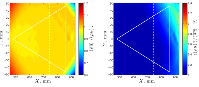
One future goal in our prediction toolkit is to be able to predict transition location reliably with an amplitude-based method. To that end, knowledge of the amplitude and spectral content of the incoming unsteady disturbances are essential. Consequently, an attempt was made here to document the freestream and boundary-layer edge unsteady flow field. First, hot-wire data were acquired along a vertical centerline plane in an empty test section to include 450.85≤X ≤927.10 mm and −50.8≤Y ≤50.8 mm in 6.35 mm increments in both directions. Mass-flux results forP0= 172.4 kPa are shown in Fig. 4 in the form of contour
plots. The plots also include lines that delineate the cone model (solid line) if it was present, and the nozzle exit location (dash line). The measured mean mass flux normalized by the freestream mass flux is presented in Fig. 4(a). The accompanying unsteady rms mass flux normalized by the measured mean mass flux is shown in Fig. 4(b). Parts of the upstream and downstream sections of the uniform-flow test rhombus are visible in
Table 1. Nominal freestream and edge Reynolds numbers for the test total-pressure conditions (M∞=3.5, T0=299.8 K). For the calculation of R in table, s is in units of mm.
P0, kPa Re∞×10−6, m−1 Ree×10−6, m−1 R Tunnel State 172.4 9.89 11.12 105.442×√s Quiet 241.3 13.85 15.57 124.761×√s Noisy 379.2 21.77 24.46 156.396×√s Quiet 448.2 25.73 28.91 170.021×√s Quiet
the mean-mass-flux contours, (ρu)/(ρu)∞. Meanwhile, the percent rms mass-flux contours clearly show that most of the cone resides in the quiet test core, i.e., where h(ρu)0i/(ρu)<0.1%. Fig. 4(b) also reveals that the nozzle-wall boundary-layer transition is not symmetric—boundary-layer transition on the upper nozzle wall precedes transition on the lower wall. Similar plots are presented in Fig. 5 forP0= 448.2 kPa (near the
maximum achievable quiet-flow conditions). The mean-mass-flux plots for both tunnel conditions are very uniform and consistent. The transition location on the nozzle wall moves forward for the higher pressure as expected. The asymmetry of the transition front is still apparent. This asymmetry was always present, even after successive cleaning attempts of the nozzle. Even at the highest tunnel pressure for quiet flow, it is important to note that more than 50% of the cone resided in the quiet test core (see Fig. 5(b)).
X
, mm
Y
,
m
m
500 600 700 800 900 −50 −40 −30 −20 −10 0 10 20 30 40 50(
ρ
u
)
/
(
ρ
u
)
∞ 0.6 0.7 0.8 0.9 1 1.1 1.2(a) Contour of normalized mean mass flux.
X
, mm
Y
,
m
m
500 600 700 800 900 −50 −40 −30 −20 −10 0 10 20 30 40 50h
(
ρ
u
)
0i
/
(
ρ
u
)
,
%
0 0.2 0.4 0.6 0.8 1 1.2 1.4(b) Contour of normalized percent rms mass flux. Figure 4. Contours of measured mass flux in the nozzle under quiet-flow conditions for P0≈172.4 kPa: (a)
normalized mean mass flux,(ρu)/(ρu)∞, and (b) percent normalized rms mass flux,h(ρu)0i/(ρu)%. The dotted and solid lines depict the nozzle-exit location and future location of the cone, respectively.
X
, mm
Y
,
m
m
500 600 700 800 900 −50 −40 −30 −20 −10 0 10 20 30 40 50(
ρ
u
)
/
(
ρ
u
)
∞ 0.6 0.7 0.8 0.9 1 1.1 1.2(a) Contour of normalized mean mass flux.
X
, mm
Y
,
m
m
500 600 700 800 900 −50 −40 −30 −20 −10 0 10 20 30 40 50h
(
ρ
u
)
0i
/
(
ρ
u
)
,
%
0 0.2 0.4 0.6 0.8 1 1.2 1.4(b) Contour of normalized percent rms mass flux. Figure 5. Contours of measured mass flux in the nozzle under quiet-flow conditions for P0≈448.2 kPa: (a)
normalized mean mass flux,(ρu)/(ρu)∞, and (b) percent normalized rms mass flux,h(ρu)0i/(ρu)%. The dotted and solid lines depict the nozzle-exit location and future location of the cone, respectively.
The normalized broadband rms mass flux for empty-tunnel freestream data are compared to boundary-layer edge data in Fig. 6. The rms mass fluxh(ρu)0iis integrated over a 100 kHz bandwidth. The boundary-layer edge data were acquired outside the boundary boundary-layer at y ≈ 2 mm along the s-axis direction and are shown as unfilled symbols. The empty-tunnel freestream data are extracted from the data shown in Figs. 4(b) and 5(b) based on the closeness in proximity of the (X, Y) location to the (s, y) location of the boundary-layer edge data. Both datasets are normalized byρu∞hence the slight difference in the normalized values (recall thatρuincreases across the shock). The values tend to collapse whenh(ρu)0iis normalized by the respective mean values, i.e.,ρu∞ orρue. For the data atP0 ≈175 kPa (Fig. 6(a)), the boundary-layer
edge data atφ= 0◦ show that the flow is quiet all the way to the last measurement station (s= 300 mm), unlike the empty-tunnel data, which begins to increase ats≈230 mm. We believe this discrepancy occurred due to a change in the nozzle quiet-flow performance—the nozzle was cleaned on multiple occasions (over a period of 5.5 months) between the empty-tunnel measurements and the subsequent boundary-layer edge measurements with the model. The noise level at φ =−90◦ for the boundary-layer edge data also shows an increase at a similar location as the empty-tunnel data. This trend in the boundary-layer edge data at φ=−90◦versus the values atφ= 0◦is also observed atP
0= 379.2 kPa (data not shown). Figure 6(b) shows
a similar plot for the largestRe∞condition. The first half of the cone is clearly in a quiet environment. The data in Fig. 6 demonstrate that the presence of the model and associated conical shock does not have an adverse effect on the h(ρu)0iamplitudes. Recall also that the empty-tunnel data and boundary-layer edge data were acquired with different probe bodies, wire sensor diameters and lengths, and traverse systems as discussed in Section II.B.
Next, we examine the spectral content of the data in Fig. 6. Figure 7 shows power spectral densities at three selected locations—one just upstream of the cone tip (empty-tunnel data only) and the other two at s≈125 and 250 mm, where both empty-tunnel data and boundary-layer edge data exist. For the data at P0 ≈ 175 kPa in Fig. 7(a), the solid lines show the empty-tunnel freestream data. Two features are
observed in the empty-tunnel spectra. First, there is an increase in the low-frequency energy in terms of amplitude and bandwidth as s increases, albeit small. The mechanism responsible for this increase is not clear, but this behavior has been observed in our two-dimensional quiet nozzle as well.16 Second, most of the
rms energy is dominated by thef-squared noise of the anemometer that starts at f ≈2 kHz for the most upstream location. The h(ρu)0i values presented previously are dominated by this f-squared noise when the flow is quiet. The dash lines in the figure represent the boundary-layer edge data (recall that these are high-passed filtered at 1 kHz and low-passed filtered at 400 kHz compared to the freestream data that are high-passed filtered at 0.25 Hz and low-passed filtered at 200 kHz). The spectra in Fig. 7(a) ats= 125 mm
0
100
200
300
0.0
0.2
0.4
0.6
0.8
1.0
h
(
ρ
u
)
0i
/
(
ρ
u
)
∞,
%
s
, mm
174.6,0 174.6,0 174.7,0 175.7,-90 P0( k Pa) ,φ(◦)(a) Normalized mass-flux fluctuations forP0≈175 kPa.
0
100
200
300
0.0
0.2
0.4
0.6
0.8
1.0
h
(
ρ
u
)
0i
/
(
ρ
u
)
∞,
%
s
, mm
452.0,0 450.6,0 450.8,0 451.3,-90 P0( k Pa) ,φ(◦)(b) Normalized mass-flux fluctuations forP0≈450 kPa. Figure 6. Normalized rms mass-flux fluctuation under quiet-flow conditions with (unfilled symbols) and without (filled symbols) the cone model in the test section: (a) P0≈175 kPa, and (b) P0≈450 kPa. The rms values
10
210
310
410
510
610
−1010
−910
−810
−710
−610
−510
−410
−3f
, Hz
G
ρ u(
f
)
(k
g
/
m
2/
s)
2/
H
z)
-3 125 253 125 250 s, mm(a) Power spectra atP0≈175 kPa.
10
210
310
410
510
610
−1010
−910
−810
−710
−610
−510
−410
−3f
, Hz
G
ρ u(
f
)
(k
g
/
m
2/
s)
2/
H
z)
-3 125 253 125 250 s, mm(b) Power spectra atP0≈450 kPa.
Figure 7. Measured freestream and boundary-layer edge power spectra under quiet-flow conditions for select s locations: (a) P0≈175 kPa, and (b) P0≈450 kPa. Solid lines represent empty-tunnel freestream spectra
and dash lines represent boundary-layer edge spectra.
have similar features except for greater spectral energy between approximately 2 to 20 kHz that is believed to be associated with the integrated-model traverse/probe system. A difference in the bandwidth of the low-frequency energy at s≈250 mm between the empty-tunnel and boundary-layer edge data is apparent and this difference is manifested in the observed increase ofh(ρu)0iin Fig. 6(a). Figure 7(b) shows a similar plot for the data atP0≈450 kPa. Similar features are observed here. The main difference being the agreement
between the empty-tunnel and boundary-layer edge spectra in the 2 to 20 kHz frequency band because the SNR is high.
B. Cone Base-Flow Measurements
The next step was to document carefully the mean-flow measurements and to compare the results with CFD results. The mean flow was acquired with both pitot-probe measurements and hot-wire measurements. 1. Boundary-Layer Pitot-Probe Measurements
With the cone model installed in the tunnel, we started the process of aligning the cone axis to the incoming flow. This process involved obtaining boundary-layer pressure profiles at various φ ands locations. After several iterations of adjusting the cone, we settled on what we considered to be an acceptable alignment. The Mach number profiles as derived from the measured pitot and surface pressures are shown in Fig. 8(a) for different values of φand s atP0 = 379.2 kPa. The experimental data are plotted in Blasius similarity
coordinates and are compared with the computed mean-flow profile ats= 302 mm. Recall that a self-similar solution was not assumed for our mean flow, but the actual mean-flow solution is approximately self similar for the measureds stations. There is excellent agreement between the experimental data and CFD results except for locations near the wall and fors= 125 mm. The excellent degree of cone alignment with respect to pitch and yaw is clearly demonstrated in the plot by the data collapse. Additional Mach number profiles over a range ofP0andsare presented in Fig. 8(b). Both plots in Fig. 8 indicate that there is a near similarity
with respect tosand φlocations andRe∞.
Preston tube measurements at the surface were also made to investigate the laminar-to-turbulent tran-sition state of the boundary layer. The pitot tube was traversed to a specified slocation and then moved down to foul the probe onto the model surface. Preston tube data were acquired at this position before the probe was retracted and moved to the next s location. Preston tube data were acquired for a range ofRe∞under quiet-flow conditions to include the maximum quiet-flow condition (Re∞= 25.81×10⁶ m−1
0
1
2
3
4
0
2
4
6
8
10
η
M
-0,125 -0,150 -0,200 -0,250 -0,275 -0,300 -90,150 90,150 -120,300 120,300 0,302 φ( de g) ,s( mm)(a) Mach number profiles for different φ and s locations at P0= 379.2 kPa.
0
1
2
3
4
0
2
4
6
8
10
η
M
P0( k Pa) ,s( mm) 175,301 381,300 451,200 451,250 451,300 379,302(b) Mach number profiles for various values of P0 and s at
φ= 0◦.
Figure 8. Measured Mach number profiles plotted in Blasius coordinates under quiet-flow conditions for: (a) differentφ and s locations, and (b) different P0 and s locations. The computed Mach number profile at
P0=379.2 kPa and s=302 mm is denoted by ‘ ’ .
or P0 = 448.2 kPa) and one noisy-flow condition (Re∞ = 13.92×10⁶ m−1 or P0 = 241.3 kPa). The unit
Reynolds number for the noisy-flow condition was selected so that the onset of transition was located in the accessible s range. Figure 9 shows the normalized Preston tube data for a range of test conditions and azimuthal locations. For the noisy-flow condition (filled symbols), boundary-layer transition onset, as demonstrated by the increase inPp/P0, begins atstr ≈192 mm. Meanwhile, for the quiet-flow condition, transition as measured by the mean-flow distortion is not realized; however, the data reported earlier by Chenet al.6 and King22 indicate that transition is imminent (note thatR2 = 8.7×10⁶ ats= 300 mm at
the maximum Re∞). Excellent azimuthal agreement is observed in the measured transition front for the noisy-flow condition in Fig. 9, which again demonstrates the degree of cone alignment and cone-tip sym-metry. The quiet-flow measurements also showed consistent results around the azimuth, i.e., no perceived transition onset.
2. Boundary-Layer Hot-Wire Measurements
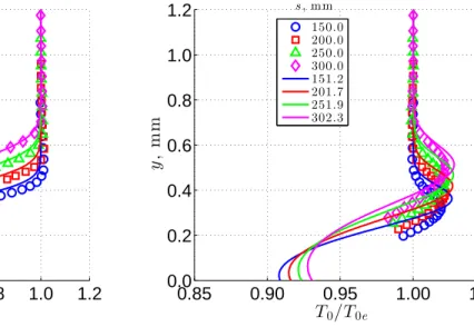
Hot-wire and cold-wire boundary-layer measurements were acquired along the cone for a range of tun-nel conditions. Reduced results in the form of mass flux and total temperature are shown in Fig. 10 for P0= 379.2 kPa. The measured profiles are plotted versus y for four slocations and are compared to the
respective CFD results. Very good agreement is observed for the normalized mass-flux profiles in Fig. 10(a), particularly for the downstream profiles. The normalized temperature profiles are shown in Fig. 10(b). Good agreement is observed for the temperature profiles, but the temperature peaks are slightly overpredicted by the CFD results. These plots and findings are representative of the other test conditions.
C. Unsteady Boundary-Layer and Stability Measurements 1. Measurements in Noisy Flow
Unsteady boundary-layer measurements are first presented for the noisy-flow condition atP0= 242.3 kPa.
The boundary layer transitioned from laminar to turbulent flow near the midsection of the cone. Mass-flux boundary-layer profiles were acquired at five streamwise locations along the cone surface froms= 125 to 225 mm. The maximum broadband rms mass flux at each s location is presented in Fig. 11(a). This maximum inh(ρu)0ioccurs near η≈4.2 to 4.6. The saturation location,s≈200 mm, in the figure gives an indication of transition onset as measured from the unsteady data. This agrees to within our measurement
100
150
200
250
300
0.020
0.025
0.030
0.035
0.040
0.045
0.050
P
p/
P
0s
(mm)
st r
φ(◦) ,P 0( k Pa) 0,175.4 0,312.4 0,417.4 0,449.3 -90,449.2 91,449.1 0,242.8 -90,242.3 91,241.2 0,241.4Figure 9. Normalized Preston tube data (Pp/P0) versus s. Filled symbols are for noisy-flow conditions and
unfilled symbols are for quiet-flow conditions.
0.0
0.2
0.4
0.6
0.8
1.0
1.2
0.0
0.2
0.4
0.6
0.8
1.0
1.2
(ρ
u
)
/
(ρ
u
)
ey
,
m
m
150.0 200.0 250.0 300.0 151.2 201.7 251.9 302.3 s, mm(a) Mean-mass-flux profiles for a range ofslocations.
0.85
0.90
0.95
1.00
1.05
0.0
0.2
0.4
0.6
0.8
1.0
1.2
T
0/T
0ey
,
m
m
150.0 200.0 250.0 300.0 151.2 201.7 251.9 302.3 s, mm(b) Total-temperature profiles for a range ofslocations. Figure 10. Measured boundary-layer profiles in quiet flow forφ=0◦and P0=379.2 kPa: (a) normalized mean
ρu, and (b) normalized T0. The computed mean profiles are denoted by lines.
resolution of swith the value (str ≈192 mm) obtained from the near-wall mean-flow distortion shown in Fig. 9. The correspondingN factor at transition from LST isN ≈3.9 forstr≈192 mm. Saturation occurs when h(ρu)0i/(ρu)
e ≈ 17% ats ≈ 200 mm. The corresponding power spectral densities at the maximum
h(ρu)0i are given in Fig. 11(b). Significant spectral broadening beyond f ≈100 kHz is clearly evident at s > 175 mm. The plot also includes boundary-layer edge spectra for the s = 125, 150, and 175 mm at y≈1 mm (largest wall-normal location) in dashed lines. For locations ofs >175 mm, the peak lobe of the broadband rms mass-flux profile extends beyond the maximum measured y location. The boundary-layer edge spectra for the locations presented in the figure show very little change with increasings. The ratios of the maximum to the edge broadband rms mass flux ats= 125, 150, and 175 mm areh(ρu)0i/h(ρu)0
ei= 5.0, 6.6, and 13.4, respectively.
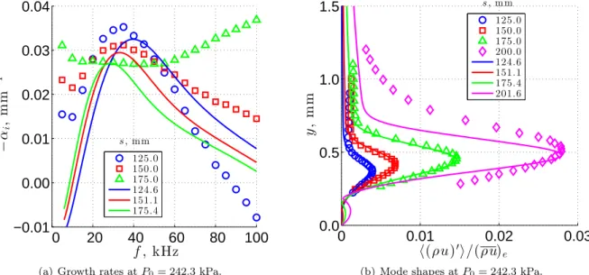
A plot of the growth rate versus frequency is presented in Fig. 12(a). The LST results are for an azimuthal wavenumber ofm= 20 (corresponding to the most unstable mode froms≈125 to 200 mm). The measured
−αi ats= 125 mm compare favorably with the LST growth rates. However, the comparison is very poor at s = 175 mm, particularly at the tails of the curve, where spectral broadening due to nonlinear effects are evident. Some degree of nonlinearity at the higher frequencies is believed to be present at s= 150 mm as well. The experimental maximum growth rates (in the vicinity of f ≈35 kHz) follow the same trend as the predicted LST results, i.e., decreasing maximum growth rate with increasings. The measured mode shapes at four measurement stations are presented in Fig. 12(b) forfc= 50 kHz. The LST eigenfunctions for f = 50 kHz andm= 20 are scaled to match the measured peak value for each profile. Excellent agreement is evident for all the profiles except fors= 200 mm, where the flow was highly nonlinear and the broadband disturbances began to saturate. Good-to-excellent agreement is realized for both the growth rates and mode shapes when the disturbances are small enough to preclude nonlinear effects.
100
0
150
200
250
5
10
15
20
h
(
ρ
u
)
0i
/
(
ρ
u
)
e%
s
, mm
(a) Amplitude growth atP0= 242.3 kPa.
10
210
310
410
510
610
−910
−710
−510
−310
−1f
, Hz
G
ρ u(
f
)
(k
g
/
m
2/
s)
2/
H
z)
125 150 175 200 225 s, mm(b) Power spectra atP0= 242.3 kPa.
Figure 11. Measured hot-wire data in noisy flow for φ=0◦ and P0=242.2 kPa: (a) maximum normalized
broadband rms mass flux, and (b) power spectral density at maximum broadband y locations. Boundary-layer edge spectra at y≈1 mm for the first three s stations are included in plot as dash lines.
0
20
40
60
80
100
−0.01
0.00
0.01
0.02
0.03
0.04
−
α
i,
m
m
− 1f
, kHz
125.0 150.0 175.0 124.6 151.1 175.4 s, mm(a) Growth rates atP0= 242.3 kPa.
0
0.01
0.02
0.03
0.0
0.5
1.0
1.5
h
(ρ
u
)
0i
/
(ρ
u
)
ey
,
m
m
125.0 150.0 175.0 200.0 124.6 151.1 175.4 201.6 s, mm(b) Mode shapes atP0= 242.3 kPa.
Figure 12. Reduced hot-wire data in noisy flow compared with linear stability theory for m = 20 at P0=242.2 kPa: (a) dimensional growth rates obtained from mass-flux growth, and (b) mode shapes at
2. Measurements in Quiet Flow
Next, we consider the unsteady boundary-layer measurements under quiet-flow conditions for P0 = 172.4,
379.2, and 448.2 kPa. At a total pressure ofP0= 172.4 kPa, no measurable instability above the electronic
noise floor was discerned along the entire length of the cone (data not shown). Matlis et al.14, 37 made
similar observations under quiet-flow conditions in the Mach 3.5 two-dimensional nozzle of the SLDT. Their measurements were acquired at a unit Reynolds number of 9.45×10⁶m−1(P
0= 172 kPa andT0= 311 K).
For the purpose of this report, no further results are provided at this test condition. For that reason, we tested at the two higher total pressures. At total pressures of Po = 379.2 and 448.2 kPa, the results were found to be qualitatively similar to one another, except that the broadband rms mass fluxes ats= 300 mm areh(ρu)0i/(ρu)
e≈3.5 and 6.4%, respectively. For that reason, both test conditions are discussed together. A plot of the maximum growth amplitude at selected frequency bins versus s location is shown in Fig. 13(a) forP0= 448.2 kPa. The even values offc(10, 20, ..., 100) are not shown for clarity. The broadband growth amplitude is also included in the figure. In general, the rms amplitudes decrease with increasing fc at a givens location. The most-amplified first-mode instabilities predicted for 250< s <300 mm by LST occur atf = 50 to 60 kHz andm= 30. The largest values of h(ρu)0ithroughout the measurement range do not coincide with the predicted most-amplified first-mode disturbances. To explore this further, we focused on two measured frequency bins: 1) a low-frequency bin (fc = 10 kHz) with substantial amplitude and 2) a frequency bin (fc = 50 kHz) within the LST-predicted most-amplified mode. Figure 13(b) presents the data for the maximum boundary-layerh(ρu)0i and the edgeh(ρu)0
ei, which are shown as unfilled and filled symbols, respectively. Note that the data up tos≈175 mm forh(ρu)0
eiatfc= 50 kHz are at thef-squared noise floor of the anemometer. LST predictions in the form of eN for f = 10 and 50 kHz and azimuthal wavenumberm= 30 for both frequencies are also included in Fig. 13(b). The LST results are scaled to match the measured data ats= 300 mm. The agreement between the measuredh(ρu)0iandeN for 10 kHz is very good over the entire measurement range. This suggests that the rms mass flux at 10 kHz is predominately driven by linear instability growth and not by the downstream external boundary-layer edge forcingh(ρu)0
ei.
The measuredh(ρu)0iat 50 kHz compares reasonably well with the correspondingeN fors >225 mm. The mode shapes for P0 = 379.2 and 448.2 kPa are given in Fig. 14 along with the scaled LST
eigen-functions for f = 50 kHz and m = 30. The maximum values of the measured normalized mass flux are very small (O(10−3)), so the measured mode-shape profiles are relatively noisy. However, although the SNR
is small, the mode shapes are clearly measurable at the latter measurement stations. The marginal SNR
100
0
150
200
250
300
1
2
3
4
5
6
7
h
(
ρ
u
)
0i
/
(
ρ
u
)
e,
%
s
, mm
fc, k H z 5 15 25 35 45 55 65 75 85 95 0-100(a) Maximum mass-flux growth within the boundary layer at P0= 448.2 kPa.
100
150
200
250
300
350
10
−410
−310
−210
−1h
(
ρ
u
)
0i
/
(
ρ
u
)
es
, mm
10 50 10 ( LST ) 50 ( LST ) 10 ( e dge ) 50 ( e dge ) fc, k H z(b) Comparison of maximum mass-flux growth with LST at P0= 448.2 kPa. Edge mass flux denoted with filled symbols. Figure 13. Mass-flux growth under quiet-flow conditions at P0=448.2 kPa: (a) normalized growth at selected
fc for the maximum measured mass flux, and (b) growth compared with linear stability theory at two values
improvement in the mode shapes for P0 = 448.2 kPa (Fig. 14(b)) versus P0 = 379.2 kPa (Fig. 14(a)) is
evident. The y locations of the peaks are slightly underpredicted by the LST eigenfunctions. Next, the corresponding growth rates are presented in Fig. 15. The growth rates forP0= 379.2 kPa in Fig. 15(a) are
fairly noisy, again partly due to the low SNR. The extreme scatter at f = 25 kHz resulted from vibration of the integrated-traverse/probe system in that frequency bin. The growth rates atf ≈30 kHz are over-predicted by linear theory. A similar plot for P0 = 448.2 kPa is shown in Fig. 15(b). The measured −αi for the first two measurement stations are again well below the LST predictions. As the SNR improved for the two latter stations (s= 290 and 300 mm), the growth rates are more akin to the LST predictions. The predictions underestimate the growth rates, peak frequencies, and frequency band, but the general features are fairly similar.
0
1
2
3
x 10
−30.0
0.5
1.0
1.5
h
(ρ
u
)
0i
/
(ρ
u
)
ey
,
m
m
250.0 275.0 290.0 300.0 249.8 274.5 290.8 300.4 s, mm(a) Mode shapes atP0= 379.2 kPa.
0
0.005
0.01
0.0
0.5
1.0
1.5
h
(ρ
u
)
0i
/
(ρ
u
)
ey
,
m
m
250.0 275.0 290.0 300.0 250.0 274.9 289.8 300.9 s, mm(b) Mode shapes atP0= 448.2 kPa.
Figure 14. Measured mode shapes under quiet-flow conditions and scaled eigenfunctions from LST (fc=50 kHz,
m=30): (a) P0=379.2 kPa, and (b) P0=448.2 kPa.
0
20
40
60
80
100
−0.01
0.00
0.01
0.02
0.03
0.04
−
α
i,
m
m
− 1f
, kHz
250.0 275.0 290.0 300.0 249.8 274.5 290.8 300.4 s, mm(a) Growth rates atP0= 379.2 kPa.
0
20
40
60
80
100
−0.01
0.00
0.01
0.02
0.03
0.04
−
α
i,
m
m
− 1f
, kHz
250.0 275.0 290.0 300.0 250.0 274.9 289.8 300.9 s, mm(b) Growth rates atP0= 448.2 kPa.
Figure 15. Measured growth rates in quiet flow compared with linear stability theory (m = 30): (a) P0=379.2 kPa, and (b) P0=448.2 kPa.
10
210
310
410
510
610
−910
−710
−510
−310
−1f
, Hz
G
ρ u(
f
)
(k
g
/
m
2/
s)
2/
H
z)
150 200 250 300 250( LST ) 300( LST ) s, mm(a) Power spectra atP0= 379.2 kPa.
10
210
310
410
510
610
−910
−710
−510
−310
−1f
, Hz
G
ρ u(
f
)
(k
g
/
m
2/
s)
2/
H
z)
150 250 290 300 250( LST ) 290( LST ) 301( LST ) s, mm(b) Power spectra atP0= 448.2 kPa.
Figure 16. Measured power spectra at the maximum h(ρu)0i in quiet flow for select s locations: (a) P0=379.2 kPa, and (b) P0=448.2 kPa. LST results are shown for comparison.
Finally, we consider the power spectral densities at the maximum broadband mass flux at selected s locations. Figure 16(a) shows the measured power spectral densities at four streamwise locations for P0= 379.2 kPa. At the latter two measurement stations, a broad peak begins to emerge in the spectra for
s= 250 and 300 mm. The scaled power spectra foreN versus frequency of the most unstable first-mode dis-turbance are also plotted for the last twosstations. Excellent agreement with respect to frequency is observed between the measured spectra and the LST predictions. Similar results are presented forP0= 448.2 kPa in
Fig. 16(b). The emergence of the most unstable first-mode instabilities is evident in the last threesstations. As before, excellent agreement is evident between the measured and predicted results. A low-frequency band (∼20 kHz) is also evident in the last two measurement stations.
V.
Discussion
The challenge in measuring naturally-occurring first-mode instabilities under quiet-flow conditions in a Mach-3.5 stream was clearly evident throughout this test campaign. However, similar hot-wire measurements by Lachowiczet al.,38Blanchard,39Rufer,40and Hofferthet al.41have been acquired at Mach 6 under
quiet-flow conditions for naturally-occurring second-mode instabilities on cones. Their results not only clearly demonstrated the presence of second-mode instabilities and harmonics but demonstrated the dominance of these second-mode instabilities in the transition process. The most-amplified instabilities at hypersonic speeds are two-dimensional (2-D) second-mode waves (m = 0), but for supersonic Mach numbers, the most-amplified instabilities are three-dimensional (3-D) first-mode waves with large values of the azimuthal wavenumber (typicallym >10). This raises a few fundamental questions:
1. What is the nature (2-D versus 3-D) of the disturbances that are most dominant or relevant in the freestream of wind tunnels?
2. What is the relative efficiency of the receptivity process in generating the 2-D versus 3-D most-amplified instability waves?
3. How are the 3-D first-mode disturbances with large m generated near the leading-edge region of the cone, where the circumference gets vanishingly small?
4. Are the inherent difficulties of such measurements at moderate to high supersonic Mach numbers due to the significantly lower first-mode amplitudes realized at Mach 3.5 versus the much larger second-mode amplitudes at Mach 6 (refer to computations by Mack7)?
Most of these are vexing questions to resolve experimentally, due in part to the current state-of-the-art measurement capabilities, i.e., the inability to acquire temporally and spatially resolved measurements with noise floor levels 2 to 3 orders of magnitude lower than hot-wire anemometry. Under quiet-flow conditions, our measured signal amplitudes were extremely small and could be smaller than or on the same order of magnitude as the anemometer f-squared noise (O(10−5) to O(10−4)). Additionally, we know in general
that the total measured mass flux within the boundary layer included both the forced response due to the freestream/boundary-layer edge excitation and the instability (free) response predicted by stability theory. Mack7 has shown that the peak value of the forced response can be 5 – 20 times as large as the freestream
value without any instability amplification. When both the forced and instability responses were comparable, the measured mass-flux values were difficult to interpret. With our current measurements, we are unable to estimate the relative importance of the forced and eigenvalue responses, i.e., the relative magnitude and phase between the forced response and eigenvalue response are unknown. However, DNS (direct numerical simulations) computations in conjunction with carefully conducted experiments may help to resolve these questions/issues.
So why are our measured low-frequency disturbance amplitudes (e.g.,fc= 10 kHz) so dominant relative to disturbance amplitudes (e.g., fc = 50 kHz) within the predicted most-amplified first-mode frequencies (see Fig. 13(b))? Here, we consider only the data acquired at the highestRe∞(P0≈448.2 kPa). At 10 kHz,
LST predicts an amplification ofeN ∼4 from the branch I location (s≈155 mm) to the last measurement location (s = 300 mm). But at 50 kHz, LST predicts amplification of approximately 4.4×10³ from the
branch I location (s ≈ 45 mm) to s = 300 mm. The measured boundary-layer edge disturbances and maximum boundary-layer disturbances for 10 kHz at its branch I location are both within our measurement capability (see Figs. 7(b) and 16(b) for spectra at s = 125 and 150 mm, respectively). In contrast, the measured freestream and boundary-layer edge disturbances at 50 kHz near its branch I location are below the anemometer noise floor (see Fig. 7(b) for spectra at s=−3 and 125 mm). For that matter, boundary-layer edge spectra (data not shown) indicate that the energy at 50 kHz is below the anemometer noise floor for all locations upstream of s ≈ 180 mm, and this is borne out in Fig. 13(b). The measured maximum boundary-layer disturbances at 50 kHz at our most upstream locations= 125 mm indicate that our measured values were above the anemometer noise floor (see spectra ats= 150 mm in Fig.16(b)); however, we do not know the relative importance of the forced versus instability responses in the measured mass flux. Given the aforementioned information with respect to our measurement limitations, we conjecture the following scenario. We can assume that the freestream power-spectral component at 50 kHz is approximately 2 orders of magnitude less than the component at 10 kHz—based on the extrapolation of the precipitous spectral rolloff with frequency (see the spectrum ats =−3 mm in Fig. 7(b)). With that assumption, the freestream/edge spectral amplitude component at 50 kHz is O(10−5). If the receptivity coefficient at the
branch I location (s ≈ 45 mm) is O(100), then we would expect amplitude measurements based on an
amplification ofeN ∼4.4×10³ to beO(10−2) or spectral power ofO(10−4). Interestingly, this O(10−4) in
spectral power agrees with our measurements ats= 300 mm (see Fig.16(b)). So referring back to Fig. 13(b) whereh(ρu)0i/(ρu)
e∼ O(10−2) ats= 300 mm, we can speculate based on LST thath(ρu)0i/(ρu)e∼2×10−6 at branch I (s≈45 mm) in the boundary layer, i.e., below our measurement capability.
Our measurements suggested that the flow was not measurably receptive to the freestream/edge dis-turbances that impinged on the latter portion of the cone surface. This was shown by the fact that the measured mass flux followed the LST disturbance growth at 10 kHz throughout that impingement region (refer to Figure 13(b)). DNS computations by Balakumer34 predicted that the receptivity location is near
the nose region on a smooth cone surface. Chen, Malik, and Beckwith6 tested a 5◦ half-angle cone under quiet-flow conditions with the cone tip located at two streamwise locations (7.6 mm apart). They concluded that the cone boundary layer is much more sensitive to the wind-tunnel noise in the vicinity of branch I than farther downstream, since they measured lower transition Reynolds numbers at the lowerRe∞for the downstream cone location. However, the data show that for the higher Re∞ conditions, where the branch I location is expected to move upstream, the transition Reynolds numbers are consistent at both cone lo-cations. The DNS34 and experimental6 results support our finding here that the boundary-layer was not
measurably receptive to the impinging freestream noise on the latter portion of the cone, well downstream of branch I locations.
Excellent agreement for large SNR data was observed for the noisy-flow condition. For the noisy-flow data, the exponential growth of the instability response is expected to overwhelm the forced response; thus, the measured mode shape approximated the LST eigenfunction, provided that the instabilities are still