Development of Unsteady Pressure-Sensitive Paint
Application on NASA Space Launch System
Nettie H. Roozeboom*, Jessie Powell†, Jennifer K. Baerny*, David D. Murakami*, Christina L. Ngo*, Theodore J. Garbeff*, James C. Ross*, Ross Flach*
*NASA Ames Research Center Moffett Field, CA 94035 † NASA Johnson Space Center
Houston, TX 77058
The key measurement to acquire for understanding unsteady flow is surface pressure. Unsteady Pressure-Sensitive Paint (uPSP) is an emerging optical technique used in wind tunnel testing to measure fluctuating surface pressures. Recently, tests were conducted on NASA’s Space Launch System in NASA Ames Research Center’s Unitary Plan Wind Tunnel to determine the aeroacoustics environment and assist in developing the buffet forcing functions. Unsteady PSP data was collected during this test campaign. Steady state PSP data, infrared thermography, shadowgraph, accelerometer data, and dynamic pressure transducer data were also collected. In all 50 TB of data were collected during the three days of testing. During these three days of testing, a repeating transonic and supersonic alpha sweep condition was acquired. This paper presents these two wind tunnel conditions and examines how the temperature influences the PSP data. In the first large demonstration of uPSP in 2015 on an NESC-, AETC-sponsored wind tunnel test, lifetime PSP results highlighted the influence the model temperature had on the PSP data. A best practice of heat soaking the model before acquiring calibration images was followed during the test campaign presented in this paper. An infrared thermography camera and thermocouples were installed in the model to collect more details of the model surface temperature. Data processing schemes for uPSP are still in development but will be briefly presented here as well.
I.
Introduction
any important physical problems in aerosciences involve unsteady, separated flows. The ability to measure and compute these flows has been a persistent challenge. Unsteady aerodynamics leads to unsteady loads which ultimately decrease system performance and shortens the system lifetime.
Traditionally, unsteady pressure transducers have been the instrumentation of choice for investigating unsteady flow phenomena. With recent advances in high-speed cameras, high-powered energy sources, and faster response pressure-sensitive paint, the unsteady pressure-pressure-sensitive paint (uPSP) technique has become another tool to investigate this critical flow, enabling time resolved measurements of unsteady pressure fluctuations within a dense grid of spatial points on a wind tunnel model. For wind tunnel tests acquiring high frequency pressure environment data, the common practice is to install hundreds of unsteady pressure transducers. Often 200 – 300 transducers are used for integrating pressure fluctuations over a specified area. This practice becomes a large monetary and time expense for the customer. An average cost is approximately $2,000 per transducer. This includes the instrument, machining of the holes for the instrument, and machining of the model once the instrument screen is installed to create a smooth model surface. However, other costs include the calibration of each transducer, installation, and inspection after installation in the wind tunnel. Even with the high transducer count, the data collected is still sparse and coverage is insufficient to provide accurate integrated unsteady loads on a wind tunnel model.
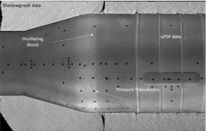
Results using only the pressure transducers provide overly conservative load predictions in some cases and underestimate load predictions in other areas depending on the flow characteristics1. Unsteady PSP has the ability to determine more accurate integrated unsteady loads but many research questions still remain open. The raw uPSP image and raw shadowgraph image show an oscillating shock on the model in Figure 1. The pressure transducers
M
locations noted by the black circles, indicate the flow phenomena is just downstream of the instrumentation. This is not surprising since the flow features change with the varying wind tunnel conditions and pressure transducers cannot be installed to capture every flow feature at every wind tunnel condition. Since uPSP is applied by a spray gun, it is continuously distributed. Also, if the model geometry can be painted, viewed from a camera, and excited by a lamp source, conceivably uPSP data can be collected. This is highly advantageous and very attractive when investigating unsteady aerodynamics.
Figure 1: Raw uPSP image with Raw Shadowgraph Image
A successful demonstration of the technology and software was performed in December 2017. The NASA goal is to mature the software from its current state to a stable test technology deployed at NASA Ames Research Center’s (ARC) Unitary Plan Wind Tunnel (UPWT) within the next year.
II.
Test Model and Wind Tunnel
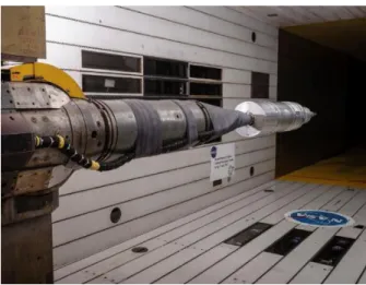
NASA’s Space Launch System (SLS) array of cargo and crew vehicle designs have been tested in many NASA facilities. This paper focuses on a recent NASA SLS Ascent Unsteady Aerodynamics Test (AUAT) performed at the NASA ARC UPWT 11-by 11-foot transonic test section2. The priority of this test was to acquire dynamic pressure environment to assist in determining the aeroacoustics environment and assist in developing the buffet forcing functions. In addition, a limited number of surface static pressures were installed. This test was also leveraged to demonstrate the current state-of-the-art of the NASA unsteady PSP systems. This demonstration was the most significant and most sophisticated implementation of the uPSP system technology to date. Figure 2 shows the SLS crew vehicle installed, painted with uPSP, and illuminated with PSP lights in the NASA ARC UPWT 11-by 11- foot transonic test section.
The 11-by 11-foot Transonic Wind Tunnel (TWT) lends itself nicely to optical measurement techniques with multiple windows on each wall of the tunnel, as shown in Figures 2 and 3. This wind tunnel has optical access on each of the four wall. On both side walls, there are 3 columns of 5 windows. On three rectangular windows in both the ceiling and floor, and several small porthole windows have been added to accommodate the frequent requests for optical test techniques, often acquired simultaneously.
Figure 2: SLS Crew Vehicle Painted with uPSP Figure 3: Optical Access at 11-by 11-foot TWT
III.
Instrumentation
A. Pressure-Sensitive Paint (uPSP)
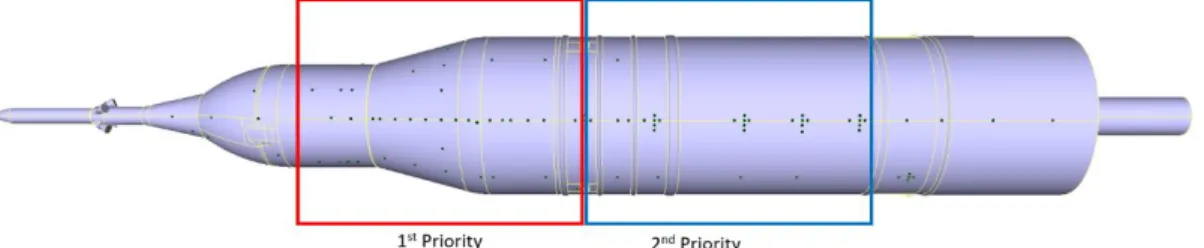
The porous, fast-response pressure-sensitive paint (FP-xxx) from Innovative Scientific Solutions, Inc (ISSI) was used for this test campaign because of the requirement to detect pressure fluctuations up to 20kHz. The paint’s pressure sensitive component is platinum (pentafluorophenyl) porphyrin (PtTFPP)3, 4 and the base is a polymer ceramic. Four Vision Research Inc. Phantom v2512, 12-bit, high-speed cameras (1280 x 800 pixels) with a quantum efficiency of ~50% at 650-nm were used to record the unsteady surface pressure data. One high-speed camera was mounted on each wall perpendicular to the flow and the high priority section of the model shown. The raw images from the uPSP cameras are also show in Figure 4 below. To optimize the limited number of cameras, the camera locations were installed to obtain quality data on the high priority sections of the model, shown in Figure 5. This camera placement did now allow for images of the Launch Abort Tower of the SLS vehicle to be acquired during this uPSP demonstration.
Once the uPSP portion of the test began, an epoxy base coat, the polymer-ceramic fast-response PSP base coat, and active PSP layer were applied. To reduce any damage to the pressure transducers, an adhesive dot was applied over the top of the instrument screen. Once the masks were removed after painting, the circular contrast between bare metal and PSP would be used as image registration targets. The small circular black dots in Figure 4, raw images, and Figure 5, computer model, indicate pressure transducer locations.
Figure 5: Regions of Interest for uPSP Data Collection
Lifetime PSP acquisition was also acquired during the unsteady PSP portion of the test. The lifetime system has eight CoolSNAP K4 12-bit cameras (2048 x 2048 pixels) evenly distributed around the test section plenum5. Bandpass filters centered around 650-nm were installed on each of the uPSP and lifetime PSP cameras to only record the signal emitted from the paint.
Forty (400-nm wavelength) Light Emitting Diodes (LEDs) were installed around the test section. Each lamp produces 12-14W of power. These LED lamps are used for paint excitation during both uPSP data collection and lifetime PSP data collection. Due to the differing acquisition methods, lifetime PSP and uPSP systems acquired data in sequence. The LEDs were pulsed to allow for the two gate images required for lifetime PSP technique. The LEDs then illuminated the model continuously while the uPSP system acquired data. The uPSP data and dynamic pressure transducer data were acquired at the same time.
B. Pressure Transducers
The priority of this test was to acquire dynamic pressure environment to assist in determining the aeroacoustics environment and assist in developing the buffet forcing functions. Two hundred fifty dynamic pressure transducers were used to measure the unsteady aerodynamics. The pressure transducers provided were a combination of new units, units harvested from existing models, and units borrowed from other NASA facilities. Approximately half of the pressure transducers supplied were absolute (15 psia) and half were differential (15 psid and 5 psid). All the pressure transducers were recorded by the NASA ARC UPWT Dynamic Data System (DDS).
C. Static Pressure Taps
A total of 176 surface static pressures measured with Digital Temperature Correction (DTC) Electronically Scanned Pressure (ESP) modules were installed across the vehicle.
D. Thermography
A FLIR SC8200 series mid-wave (3-5 μm), research grade infrared (IR) camera was positioned to image of the SLS model during the uPSP portion of the test. The SC8200 series is a megapixel (1024x1024) mid-wave IR camera that is most commonly deployed at the NASA ARC UPWT6,7,8 for infrared flow visualization purposes. The exposure time of an IR camera is dependent upon the radiance expected within the image field. Given the range of total temperature (typically 50-90 ⁰F) of the 11-by-11 foot facility, exposure times for the SC8200 series camera are on the order of 6 milliseconds.
E. Thermocouples
Six type J thermocouples were installed at a constant model phi along the length of the model. They are installed beneath but near the model surface. These were solely installed for collecting model surface temperature data during the uPSP portion of the test.
F. Accelerometers
A total of six tri-axis accelerometers were used. A single tri-axis accelerometer was mounted in the nose of the wind tunnel model. An additional tri-axis accelerometer was installed on the top of each camera. One accelerometer was installed on the floor of the ceiling hatch.
IV.
uPSP Processing Development
At a high level the uPSP processing approach follows these steps:1. Adjust the measured camera calibrations for the first frame in the video using the visible model targets, in this case the dynamic pressure transducers. Since the camera calibrations were computed from wind-off images, this adjustment captures sting deflection for each wind-on condition.
2. Develop a projection matrix for each camera using ray tracing and adjust the matrices for camera overlap. In overlap regions the weights of the cameras are determined by the angle between the camera and the model normal.
3. For each frame after the first, register the image to the first frame 4. Project the frame onto the model.
5. Convert image intensity to pressure.
There are two major goals of this development work. The first is to develop a suite of tools for processing and post-processing that are open source and general enough to be deployed to other wind tunnels. Other open source libraries, particularly OpenCV9and HDF510, have been highly leveraged to get these processing tools to their current level of functionality in a relatively short period of time. The second goal is to streamline the processing to dramatically reduce the time between gathering the data and looking at final results. For NASA ARC UPWT will be done by quickly moving the data from the wind tunnel to the NASA Advanced Supercomputing (NAS) facility, leveraging those parallel computing resources to reduce the data, then making the data available to researchers directly on NAS. This new pipeline addresses bottlenecks in data transfer and allows for much larger computing resources than could reasonably be deployed directly to the wind tunnel.
V.
Results
The variety and amount of data collected during this test is unprecedented. This section is a glimpse of the work conducted so far in regards to the uPSP demonstration. However, development of the processing software, development of tools to visualize the results, and evaluation of the data is still a work in progress.
To fully examine the uPSP data, the steady-state PSP data, dynamic pressure transducer data, static pressure transducer data, wind tunnel data, accelerometer data, IR thermography data, thermocouple data, and shadowgraph data must be considered. Currently, the accelerometer data, IR thermography data, thermocouple data, and shadowgraph data are only used passively in assessment of the uPSP data.
The uPSP intensity data is converted to pressure using the method proposed by Arnold Engineering Development Complex (AEDC)11,12 and used on a previous demonstration of the NASA uPSP system13. The data intensity time history is processed using intensity ratio technique, Iref/I. The reference image is an average of all the images from a single data point.
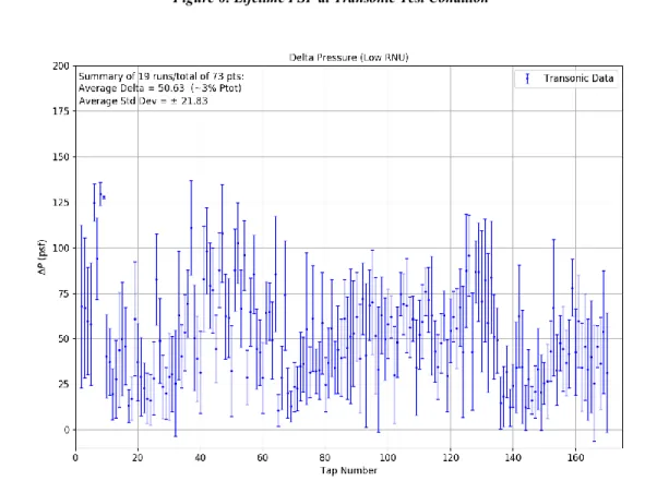
The lifetime PSP data was acquired and reduced using standard procedures for the method14,15. The lifetime PSP data was used to determine the gain, or calibration factor, for the uPSP data from intensity to pressure. Unlike the usual FIB pressure-sensitive paint used for the lifetime technique, the fast-response PSP has a strong sensitivity to temperature. This is evident in the steady-state PSP data, and comparisons to pressure tap data at the same location shows this sensitivity. Using a FIB pressure-sensitive paint, the lifetime PSP system is expected to have results with a margin of error of about 1% of the total pressure. Lifetime data analysis of the porous, fast response PSP had results with a margin of error between 3-5% of the total pressure. Figures 6 and 8 show lifetime PSP results for a transonic point and supersonic point, respectively, at alpha and beta equal to 0, and Figures 7 and 8 show the absolute value of the delta pressure computed from the pressure tap at a given location to lifetime PSP comparison at that same location. It is important to note, the data presented in the tap to PSP comparison plots below are for a repeat alpha sweep at constant beta angle equal to 0. In the pressure tap to PSP comparison plots the y-axis is in pounds per square foot (psf) and the x-axis is increasing order of taps identification (1-170). Generally, the taps are installed from vehicle nose to vehicle tail, and the characteristics of the curve show some dependence on tap location, therefore on the flow characteristics.
Figure 6: Lifetime PSP at Transonic Test Condition
Figure 7: Tap vs PSP Comparison for Transonic Test Condition
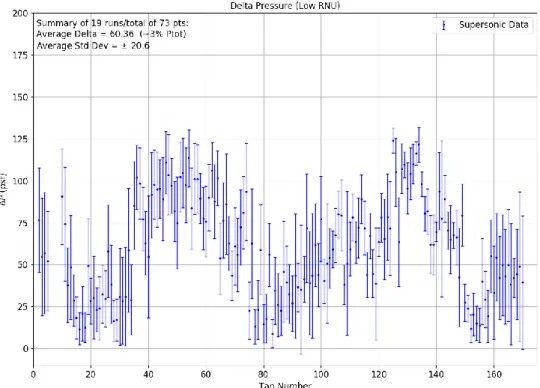
Figure 9: Tap vs PSP Comparison for Supersonic Test Condition
Given the high sensitivity the paint has to temperature, 6 thermocouples were installed in the model and an IR thermography camera was installed in the ceiling of the test section. Again, the thermocouples were installed just beneath the model surface, and the intention was to collect data to understand the temperature distribution on the model surface and compare to tunnel total temperature. All the temperature data presented below will all be in degrees Fahrenheit (°F).
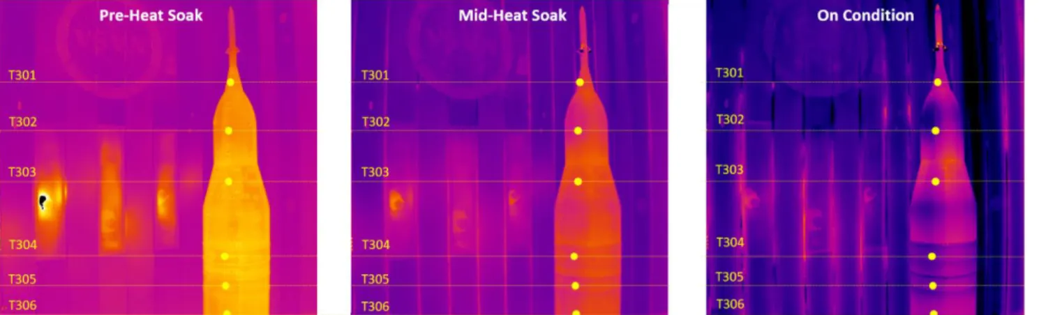
In 2015, the NASA Engineering and Safety Center (NESC) and NASA’s Aerosciences Evaluation and Test Capabilities (AETC) sponsored a wind-tunnel test at NASA ARC to investigate launch vehicle buffet using unsteady pressure-sensitive paint16. During this first demonstration of the uPSP technology in a production style wind tunnel environment, results showed the benefit of heat-soaking the model before acquiring calibration images for the PSP systems. The best practices learned during the buffet verification test were executed on this uPSP demonstration. To heat-soak the model, the wind tunnel was ran at conditions of high dynamic pressure to alter the temperature of the model closer to the temperature the model would be while on conditions for data collection. The plot to the side in Figure 10 shows the quantitative changes recorded by the thermocouples and the temperature distribution on the model before the wind tunnel is ran, while the wind tunnel is setting conditions, and when the wind tunnel is on condition for the heat-soak. The wind tunnel was ran approximately 20-minutes, and the thermocouple values were assess in real time to determine when the model surface temperature had reached a steady
state. The IR thermography images in Figure 11 show the relative temperature change on the model from the wind off condition to wind on condition. The approximate location of the thermocouples is shown in Figure 11 by a yellow
dot. Also, the identification name of each thermocouple is noted to the side, from T301 – T306. The exact temperature is not necessarily important, rather, it is more important to note the temperature differences before the heat-soak and while on condition and distribution of temperature. This procedure was repeated each morning before data collection.
Figure 11: Heat Soak IR Thermography Data After the model was heat-soaked for 20-minutes, the flow
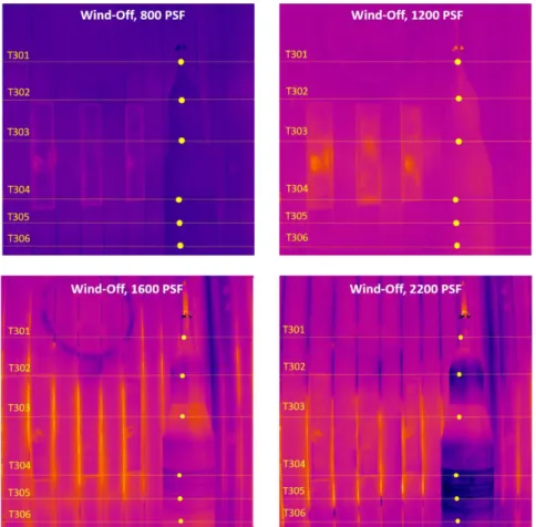
was turned off and the wind tunnel total pressure was adjusted for calibration images. For this test, the wind tunnel was pumped to 800 psf, 1200, psf, 1600 psf, and 2200 psf. This is usually referred to as ‘pump-down’ images. The tunnel pressure was held constant at each of these values and calibration data points were acquired with the lifetime PSP, uPSP, and IR thermography systems. In addition the thermocouple data, wind tunnel data, unsteady pressure transducer data, and pressure tap data were recorded at each point.
The lifetime PSP data processing involves several calibration steps14, 15. The first calibration applied is a laboratory calibration of the paint. AEDC’s laboratory calibration11in Figure 12 depicts the paint’s high temperature sensitivity. The reference temperature and pressure for this calibration was 70°F and 2000 psf, respectively. The next calibration applied to lifetime PSP data are the ‘pump-down’ calibration data. This in situ calibration addressed non-uniformities in the paint application and light distribution. As shown in Figure 13, the tunnel total temperature, in °F, (TTF) varies over 15°F from 800 psf to 2200 psf. The temperature variance over the model is fairly uniform, as shown in the IR thermography images in Figure 14, and thermocouples relatively small variation of approximate 1°F for each static pressure. The data shown in Figure 14 was collected after running the wind tunnel and collecting uPSP data for a full day.
As expected, the temperature will vary across the model while on condition, but the temperature fluctuation while on condition will be minimal.
Figure 12: AEDC Polymer-Ceramaic PSP Static Calibration
Figure 13: Thermocouple Data for 'Pump-Down' Calibration Data Points
Figure 14: IR Thermography Data for 'Pump-Down' Calibration Data Points
Rather than investigating these plots separately, it would be advantageous to view the lifetime PSP data and temperature data side by side. As mentioned above, the lifetime PSP data had an error 3-5 times what is usually expected. This is completely a function of the paint. The polymer ceramic PSP used was selected because of the requirement for a PSP with a high-frequency response. With this faster response, there is also a high temperature sensitivity. For the data presented in Figures 15 – 17, a single transonic point at alpha, beta equal to 0, 0 is presented. For the data presented in Figures 18 – 20, a single supersonic point at alpha, beta equal to 0, 0 is presented.
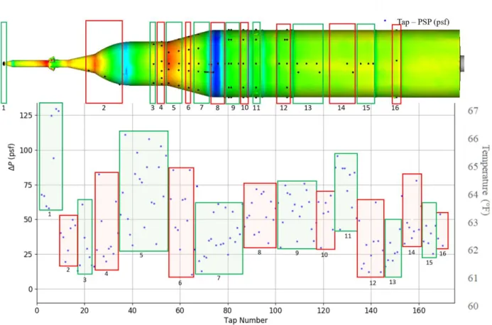
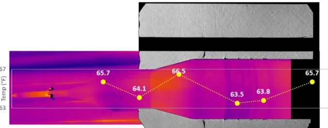
In Figure 15, the lifetime PSP data is shown above a plot where each marker indicates the absolute value of the tap value minus the PSP value at the tap in psf. As mention above, the taps are generally installed from vehicle nose to vehicle tail and plotted in order of identification number. To extract how the flow features are affecting the PSP, the taps in the same relative area were grouped together and numbered. For example, the first taps were located on the nose and had very high absolute delta pressure (|ΔP|), which would be expected with PSP data on the nose of small vehicle and also poor lighting on the nose. However, examining the next group of taps, group 2, the |ΔP| values are much smaller.This would also be expected since the view and lighting on this portion of the model was better and has relatively stable temperature and assumed to be closer to the surface temperature of the model when calibration images were collected. Looking further downstream at group 5 on the model, there is a large scatter of pressure comparison data. It can be seen in the lifetime PSP data that this is a region of high pressure and also high temperature, denoted by thermocouple T303, relative to surrounding thermocouples and IR thermography data shown in Figure 17. As the flow travels downstream, there is an area of low pressure. To further examine this low pressure, the shadowgraph data is consulted in Figure 16 and confirms the presence of a shock wave.
Figure 16 combines the lifetime PSP data, the thermocouple data, and raw shadowgraph data for the transonic condition. The thermocouple data is horizontally placed in the location of the actual temperature sensor hardware and vertically plotted on a scale from 63°F to 67°F with the exact temperature of each thermocouple denoted by its respective marker. The temperature recorded by the six thermocouples is also noted in the figure by the thermocouple marker. The raw shadowgraph data shows the shock wave presence at the area of low pressure in the lifetime PSP
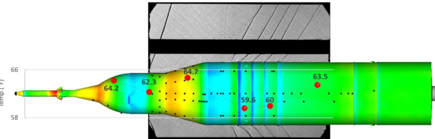
data. It is also show the model surface temperature decreases downstream of the shock wave as expected. Lastly, the qualitative IR thermography data is shown in Figure 17 along with the thermocouple data and raw shadowgraph data. The thermocouple marker again is place in the relative location horizontally the temperature sensor hardware is located. This figure again shows the flow features captured by the lifetime PSP data. There is an increase in temperature with adverse pressure gradient as the model diameter increases at the frustum. After the shock, the temperature decreases, and there are areas of low pressure just upstream of the flange rings on the rocket, which also creates perturbation in the flow as show in the shadowgraph still image.
The temperature variation is depicted in the thermography and thermocouple data, but the temperature sensitivity is depicted in the lifetime PSP data. Though the exact temperature values of the IR thermography images may be challenging to extract, the qualitative data provides a better insight to the surface temperature variation and the lifetime PSP data.
Figure 15: Lifetime PSP Data and Tap VS PSP Data for Transonic Test Condition
Figure 17: IR Thermograph Data, Thermocouple Data, and Shadowgraph Data for Transonic Test Condition
Figures 18 – 20 show the same plots but for a supersonic point at an alpha, beta equal to 0, 0. Figure 18 presents the lifetime PSP data, and the taps have been group together again in same fashion as presented previously. The lifetime PSP data shows an area of low pressure downstream of group 2. The indication of a shock wave can be seen barely in Figure 19 at the far left (upstream) edge of the shadowgraph still images. As the pressure increases at the frustum, the temperature increases as well, and high |ΔP| values are indicated in groups 5 and 6. Groups 8 and 9 see a large area of low pressure, followed by a shock, indicated by shadowgraph in Figure 20, with following shock waves created by the change in model geometry at the flange rings, again, and indicated by the shadowgraph still image. It is important to note, it is not necessarily high temperatures that produce a high difference between the pressure tap data and the lifetime PSP data, but rather this indicates a temperature difference from when the calibration images were acquired.
Figure19: Lifetime PSP Data, Thermocouple Data, and Shadowgraph Data for Supersonic Test Condition
Figure 20: IR Thermograph Data, Thermocouple Data, and Shadowgraph Data for Supersonic Test Condition
The temperature variation does not have an effect on the frequency content of the uPSP data, rather, since the lifetime PSP data is used for intensity to pressure conversion, the hypothesis is the temperature will have a scaling effect since the static pressure distribution will have error due to temperature. The temperature variation at a given grid node will be seen as a 5-10 Hz signal and can be easily filtered out of the uPSP data.
To convert the uPSP data to pressure, the methods referenced above were employed. However, this time history was moved to the frequency domain and compared to the dynamic pressure transduces, there was an offset between the two measurements. However, a second method to convert uPSP intensity data to pressure has been documented17 and uses the dynamic pressure transducers to calibrate the paint by equating the root-mean-square of the coefficient of pressure (CpRMS) in the time domain and then computing the Fourier transform.
In Figures 21 and 22 below, the pressure transducer data (blue) is compared to uPSP data (red) for the same 5 dynamic pressure transducers. Figures 21 and 22 show pressure sound density (PSD) of selected dynamic pressure transducers on the frustum section of the model and illustrate some common situations. In each figure the top row of PSDs show data processed using a steady-state PSP reference and a-priori paint gain calibrations, while in the bottom row the uPSP data has also been scaled to match the CpRMS of the transducers. In general the uPSP amplitudes are lower than the transducers amplitudes, although not always. To the right, a heat map of CpRMS gain is shown in the vicinity of the transducers. The red dots show the transducers locations.
Figure 21 shows measurements from a transonic run. KA906 shows good agreement after scaling, while K414 is limited by the noise floor at the highest frequencies. The effect of noise floor is more evident in K420, where uPSP does not track the dips shown in the transducer data. The signal in K412 is barely above the noise floor but the broad test section wall slot tone peak is visible through the noise, however, in this case the RMS scaling factor is actually less than one and pull the uPSP peak below the transducer peak. KA797 illustrates the case where scaling and
considering the noise floor are not sufficient. There are low frequency components present in the uPSP data that are not present in the transducer data. Since the images are registered, model motion and camera motion can be dismissed. The calibration factor heat map shows that over much of this area, the gain factors are close to or below unity. Figure 22 shows the same information, but for a supersonic condition. Overall, the agreement between uPSP and transducers tends to be better in the quieter supersonic regime. The calibration factor heat map appears very different from the transonic case, and are generally around 2. This will be a function of the flow phenomena present. For the transonic, the transducers shown are downstream of the shock wave mentioned above in Figures 15-17. There is temperature fluctuation approximately 3°F in this small section of the model. However, for the supersonic condition, the leading shock is much further forward. This would suggest when a strong dynamic pressure fluctuation or signal is present, the uPSP data captures more of the energy than when it is weaker
Figure 21: Transducer and uPSP PSD Comparisons for Selected Transducers at a Transonic Test Condition
Figure 22: Transducer and uPSP PSD Comparisons for Selected Transducers at a Supersonic Test Condition
VI.
Future Work
The research and development currently under way is focused on developing the processing software and assessing the quality of the uPSP data. More research needs to be conducted examining how the dynamic pressure transducer data can benefit the uPSP results. The dynamic pressure transducers must be used for the verification and validation of the uPSP data. The overall goal is not to replace pressure transducer instrumentation, but rather optimize where the transducers are located. Often the whole model is not viewable, and it would be advantageous to install transducers where optical access is limited. Algorithms need to be developed on how to handle areas with poor visibility with patching of transducer data.
Also, the dynamic pressure transducers are sampled at very high rates with build-in anti-aliasing filters. The same does not exist for uPSP data. By examining the dynamic pressure transducer data past the uPSP Nyquist frequency, one can assess the effects of aliasing on the uPSP data.
Also, on the last day of the test campaign, several dynamic pressure transducers were compared to results before paint was applied to the model. Unsurprisingly, the paint did affect the transducer signal. After inspection of several transducers, there were a noticeable step around the transducer due to the presence of the adhesive dot applied to protect the transducer hardware. After removal of the adhesive dot, a step remained around the transducer, and this step affected the data collected. The area around several transducers was sanded down before data collection on the last day. This data needs to be assess closer. Much attention was given to optimizing the painting process and the data collection process to not negatively affect the test productivity, however, the painting process and the process to protect the transducers from paint should be reevaluated, and also any sanding that may need to be conducted should be considered. Figures 23 and 24 show a single transducer’s physical appearance before and after sanding. A noticeable step surrounds the transducer where the adhesive dot was removed after painting. Once the surface around the transducer was sanded, the paint quality was degraded. However, this affect has not been quantified.
Figure 23: Transducer K952 Before Sanding Treatment Figure 24: Transducer K952 After Sanding Treatment
The NASA ARC UPWT facility tones are well documented and attenuating these tones in the dynamic pressure transducer data is typically conducted by customers of the wind tunnel. The same attenuation of the blade passing frequency, the model support tones, and the test section wall slot tones needs be applied to the uPSP data.
More development work is currently being conducted to produce plots like above in FIG to quickly assess the uPSP data quality compared to dynamic pressure transducer data. The frequency comparison plots above are a quick way to assess the value of the uPSP data, however, the more desired deliverable is to integrate the uPSP data using the same method the transducers are processed to calculate integrated loads.
This paper has shown the use of two calibration methods to compute pressure data at each grid node and compute frequency spectra with uPSP data. This process needs to further assess and understood. This is the first time two calibration methods have been applied to a data set. It is evident with this data set that the calibration method proposed by AEDC is not sufficient as the only calibration to be applied to the data. A worthy activity would be assess the data quality only using the dynamic pressure transducers to calibrate the uPSP data.
The effects of temperature on the lifetime PSP data needs to be further investigated. As for the heat-soaking, it would be advantageous to quantify the benefit this activity has on the lifetime PSP data.
The hardware and implementation in the wind tunnel is well-understood, however, it is evident the lighting is insufficient and has a direct effect on the quality of the data. Adding more lights specifically on the front and aft end of the mode would be helpful.
Currently, the accelerometer data has not been included. Though the images are registered, there should not be any indication of model or camera motion. However, it still would be advantageous when assess how well the image registration routine worked to know what model motion frequency and camera motion frequency was present.
To continue maturing the system past pressure-time histories, open discussion and collaboration with customers of the uPSP data is being conducted. The final data product to be delivered by the uPSP team is not pressure-time
histories, but rather the final data products needed by the customer. Along with the data products will be tools to aid in the process of comprehending the uPSP data set.
VII.
Acknowledgments
The authors would like to thank the NASA Aeronautics Evaluations and Test Capabilities (AETC) (formally the NASA Aeronautics Test Program (ATP)) for the support and funding of the PSP equipment and continuing the investment of new, state-of-the-art technology, like unsteady PSP. The authors would also like to thank the Space Launch System (SLS) Program for their investment and willingness to demonstrate the unsteady PSP technology. Resource supporting this work were provided by the NASA High-End Computing (HEC) Program through the NASA Advanced Supercomputing (NAS) Division at NASA Ames Research Center. Lastly, Ms. Roozeboom would like to thank Mr. Matt Krakenberg for your continued dedication to the team and careful installation of the uPSP equipment.
VIII.
References
1Sekula, M. K., Piatak, D. J., Rausch, R. D., Ross, J. C., and Sellers, M. E., “Assessment of Launch Vehicle Buffet Forcing Functions Developed Using Unsteady Pressure Sensitive Paint”, 56th AIAA Aerospace Sciences Meeting, AIAA SciTech Forum, San Diego, CA, January 2019.
2Amaya, M. A., and Boone, A. R., “Calibration of the 11- by 11-Foot Transonic Wind Tunnel at the NASA Ames Research Center,” AIAA 2005-4277. AIAA 41st AIAA/ASME/SAE/ASEE Joint Propulsion Conference and Exhibit, Tucson, Arizona, July 2005.
3Flaherty, W., Reedy, T. M., Elliot, G. S., Austin, J. M., Schmit, R. F., and Crafton, J., “Investigation of Cavity Flow Using Fast-Response Pressure Sensitive Paint.” AIAA 2013-0678, 51st AIAA Aerospace Sciences Meeting, Grapevine, TX, January 2013.
4Gregory, J. W., Asai, K., Kameda, M., Liu, T., and Sullivan, J. P. “A Review of Pressure-Sensitive Paint for High Speed and Unsteady Aerodynamics.” Proceedings of the Institution of Mechanical Engineers, Part G, Journal of Aerospace Engineering, Vol. 222, No. 2, pp. 249-290, (2008).
5Roozeboom, N.H., Baerny, J.K., “Guide for Pressure-Sensitive Paint Testing at NASA Ames Research Center Unitary Plan Wind Tunnel”, AIAA 2017-1055, 55th AIAA Aerospace Sciences Meeting, Grapevine, Texas, January 2017.
6Garbeff, T.J., et al, "Wind Tunnel Flow Field Visualizations of the Space Launch System Vehicle Ascent", 57th AIAA Aerospace Sciences Meeting, AIAA SciTech Forum, San Diego, CA, January 2019.
7Garbeff, T.J., Baerny, J.K., "A Qualitative Investigation of Selected Infrared Flow Visualization Image Processing Techniques", 57th AIAA Aerospace Sciences Meeting, AIAA SciTech Forum, San Diego, CA, January 2019.
8Garbeff, T.J., Baerny, J.K., “Recent Advancements in the Infrared Flow Visualization System for the NASA Ames Unitary Plan Wind Tunnels”, AIAA 2017-1051, 55th AIAA Aerospace Sciences Meeting, AIAA SciTech Forum, Grapevine, Texas, January 2017.
9Bradski, G. (2000). The OpenCV Library. Dr. Dobb’s Journal of Software Tools.
10The HDF Group. Hierarchical Data Format, version 5, 1997-2018. http://www.hdfgroup.org/HDF5/.
11Sellers, M.E., Nelson, M.A., Roozeboom, N.H., Burnside, N., “Evaluation of Unsteady Pressure Sensitive Paint
Measurement Technique for Space Launch Vehicle Buffet Determination, AIAA 2017-1402, 55th AIAA Aerospace Sciences Meeting, Grapevine, Texas, January 2017
12Sellers, M. E., Nelson, M., and Crafton, J.W., "Dynamic Pressure-Sensitive Paint Demonstration in AEDC Propulsion Wind Tunnel 16T", AIAA 2016-1146, 54th AIAA Aerospace Sciences Meeting, AIAA SciTech Forum, San Diego, CA, January 2016. 13Roozeboom, N. H., Ngo, C. L., Powell, J. M., Baerny, J. K., Murakami, D. D., Ross, J. C., and Murman, S., AIAA 2018-1031, 56th AIAA Aerospace Sciences Meeting, AIAA SciTech, Kissimmee, Florida, January 2018.
14Sellers, M. E. “Advances in AEDC’s Lifetime Pressure-Sensitive Paint Program.” AIAA Paper 2005-7638, U.S. Air Force T&E Days, Nashville, TN, December 2005. 7Sellers, M. E. “AEDC’s Portable Pressure-Sensitive Paint Data Acquisition System.” AIAA Paper 2007-1606, U.S. Air Force T&E Days, Destin, FL, February 2007.
15Sellers, M. E. “AEDC’s Portable Pressure-Sensitive Paint Data Acquisition System.” AIAA Paper 2007-1606, U.S. Air Force T&E Days, Destin, FL, February 2007.
16Schuster, D. M, et al, “Investigation of Unsteady Pressure-Sensitive Paint (uPSP) and a Dynamic Load Balance to Predict Launch Vehicle Buffet Environments,” NESC-RP-14-00962, November 2016.
17Panda, J., Roozeboom, N. H., and Ross, J. C., "Wavenumber-Frequency Spectra of Pressure Fluctuations on a Generic Space Vehicle Measured via Fast-Response Pressure-Sensitive Paint", AIAA 2017-1406, 55th AIAA Aerospace Sciences Meeting, AIAA SciTech Forum, Grapevine, Texas, January 2017.