Vortex Generators in a Streamline-Traced, External-Compression Supersonic Inlet

(1)

1

American Institute of Aeronautics and Astronautics

Vortex Generators in a Streamline-Traced, External-Compression Supersonic Inlet

Ezgihan Baydar*_{and Frank K. Lu}†

University of Texas at Arlington, Arlington, Texas 76019

and

John W. Slater‡ and Charles J. Trefny§

NASA Glenn Research Center, Cleveland, OH 44135

Vortex generators within a streamline-traced, external-compression supersonic inlet for Mach 1.66 were investigated to determine their ability to increase total pressure recovery and reduce total pressure distortion. The vortex generators studied were rectangular vanes arranged in counter-rotating and co-rotating arrays. The vane geometric factors of interest included height, length, spacing, angle-of-incidence, and positions upstream and downstream of the inlet terminal shock. The flow through the inlet was simulated numerically through the solution of the steady-state, Reynolds-averaged Navier-Stokes equations on multi-block, structured grids using the Wind-US flow solver. The vanes were simulated using a vortex generator model. The inlet performance was characterized by the inlet total pressure recovery and the radial and circumferential total pressure distortion indices at the engine face. Design of experiments and statistical analysis methods were applied to quantify the effect of the geometric factors of the vanes and search for optimal vane arrays. Co-rotating vane arrays with negative angles-of-incidence positioned on the supersonic diffuser were effective in sweeping low-momentum flow from the top toward the sides of the subsonic diffuser. This distributed the low-momentum flow more evenly about the circumference of the subsonic diffuser and reduced distortion. Co-rotating vane arrays with negative angles-of-incidence or counter-rotating vane arrays positioned downstream of the terminal shock were effective in mixing higher-momentum flow with lower-momentum flow to increase recovery and decrease distortion. A strategy of combining a co-rotating vane array on the supersonic diffuser with a counter-rotating vane array on the subsonic diffuser was effective in increasing recovery and reducing distortion.

Nomenclature

A = area

AIP = aerodynamic interface plane

hvg = height of a vortex generator Lvg = length of a vortex generator M = Mach number

Nvg = number of vortex generators p = pressure

svg = spanwise spacing between vortex generators T = temperature

VGs = vortex generators

x,y,z = Cartesian coordinates

xvg = streamwise location of the vortex generator array  = boundary-layer height

vg = angle-of-incidence of the vortex generator

*_{NASA Harriett G. Jenkins Fellow, Aerodynamics Research Center, Mechanical and Aerospace Engineering} Department, Box 19018, AIAA Student Member.

†_{Professor and Director, Aerodynamics Research Center, Mechanical and Aerospace Engineering Department, Box} 19018, AIAA Associate Fellow.

‡_{Aerospace Engineer, Inlets and Nozzles Branch, MS 5–12, 21000 Brookpark Road, AIAA Senior Member.} §_{Aerospace Engineer, Inlets and Nozzles Branch, MS 5–11, 21000 Brookpark Road, AIAA Senior Member.}

(2)

2

IDR = radial total pressure distortion

IDC = circumferential total pressure distortion

W = flow rate Subscripts

0 = freestream flow conditions

2 = AIP flow conditions

cap = reference capture condition

t = total or stagnation conditions

I. Introduction

Recent studies have examined streamline-traced, external-compression (STEX) supersonic inlets for turbine-powered aircraft flying at Mach 1.6.1–3_{A STEX inlet is characterized by an external supersonic diffuser obtained} from tracing streamlines through an axisymmetric, inward-turning parent flowfield containing a strong, oblique terminal shock. Section III will provide further details on the STEX inlet. Previous computations, have demonstrated that STEX inlets have about one-tenth of the inlet cowl wave drag and one-third of the external sound pressure disturbances compared to traditional axisymmetric and two-dimensional inlets.1_{The reduction of external sound} pressure disturbances could be correlated to the strength of sonic boom disturbances. These positive characteristics of STEX inlets are due to the low external cowl angle. However, the inlet total pressure recovery of the STEX inlet was about 3% lower than the traditional inlets. Further, the inlet total pressure distortion was higher for the STEX inlet and approached unacceptable values. This reduction of recovery and increase in distortion was due to the adverse effects of the terminal-shock/boundary-layer interaction, which created a low-momentum region within the subsonic diffuser.

One approach for reducing the low-momentum region is to use boundary-layer bleed in the vicinity of the terminal-shock/boundary-layer interaction. A porous bleed region downstream of the terminal shock has been shown through CFD simulations to increase the total pressure recovery and reduce distortion of the STEX inlet.3_{However, a bleed} system adds complexity and weight to the aircraft in the form of the required ducting and control of the bleed flow. Further, the loss in momentum of the bleed flow creates a drag component. For this work, it was decided to only consider a flow control approach using only passive devices that did not require external energy input or the injection or removal of flow.

The primary objective of this work was to explore the use of vortex generators (VGs) on the external supersonic diffuser and the subsonic diffuser to reduce the adverse effects of the terminal-shock/boundary-layer interaction. A previous study was conducted that involved a Mach 1.6 two-dimensional inlet with a normal-terminal-shock/boundary-layer interaction that created a two-dimensional low-momentum region in the subsonic diffuser.4 Rectangular vanes and ramps with triangular planforms were used to mix higher-momentum flow with the lower-momentum flow. The vanes or ramps were arranged as a linear array across the span of the inlet. Vanes were grouped as counter-rotating pairs with opposite angles-of-incidence. Each pair of vanes or ramps created a symmetric vortex with an upwash at the center. Symmetrical vortices were desired because the low-momentum region was two-dimensional. Locations upstream and downstream of the terminal-shock/boundary-layer interaction were explored. The main conclusion of that study was that vanes performed much better than ramps in reducing the low-momentum flow and radial distortion. The height of the vanes had the greatest effect with vane heights comparable to half of the boundary layer height being the most effective. Vanes positioned downstream of the terminal-shock/boundary-layer interaction were more effective than those positioned upstream of the interaction.

The STEX inlet created an asymmetric low-momentum region within the subsonic diffuser. One approach for reducing such asymmetry, and thereby reducing the total pressure distortion, is to use vanes arranged as a co-rotating array to redistribute the low-momentum region about the circumference of the subsonic diffuser. This approach was used successfully by Anderson et al. to reduce distortion for a subsonic diffuser with an S-bend.5_{The desired effect} of the co-rotating vane array was to sweep the boundary layer to redistribute the low-momentum flow.

The approach of the current work was to use rectangular vanes to either create vortices or sweep the boundary layer flow. The five geometric factors of the vanes explored in this work included the height, length, angle-of-incidence, circumferential spacing, and axial location. The vanes were arranged as arrays of counter-rotating vane pairs and co-rotating vanes with positive or negative angles-of-incidence. Also studied was the placement of the VGs upstream or downstream of the terminal shock/boundary-layer interaction.

The methods of design of experiments (DOE) and statistical analysis were used to explore the significance of the geometric factors of the vanes with respect to their ability for improving the total pressure recovery and distortion in the STEX inlet.6_{Fractional factorial studies were used to screen the five geometric factors to determine which were}

(3)

3

most significant. Two or three factors were then varied for response surface methodology (RSM) studies involving the building of quadratic models of the variations of the inlet performance measures with respect to the factors. These models were used to search for optimum vane arrays.

The flow through the STEX inlet and about the vortex generators was computed using methods of computational fluid dynamics (CFD) to solve the steady-state, Reynolds-Averaged Navier-Stokes (RANS) equations. Section II discusses the solution of the RANS equations as implemented into the Wind-US CFD flow solver.7_{The geometric} and computational modeling of the STEX inlet is discussed in Section III. The baseline flowfield through the inlet with no vortex generators is also discussed in that section. Section IV discusses further details on the vane vortex generators. Section V discusses the results of the studies of the STEX inlet with the vane vortex generators and the search for optimum vane arrays for the STEX inlet.

II. CFD Analysis Methods

Methods of computational fluid dynamics (CFD) were used to compute the turbulent flow through the STEX inlet. The Wind-US flow solver was used to solve the steady-state, Reynolds-Averaged Navier-Stokes (RANS) equations for flow properties on a multi-block, structured grid within the flow domain about the inlet.7_{The CFD solutions} allowed visualization of the flowfield to better understand the shock structures, boundary layers, and other flow features within and about the inlet. From the flowfield, the inlet performance measures were obtained.

A. Reynolds-Averaged Navier-Stoke Equations

With the presence of terminal shock/boundary-layer interactions in the inlet, fluctuations in density are significant. Density-weighted averaging of the Navier-Stokes equations are required for the current problem. The Favre-averaged Navier-Stokes equations takes instantaneous flow quantities, and replaces it with the sum of the mean 𝑢̃𝑖 and the fluctuating 𝑢_𝑖′′ parts:

𝑢𝑖= 𝑢̃𝑖+ 𝑢𝑖′′ (1)

where the Favre-averaged mean value at a fixed place in space is defined as

𝑢̃𝑖=_𝜌̅1 lim 𝛥𝑡→∞ 1 Δ𝑡∫ 𝜌𝑢𝑖𝑑𝑡 𝑡₀+𝛥𝑡 𝑡0 (2)

With the Favre-averaging procedure, the time-averaged mean velocity is 𝑢̃̅ = 𝑢̃_𝑖 _𝑖 and the time-averaged fluctuation velocity is 𝜌𝑢̅̅̅̅̅ = 0′′ . For the momentum equation, the additional term is the Reynolds stress 𝜌𝑢̅̅̅̅̅̅̅̅̅_𝑖′′𝑢_𝑗′′. For the energy equation, the additional terms are the Reynolds stress, the Reynolds heat flux 𝜌𝑢̅̅̅̅̅̅̅̅̅𝑗′′ℎ′′, molecular diffusion

𝑢𝑖′′𝜏𝑖𝑗

̅̅̅̅̅̅̅ and turbulent transport 𝜌𝑢̅̅̅̅̅̅̅̅̅̅̅̅_𝑖′′𝑢_𝑖′′𝑢_𝑗′′. The Favre-averaged Navier-Stokes equations can be written as

𝜕𝜌̅ 𝜕𝑡+ 𝜕𝜌̅𝑢̃𝑗 𝜕𝑥𝑗 = 0 (3) 𝜕𝜌̅𝑢̃𝑖 𝜕𝑡 + 𝜕 𝜕𝑥𝑗[𝜌̅𝑢̃𝑖𝑢̃𝑗+ 𝑃̅𝛿𝑖𝑗− (𝜏𝑖𝑗 𝐿 _{+ 𝜏} 𝑖𝑗𝑇)] = 0 (4) 𝜕 𝜕𝑡[𝜌̅ (𝑒̃ + 1 2𝑢̃𝑖𝑢̃𝑖+ 𝑘)] + 𝜕 𝜕𝑥𝑗[𝜌̅𝑢̃𝑗(ℎ̃ + 1 2𝑢̃𝑖𝑢̃𝑗+ 𝑘) − 𝑢̃𝑖(𝜏𝑖𝑗𝐿 + 𝜏𝑖𝑗𝑇) + (𝑞𝑗𝐿+ 𝑞𝑗𝑇)] = 0 (5) 𝑃̅ = 𝜌̅𝑅𝑇̃ (6) 𝜌̅ℎ̃ = 𝜌̅𝑒̃ + 𝑃̅ (7)

The superscript L denotes the laminar quantity while the superscript T denotes the turbulent quantity. The laminar and turbulent stresses are determined from

𝜏𝑖𝑗𝐿 = 𝜇𝐿( 𝜕𝑢̃𝑖 𝜕𝑥𝑗+ 𝜕𝑢̃𝑗 𝜕𝑥𝑖− 2 3 𝜕𝑢̃𝑘 𝜕𝑥𝑘𝛿𝑖𝑗) (8)

(4)

4

𝜏𝑖𝑗𝑇 = 𝜇𝑇( 𝜕𝑢̃𝑖 𝜕𝑥𝑗+ 𝜕𝑢̃𝑗 𝜕𝑥𝑖− 2 3 𝜕𝑢̃𝑘 𝜕𝑥𝑘𝛿𝑖𝑗) − 2 3𝜌̅𝑘𝛿𝑖𝑗 (9)

The laminar and turbulent heat fluxes are

𝑞𝑗𝐿= − 𝜇𝐿 𝑃𝑟𝐿 𝜕ℎ̃ 𝜕𝑥𝑗 (10) 𝑞𝑗𝑇= − 𝜇𝑇 𝑃𝑟𝑇 𝜕ℎ̃ 𝜕𝑥𝑗 (11)

The laminar viscosity is computed from Sutherland’s law

𝜇𝐿= 𝜇0( 𝑇 𝑇0) 3/2_𝑇 0+ 𝑆0 𝑇 + 𝑆0 (12)

where 𝜇0= 2.329x10−8 slug/ft − s, 𝑇0 = 518.67 𝑅, and 𝑆0 = 216.0 𝑅. The molecular and turbulent Prandtl numbers are 𝑃𝑟𝐿 = 0.72 and 𝑃𝑟𝑇 = 0.90.

B. Source Term Vortex Generator Model

A source term is added to the momentum (Eq. 4) and energy (Eq. 5) equations to simulate a lift force generated by a vane-type vortex generator. The source term modeling is known as the BAY model in Wind-US.8_{The BAY} model has been applied for vane-type vortex generators within subsonic and supersonic flows.8_{The BAY model does} not account for the viscous forces on the vanes, and so, the losses in total pressure due to the vanes are not modeled. The inputs to the BAY model include the grid range that would contain the vane, the angle-of-incidence of the vane, and the planform area of the vane. The BAY model imposes a lifting-force source term within the flow equation and aligns the local flow velocity with the vane incidence. The lifting force source term L is computed from

𝐿⃗ =𝑐1𝑆𝛼𝜌̅ 𝑢̃2𝑙̂ 𝑉𝑡𝑜𝑡

(13)

where u is the local velocity magnitude, _Vtot_{is the sum of the volumes of the cells where the force is applied,}α is the angle of incidence of the vane in respect to the primary flow, ρ is the local density, S is the vane planform area, 𝑙̂ is the unit vector in the direction of the lifting force acting on the flow, and 𝑐_{1 is an empirical constant. Bender et al.} calibrated 𝑐1 by examining the integrated cross-flow kinetic energy, √𝑘.9 For 𝑐1>5, √𝑘 approaches an asymptotic value because the model source term starts to dominate the other terms in the governing equations. The default value in the Wind-US solver is 𝑐1= 10. This term is added to both Favre-averaged momentum and energy equations:

𝜕𝜌̅𝑢̃𝑖 𝜕𝑡 + 𝜕 𝜕𝑥𝑗[𝜌̅𝑢̃𝑖𝑢̃𝑗+ 𝑃̅𝛿𝑖𝑗− (𝜏𝑖𝑗 𝐿 _{+ 𝜏} 𝑖𝑗𝑇)] = 𝐿𝑖 (14) 𝜕 𝜕𝑡[𝜌̅ (𝑒̃ + 1 2𝑢̃𝑖𝑢̃𝑖+ 𝑘)] + 𝜕 𝜕𝑥𝑗[𝜌̅𝑢̃𝑗(ℎ̃ + 1 2𝑢̃𝑖𝑢̃𝑗+ 𝑘) − 𝑢̃𝑖(𝜏𝑖𝑗𝐿 + 𝜏𝑖𝑗𝑇) + (𝑞𝑗𝐿+ 𝑞𝑗𝑇)] = 𝑢̃𝑖𝐿𝑖 (15) C. Turbulence Model

The shear-stress transport (SST) turbulence model devised by Menter10_{is based on the following equations.}

𝜇𝑇 = 𝑎1𝜌̅𝑘/max (𝑎1𝜔, Ω̃𝐹2) (16) 𝜕(𝜌̅𝑘) 𝜕𝑡 + 𝜕(𝜌̅𝑢̃𝑗𝑘) 𝜕𝑥𝑗 = 𝜕 𝜕𝑥𝑗[(𝜇𝐿+ 𝜎𝑘𝜇𝑇) 𝜕𝑘 𝜕𝑥𝑗] + 𝑃 − 𝛽 ∗_{𝜌̅𝜔𝑘} (17) 𝜕(𝜌̅𝑘) 𝜕𝑡 + 𝜕(𝜌̅𝑢̃𝑗𝑘) 𝜕𝑥𝑗 = 𝜕 𝜕𝑥𝑗[(𝜇𝐿+ 𝜎𝑘𝜇𝑇) 𝜕𝑘 𝜕𝑥𝑗] + 𝛾∗ 𝜈𝑇𝑃 − 𝛽𝜌̅𝜔 2_{+ (1 − 𝐹} 1)𝜎𝑑 𝜌̅ 𝜔 𝜕𝑘 𝜕𝑥𝑗 𝜕𝜔 𝜕𝑥𝑗 (18)

(5)

5

𝑃 = 𝜏𝑖𝑗𝑇 𝜕𝑢̃𝑖 𝜕𝑥𝑗= [𝜇𝐿( 𝜕𝑢̃𝑖 𝜕𝑥𝑗+ 𝜕𝑢̃𝑗 𝜕𝑥𝑖) − 2 3(𝜇𝑡 𝜕𝑢̃𝑘 𝜕𝑥𝑘− 𝜌̅𝑘) 𝛿𝑖𝑗] 𝜕𝑢̃𝑖 𝜕𝑥𝑗 (19)

𝐹1= tanh(𝑎𝑟𝑔14), 𝑎𝑟𝑔1= min (max(Γ1; Γ2) ; Γ3) (20)

𝐹2= tanh(𝑎𝑟𝑔22), 𝑎𝑟𝑔2= min (2Γ1; Γ2) (21) Γ1=_β√𝑘_∗_ωy (22) Γ2= 500𝜈𝐿 ωy2 (23) Γ3= 4𝜌̅𝜎𝑤2𝑘 y2_𝐶𝐷 𝑘𝑤 (24) 𝐶𝐷𝑘𝑤= max (𝜎𝑑 𝜌̅ 𝜔 𝜕𝑘 𝜕𝑥𝑗 𝜕𝜔 𝜕𝑥𝑗; 10 −20₎ (25)

The SST model is a two-layer model, where a 𝑘 − 𝜔 formulation is used near the wall and a 𝑘 − 𝜖 formulation is used in the outer part of the boundary layer and in free-shear regions. The 𝑘 − 𝜔 model is of particular interest since it is well-suited for adverse pressure gradients. Selection of the proper closure coefficients is controlled via the blending function 𝐹1. The constants in the SST model are calculated from the constants of the Standard Launder 𝑘 − 𝜖 and Wilcox 𝑘 − 𝜔 turbulence models. The term 𝐶𝐷𝑘𝑤 is the cross-diffusion term of the transformed dissipation equation of the Standard Launder 𝑘 − 𝜖 model.

D. Wind-US Flow Solver

The Wind-US flow solver uses a cell-vertex, finite-volume representation of the RANS equations for which the flow solution is located at the grid points.7_{The RANS equations are solved using an implicit time-marching algorithm} with a first-order, implicit Euler method using local time-stepping to converge the flow solution to the steady-state. The temperatures allowed the use of the calorically-perfect air model. The inviscid fluxes of the RANS equations are modeled using a second-order, upwind Roe flux-difference splitting method. The flow is assumed to be fully turbulent with the turbulent eddy viscosity calculated using the two-equation Menter shear-stress transport (SST) model.10

III. STEX Baseline Inlet

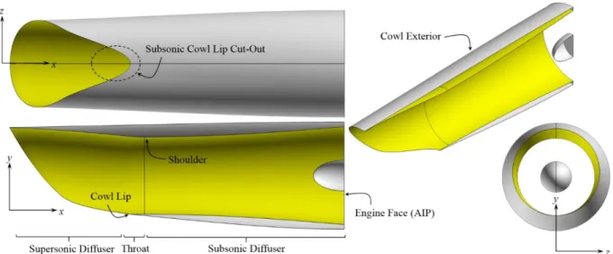
The streamline-traced, external-compression (STEX) inlet was designed for a future test in the NASA Glenn 8x6-foot supersonic wind tunnel. Figure 1 shows views of the STEX inlet. This section discusses the design of the STEX inlet, the computational flow domain, the boundary conditions for the computational simulations, the generation of the grid, and the baseline flowfield.

A. STEX Inlet Design

The flow conditions ahead of the inlet were a Mach number of M0 = 1.664, a total pressure of pt0 = 21.535 psi,

and total temperature of Tt0 = 622.5 oR. The engine face had a diameter of 0.979 ft with an axisymmetric spinner with

an elliptic profile. The ratio of the diameter of the spinner at the engine face to the diameter of the engine face was 0.315. The ratio of the length of the spinner to its diameter was 2.0. The engine corrected flow rate at the engine face corresponded to a mass-averaged Mach number of M2 = 0.478. The aerodynamic interface plane (AIP) was located

at the engine face. The design of the inlet and the generation of the geometry was performed using the SUPIN (Supersonic Inlet Design and Analysis) tool.11_{The axisymmetric parent flowfield for the STEX inlet was established} using the Otto-ICFA-Busemann method.2_{The internal angle of the leading edge was -5.0 degrees. The parent} flowfield contained a leading, weak oblique shock followed by an isentropic supersonic compression which ended with a strong oblique shock that decelerated the flow to Mach 0.9 and turned the flow into the axial direction. The surface of the external supersonic diffuser was created by tracing streamlines in the upstream direction through the parent flowfield starting from a circular tracing curve at the throat. The circular tracing curve was offset from the

(6)

6

axis-of-symmetry of the parent flowfield to result in a scarfed leading edge for the external supersonic diffuser. The throat section contained a rounded shoulder to aid the turning of the subsonic flow into the subsonic diffuser. The shoulder of the inlet indicates the start of the subsonic diffuser at x = 0.387 ft where the origin of the coordinate x = 0.0 ft is located at the origin of the axisymmetric parent flowfield. The throat also featured a “cut-out” at the bottom of the leading edge of the inlet. This “cut-out” allowed for greater subsonic spillage downstream of the terminal shock and the smooth positioning of the terminal shock with change in inlet flow rate.3_{The subsonic diffuser was created} to be axisymmetric about the inlet axis and with length of 2.0 ft that resulted in an equivalent conical angle of 2.94 degrees. The STEX inlet had a capture area of Acap = 0.597 ft2 and inlet length of Linlet = 3.353 ft. The reference

capture flow rate was computed using the freestream flow conditions and the capture area and had a value of Wcap =

0.9397 slugs/s. The inlet total pressure recovery computed by SUPIN was pt2/pt0 = 0.934.

Figure 1. The STEX inlet. B. Computational Flow Domain and Boundary Conditions

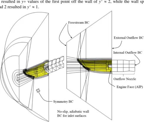
The CFD simulations required the generation of a computational flow domain about the inlet and the setting of boundary conditions. Figure 2 shows the flow domain and boundary conditions used for the CFD simulations of the STEX inlet. The inlet and the flow was symmetric about the plane at z = 0.0 ft, and so, the flow domain only included half of the inlet and flowfield. A symmetry boundary condition was applied at the plane z = 0.0 ft. The internal and external surfaces of the inlet formed a portion of the boundary of the flow domain where non-slip, adiabatic viscous wall boundary conditions were imposed. The flow domain had inflow boundaries upstream and about the inlet where freestream boundary conditions were imposed. The total pressure and temperature of the freestream state (p0,T0)

presented above corresponded to conditions of the NASA Glenn 8x6-foot wind tunnel. At the end of the cowl exterior, the domain had an outflow boundary where supersonic extrapolation boundary conditions were imposed. At the design operating condition of the inlet, the terminal shock sat at the axial position of the cowl lip. Downstream of the terminal shock, the internal flow was subsonic. Within the throat section, the subsonic flow was turned past the shoulder and further diffused in the subsonic diffuser as the flow approached the engine face. Downstream of the engine face, a converging-diverging outflow nozzle section was added to the flow domain to set the inlet flow rate. The throat of the outflow nozzle was set to be choked, and so, the inlet flow rate was varied by changing the cross-sectional area of the nozzle throat. Increasing the area of the nozzle throat also increases the engine-face corrected flow rate and decreases the “back-pressure” at the engine face. The outflow boundary of the nozzle was supersonic, which allowed a non-reflective extrapolation boundary condition to be imposed. This approach minimizes adverse effects of the internal outflow boundary condition on the flow at the engine face.

C. Computational Grid

Multi-block, structured grids were generated for the flow domain using SUPIN. SUPIN automatically established the number of grid points along the edges of the flow domain using inputs for the grid spacing of the first grid point normal to the wall (swall), grid spacing within the throat section in the streamwise direction (sx), and grid spacing in

the circumferential direction (sc). SUPIN then created the surface grids for the inlet and flow domain boundaries.

The volume grids for each block were then formed. SUPIN also created the boundary condition file for the Wind-US CFD flow solver. Grids were generated for a grid convergence study involving three levels of grid refinement. Table 1 lists the grid spacings used for the base grid and two levels of grid refinement. Also listed are the resulting number

(7)

7

of grid points within the inlet in the axial (Nx) and circumferential (Nc) directions for each grid. The wall grid spacing

for the base grid resulted in y+ values of the first point off the wall of y+_{2, while the wall spacing used for the}

refined grids 1 and 2 resulted in y+_1.

Figure 2. Flow domain and boundary conditions for the STEX inlet CFD simulations. D. Baseline Inlet Flowfield

The baseline inlet was the STEX inlet with no vortex generators. The paragraphs below describe the features of the flowfield for the baseline inlet and present the four inlet performance measures used to characterize the inlet: inlet flow ratio, inlet total pressure recovery, inlet circumferential distortion (IDC), and inlet radial distortion (IDR). The computational flowfield was initialized at all grid points with the flow conditions associated at the inflow to the inlet. The CFD simulations were performed until iterative convergence was obtained when the inlet performance measures had variations less than 0.10% of their mean values.

Figure 3 shows the Mach number contours on the symmetry plane (z = 0) of the baseline flowfield for three different inlet flow ratios. The oblique shock from the leading edge descends from left to right at a shock angle of -45 degrees and passes well ahead of the cowl lip. The Mach numbers decrease along the external supersonic diffuser in the streamwise direction. The terminal shock wraps around the cowl lip and intersects the top of the supersonic diffuser near the shoulder. Downstream of the terminal shock, the flow is subsonic and the Mach number decreases as the flow is diffused approaching the engine face.

The first measure of inlet performance was the inlet flow ratio (W2/Wcap), which was defined as the inlet flow rate

(W2) divided by the reference capture flow rate (Wcap). The inlet flow rate was the rate of flow passing through the

AIP and was computed as the mass-average of the flow through the outflow nozzle.

The second measure of inlet performance was the inlet total pressure recovery (pt2/pt0), which was defined as the

mass-averaged total pressure at the AIP (pt2) divided by the freestream total pressure (pt0). The mass-averaged total

pressure at the AIP was computed from the flowfield on the computational grid at the AIP.

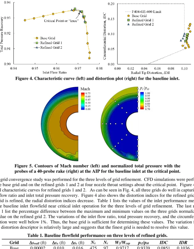
The variation of the inlet total pressure recovery with the inlet flow ratio is the inlet characteristic curve, which is also known as the “cane” curve because its resemblance to a walking cane. Figure 4 shows the characteristic curve for the baseline STEX inlet. The bend of the curve is the “knee”. The characteristic curve illustrates how the inlet operates with respect to inlet flow rate and total pressure recovery. The critical operating condition is when the inlet flow ratio is at its maximum with the maximum total pressure recovery. The STEX inlet was designed so that critical operating point would coincide with the design engine-face corrected flow rate in which the engine-face Mach number is M2 = 0.478. The characteristic curve of Fig. 4 identifies a solution point at the critical operation in which the inlet

flow ratio is W2/Wcap = 0.9710. The STEX inlet has some inherent spillage of 1.0 – 0.971 = 2.9%. The middle image

of Fig. 3 shows the baseline inlet flowfield near critical inlet operation. The terminal was positioned just upstream of the cowl lip. The top image of Fig. 3 shows the subcritical operation of the inlet. The terminal shock was pushed

(8)

8

forward of the cowl lip due to excess flow being spilled past the cowl lip downstream of the terminal shock. The inlet flow ratio is less than the critical operating value. The total pressure recovery decreases because the terminal shock is pushed forward on the external supersonic diffuser and into higher Mach number flow where normal shock total pressure losses are greater. Subcritical inlet operation involves engine-face corrected flow rates that are less than the value associated with the critical operating condition, which might be due to reduction of the throttle of a turbine engine. The supercritical operating conditions involve an increase in the engine-face corrected flow rate over the value associated with the critical operating condition, which might be due to an over-speed of a turbine engine. The inlet flow ratio is already at its maximum, and so, the total pressure recovery reduces. Supercritical operation is indicated by the segment of the characteristic curve that is the nearly vertical segment below the critical point or “knee”. The bottom image of Fig. 3 shows the inlet in supercritical operation. The terminal shock structure was altered as the top portion of the terminal shock separated from the lower portion and was drawn into the inlet.

The Mach number contours of Fig. 3 also show the interaction of the terminal shock with the boundary layer at the top of the inlet. This interaction produces a low momentum region along the top of the subsonic diffuser. The low-momentum region grows larger as the inlet operation changes from subcritical to supercritical. The increase in the size of the low-momentum region may also contribute to the decrease in the total pressure recovery if the viscous dissipation within the low-momentum region increases.

The third and fourth measures of inlet performance were descriptors of the inlet circumferential and radial total pressure distortion at the AIP, which are IDC and IDR, respectively, as defined by General Electric.12_{The distortion} descriptors were defined using the standard 40-probe rake array of the SAE Aerospace Recommended Practices (ARP) 1420 document.13_{The rake array consisted of eight radial rakes each containing five total pressure probes. The} probes were placed radially at the centroid of equal-area sectors. In the circumferential direction the eight probes at a constant radius formed a ring about the circumference of the AIP. The total pressure probes were located at the intersection of the displayed grid of the rake array. The flowfield from the CFD simulation was interpolated onto the locations of the probes to obtain the total pressure at the probe location. Figure 5 shows the contours for the Mach number and normalized total pressure at the AIP from a CFD simulation for the critical inlet operation. Since the flow domain only models half of the inlet, only half of the AIP is in the flow domain, which is shown in Fig. 5. The image for the normalized total pressure contours shows as white circles the 25 probes of 40-probe rake for half of the

Figure 3. Mach number contours on the symmetry plane of the baseline inlet flowfield from the CFD simulations for subcritical (top), critical (middle), and supercritical (bottom) inlet operation.

(9)

9

AIP. The IDR descriptor was computed in the same manner as the radial distortion descriptor defined in the SAE ARP 1420. The IDC descriptor was computed as the average of the IDC values computed on the two outer rings. Figure 4 shows the plot of the IDC and IDR indices for the baseline inlet. The IDC indices are below the circumferential distortion limit lines for the F404-GE-400 engine; however, the IDR indices are at the radial distortion limit line.14

Figure 4. Characteristic curve (left) and distortion plot (right) for the baseline inlet.

A grid convergence study was performed for the three levels of grid refinement. CFD simulations were performed for the base grid and on the refined grids 1 and 2 at four nozzle throat settings about the critical point. Figure 4 plots partial characteristic curves for refined grids 1 and 2. As can be seen in Fig. 4, all three grids do well in capturing the inlet flow ratio and inlet total pressure recovery. Figure 4 also shows the distortion indices for the refined grids. As the grid is refined, the radial distortion indices decrease. Table 1 lists the values of the inlet performance measures for the baseline inlet flowfield near critical inlet operation for the three levels of grid refinement. The last row of Table 1 list the percentage difference between the maximum and minimum values on the three grids normalized by the value on the refined grid 2. The variations of the inlet flow ratio, total pressure recovery, and the circumferential distortion were well below 1%. Thus, the base grid is sufficient for determining these values. The variation for the radial distortion descriptor is relatively large and suggests that the finest grid is needed to resolve this value.

Table 1. Baseline flowfield performance on three levels of refined grids.

Grid swall (ft) sx (ft) sc (ft) Nx Nc W2/Wcap pt2/pt0 IDC IDR Base 0.00002 0.010 0.016 475 97 0.9717 0.9339 0.0851 0.1036 Refined 1 0.00001 0.075 0.013 593 121 0.9718 0.9342 0.0843 0.1032 Refined 2 0.00001 0.050 0.010 876 161 0.9710 0.9343 0.0857 0.0976 Difference (%) 0.072% 0.043% 0.163% 6.148% Figure 5. Contours of Mach number (left) and normalized total pressure with the probes of a 40-probe rake (right) at the AIP for the baseline inlet at the critical point.

(10)

10

American Institute of Aeronautics and Astronautics IV. Vortex Generators

The primary objective of this work was to explore the use of rectangular vanes to reduce the adverse effects of the terminal-shock/boundary-layer interaction that caused the development of a low-momentum region at the top of the subsonic diffuser and the AIP of the STEX inlet. While it was hoped that the total pressure recovery could be increased, the main goal was to reduce total pressure distortion, especially radial distortion as measured by IDR.

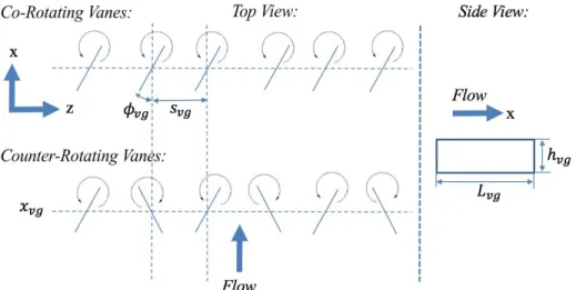
The planform of a rectangular vane was characterized by its height and length. The height is normalized by the thickness of the boundary layer (hvg/) and the length is normalized by the vane height (Lvg/hvg). Figures 6 shows the

planform of a vane. Figure 7 also shows the planform of a vane as placed in the STEX inlet. Traditional vane VGs have heights comparable to the boundary-layer thickness.15_{They entrain higher-momentum flow from outside the} boundary layer and create vortices that persist well downstream. Micro-VGs have heights comparable to half of the boundary-layer height.16_{Because of their smaller size and their presence in the lower-speed flow, micro-VGs have} less drag than traditional VGs. Placement of micro-VGs in supersonic flow have the benefit in that they avoid creation of shocks off of the VGs, which would create wave drag.

The vane axial placement is indicated by the x-coordinate xvg measured to the mid-point along the vane. The

angle-of-incidence of the vane vg relates the incidence with respect to the x-axis of the inlet. The right-hand-rule establishes

the positive orientation of the angle-of-incidence with respect to the normal to the inlet surface. The circumferential spacing is normalized by the vane height (svg/hvg).

An array of vanes is a grouping of a number of devices (Nvg) at an axial location (xvg) that span a specified

circumference of the interior surface of the inlet. The number of devices (Nvg) was determined based on the

circumference of the interior surface at the axial location and the spacing of the devices (svg). Figure 6 shows top

views of vane arrays. Figure 7 shows examples of vane arrays downstream of the shoulder of the STEX inlet. Figures 6 and 7(a) show counter-rotating vane arrays in which vanes alternate their angles-of-incidence between positive and negative values. Each pair of vanes create a pair of vortices that converge into each other. In the space between the pressure sides of the vanes, the flow rises from the surface and rolls about the edge of the vanes toward the suction sides. Counter-rotating vane arrays create symmetric vortex pairs that can be used to mix higher-momentum flow with lower-higher-momentum flow to energize the lower-higher-momentum flow in a uniform manner. This work will consider counter-rotating vane arrays.

Figure 7(b) show co-rotating vane arrays in which the vanes have negative angles-of-incidence. As the flow about each vane is directed from the pressure side of the vane to the suction side, the vane will create vortices with a counter-clockwise rotation based on the right-hand-rule with the inlet x-axis as the direction of the vortex. Figures 6 and 7(c) show a co-rotating array in which the vanes have positive angles-of-incidence. The vanes will create vortices that have a clockwise rotation. The pressure side of each vane of a co-rotating array is in-line with the adjacent vane so that the strength of vortices is not as strong as for the counter-rotating array. Although the co-rotating vane array could result in a more rapid decay of vortices than a counter-rotating array, it may be possible to establish the geometric factors such that the decay of vortices occurs at the engine face. The low-momentum region of the baseline inlet flowfield showed a non-uniform distribution about the circumference of the subsonic diffuser. Much of the low-momentum flow formed about the top of the subsonic diffuser downstream of the terminal-shock/boundary-layer interaction. A co-rotating vane array was considered for this work as a way of sweeping the low-momentum flow from the top down the sides of the subsonic diffuser.

(11)

11

American Institute of Aeronautics and Astronautics V. Results

Methods of the design of experiments (DOE) and statistical analysis were applied to perform fractional factorial screening studies to explore the significance of the factors for the vane arrays and reduce the number of factors to perform response surface methodology (RSM) studies to search for an optimum vane array for the STEX inlet. A. Quarter-Fractional Factorial Screening Study of Vane Arrays on the Subsonic Diffuser

A screening study explored the significance of the factors for vane arrays on the subsonic diffuser for improving the inlet performance measures. The five geometric factors for the vane arrays were vane height (hvg/), length

(Lvg/hvg), angle-of-incidence (vg), axial placement (xvg), and circumferential spacing (svg/hvg). The study included

vane arrays with orientations of co-rotating vanes with negative angle-of-incidence, co-rotating vanes with positive angle-of-incidence, and counter-rotating vanes arranged in pairs with alternating angles-of-incidence. A quarter-fractional factorial DOE design was used that involved the five geometric factors with two levels of each factor. Table 2 lists the low and high levels for each of the factors. This resulted in eight vane arrays or runs for a fractional design. This factorial design was repeated for each of the vane array orientations. Tables 3, 4, and 5 list the values of the factors for each run with respect to each vane array orientation.

A vane array was distributed about the upper 70% of the inner circumference of the subsonic diffuser at the axial location xvg in a similar manner as shown in Fig. 7. The boundary-layer thickness () at the axial location was

determined from the baseline inlet flowfield and varied along the circumference with the thickest boundary layer at the symmetry boundary at the top of the inlet. The height (hvg), length (Lvg), and spacing (svg) of the vanes was

determined using the local boundary layer thickness. Thus, these factors varied along the circumference.

Factors xvg_supersonic (ft) xvg_subsonic (ft) hvg/δ Lvg/hvg svg/ hvg vg (deg)

Low 0.05 0.4 0.5 2 3 8

High 0.10 0.8 1.0 3 5 16

The CFD simulations with the vane arrays used the refined grid 2 and the BAY model within the Wind-US flow solver. A grid interpolation method was used to determine the appropriate range of streamwise, transverse, and circumferential grid points containing each of the vanes as required as inputs to the BAY model. The grid interpolation method involved reading the information of the grid coordinates, establishing the values of the factors for a vane,

Figure 7. Vane arrays in the STEX inlet for (a) counter-rotating array, (b) co-rotating vane array with negative angles-of-incidence, and (c) co-rotating vane array with positive angles-of-incidence.

(12)

12

computing the polar coordinates of the vane, and converting the polar coordinates to the Cartesian coordinates. The vane planform area was calculated as input for the BAY model. The BAY model also required the angle-of-incidence. The quarter-fractional factorial DOE design of Tables 3, 4, and 5 have one value for the inlet performance measures for each of the eight vane arrays represented by a table. The values of the inlet performance measures for the row indicated as “Base” are those for the critical operating point of the baseline inlet flowfield for the refined grid 2 as identified in Fig. 4 and listed in Table 1. A goal of the DOE design and statistical analysis was to determine a better, if not optimum, vane array for the STEX inlet compared to the “Base”. The values of the inlet performance measures for each run as listed in Tables 3, 4, and 5 was obtained from the CFD simulation performed using the same outflow nozzle throat area as for the CFD simulation for the “Base”. Ideally, each run should be performed at the same engine-face corrected flow rate, which should be the same as that for the critical operating point of the baseline inlet flowfield. It was assumed that be using the same outflow nozzle throat area, that the corrected flow rates were “close enough”, if not the same. However, the corrected flow rate depends on the total pressure recovery and the total pressure recovery, as well as, the inlet flow ratio, varied for the runs. A check on whether a vane array is better than the baseline requires that the characteristic curve and distortion plots be generated for the inlet with the vane array and compared to the baseline. However, the generation of a characteristic curve requires several CFD simulations. Using equal outflow nozzle throat areas avoided performing multiple CFD simulations for each inlet with a vane array; however, it introduces some uncertainty as to the location of the solution on the characteristic curve. It was felt that this uncertainty was acceptable and that the search for an optimum vane array would still be valid. The discussion below will illustrate the approach.

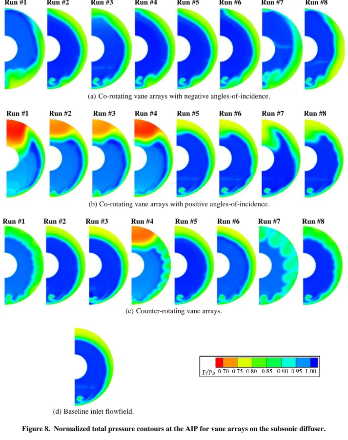
A qualitative examination of the effects of the vane arrays on the subsonic diffuser is presented in Fig. 8 which shows the contours of normalized total pressure at the AIP for each run. The runs with co-rotating vane arrays with negative angles-of-incidence shown in Fig. 8(a) indicate that they were effective in sweeping the low-momentum flow from the top of the AIP to the sides to re-distribute the low-momentum flow in comparison to the baseline flowfield. The runs with co-rotating vane arrays with positive angles-of-incidence shown in Fig. 8(b) seemed to sweep the low-momentum flow from the sides of the subsonic diffuser toward the top of the AIP. This was opposite of the desired effect of reducing the low-momentum flow at the top of the AIP. The runs with the counter-rotating vane arrays shown in Fig. 8(c) created vortex pairs that mixed the flow for some run (e.g. runs 1 and 8) or generated distinct vortex pairs that propagated downstream (e.g. runs 4 and 7). Figure 8(d) shows the contours for the baseline flowfield.

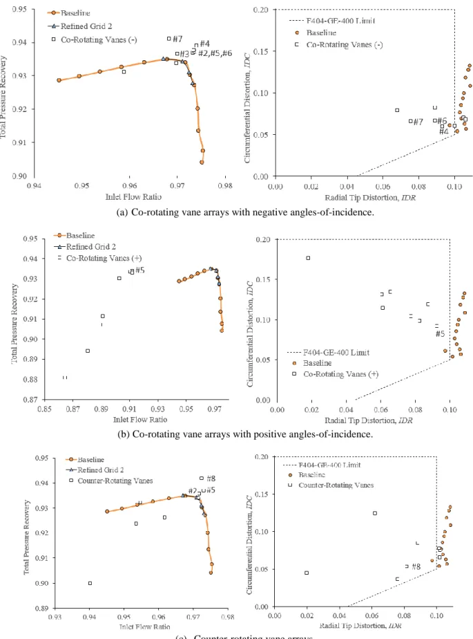
Figure 9 shows the characteristic curves and the distortion plots. The inlet performance measures for each run are also plotted. One can imagine that each data point for a run is one point on the characteristic curve for the inlet with the respective vane array. A “better” vane array would have a characteristic curve that is coincident or above and to the right of the characteristic curve of the baseline. This would mean that the vane array would provide the inlet with equal or higher total pressure recovery and inlet flow ratios. Thus, it was reasonable to make the decision that data points that fell below and to the left of the baseline characteristic curve do not represent acceptable vane arrays. This approach avoided having to perform multiple CFD simulations for each vane array, as proposed above. Thus, it is reasonable to all of the runs of Table 4 and runs 1, 4, and 6 of Table 5 from being acceptable vane arrays. The total pressure contours of Fig. 8 for these runs further lends support to this conclusion in that the total pressure distortion remains unchanged or worsens for these runs compared to the baseline. For some of these runs, the IDC and IDR

distortion descriptors are significantly reduced; however, the reduction in inlet flow ratio or recovery precludes these vane arrays despite the reduced distortion. The distortion plots show that almost all of the runs were able to reduce the IDR descriptors to within the limit line. All of the IDC descriptors remained below the limit line.

Of the runs that were not excluded, some runs showed promising vane arrays for improving recovery and reducing distortion. Runs 1, 7, and 8 of the co-rotating vanes with negative angles-of-incidence and runs 7 and 8 of the counter-rotating are included in this category. However, selection of a “best” vane array will be left to the response surface methodology (RSM) study of a later sub-section.

A statistical analysis was performed for each of the DOE factorial designs for vane arrays on the subsonic diffuser. The Design Expert software was used to perform the statistical analyses.17_{The purpose of the statistical analysis of} the quarter-fractional factorial was to determine which, if any, of the factors had a significant effect on the inlet performance measures (i.e. responses). The null hypothesis of the statistical analysis was that the factors had no effect on the responses. The analysis involved constructing a linear model of the response with respect to the factors. A quarter-fractional factorial with eight runs involved five degrees-of-freedom. An uncertainty level of 5% was chosen for the statistical analysis. The model and each factor was considered statistically significant if the uncertainty was less than 5%. In other words, there had to be less than 5% uncertainty that the variation of the responses due to a factor was due to noise in the responses. An analysis-of-variance was performed and the variances of the model and each factor were represented in the F-statistic, for which a probability for significance could be calculated and compared to the 5% uncertainty level.

(13)

13

For the fractional-factorial of co-rotating vane arrays with negative angles-of-incidence, a linear model for the total pressure recovery including just the factors (i.e. main effects) was first analyzed and found not to form a significant model. This meant that the best model for total pressure recovery was just the average of all eight values of recovery for the fractional factorial. Eliminating the factors with the lowest F-statistic improved the model, but a significant model was not obtained. A statistically significant linear model for IDR was obtained when only the factors height and angle-of-incidence were included. This model indicated that the angle-of-incidence was the most significant factor. The value of IDR decreased with an increase in the angle-of-incidence and height.

For the fractional-factorial of counter-rotating vane arrays, a statistically significant linear model was obtained for

IDR with respect to the factors of height and spacing. The vane height was the most significant factor with the trend indicating the higher vanes resulted in lower values of IDR. A statistically significant model for the total pressure recovery was not obtained; however, the height and axial position were suggested to have the most effect.

Runs xvg (ft) hvg/δ Lvg/hvg svg/hvg vg (deg) W2/Wcap pt2/pt0 IDC IDR

Base - - - - - 0.9710 0.9343 0.0857 0.0976 #1 0.4 1.0 2 3 -16 0.9588 0.9312 0.0794 0.0681 #2 0.8 0.5 2 3 -8 0.9732 0.9369 0.0705 0.1050 #3 0.8 1.0 3 3 -8 0.9700 0.9365 0.0602 0.0934 #4 0.4 1.0 2 5 -8 0.9740 0.9390 0.0605 0.1001 #5 0.4 0.5 3 5 -8 0.9736 0.9372 0.0682 0.1062 #6 0.4 0.5 3 3 -16 0.9734 0.9376 0.0667 0.0893 #7 0.8 1.0 3 5 -16 0.9683 0.9411 0.0659 0.0754 #8 0.8 0.5 2 5 -16 0.9698 0.9337 0.0827 0.0893

Base - - - - - 0.9710 0.9343 0.0857 0.0976 #1 0.4 1.0 2 3 ±16 0.9535 0.9237 0.0363 0.0759 #2 0.8 0.5 2 3 ±8 0.9718 0.9357 0.0746 0.1023 #3 0.8 1.0 3 3 ±8 0.9715 0.9341 0.0849 0.0885 #4 0.4 1.0 2 5 ±8 0.9402 0.8999 0.1244 0.0620 #5 0.4 0.5 3 5 ±8 0.9731 0.9369 0.0778 0.1017 #6 0.4 0.5 3 3 ±16 0.9618 0.9262 0.0657 0.1018 #7 0.8 1.0 3 5 ±16 0.9547 0.9321 0.0446 0.0198 #8 0.8 0.5 2 5 ±16 0.9725 0.9419 0.0535 0.0817

Base - - - - - 0.9710 0.9343 0.0857 0.0976 #1 0.4 1.0 2 3 16 0.8645 0.8807 0.1766 0.0180 #2 0.8 0.5 2 3 8 0.8896 0.9072 0.1190 0.0875 #3 0.8 1.0 3 3 8 0.8910 0.9113 0.1315 0.0606 #4 0.4 1.0 2 5 8 0.8806 0.8942 0.1348 0.0655 #5 0.4 0.5 3 5 8 0.9120 0.9339 0.0921 0.0925 #6 0.4 0.5 3 3 16 0.9107 0.9334 0.0986 0.0826 #7 0.8 1.0 3 5 16 0.9027 0.9301 0.1145 0.0612 #8 0.8 0.5 2 5 16 0.9120 0.9331 0.1039 0.0774

Table 3. Fractional factorial of co-rotating vane arrays with negative angles-of-incidence on the subsonic diffuser.

Table 4. Fractional factorial of co-rotating vane arrays with positive angles-of-incidence on the subsonic diffuser.

(14)

14

Run #1 Run #2 Run #3 Run #4 Run #5 Run #6 Run #7 Run #8

(a) Co-rotating vane arrays with negative angles-of-incidence.

Run #1 Run #2 Run #3 Run #4 Run #5 Run #6 Run #7 Run #8

(b) Co-rotating vane arrays with positive angles-of-incidence.

Run #1 Run #2 Run #3 Run #4 Run #5 Run #6 Run #7 Run #8

(c) Counter-rotating vane arrays.

(d) Baseline inlet flowfield.

(15)

15

American Institute of Aeronautics and Astronautics (a) Co-rotating vane arrays with negative angles-of-incidence.

(16)

16

B. Quarter-Fractional Factorial Screening Study of Vane Arrays on the Supersonic Diffuser

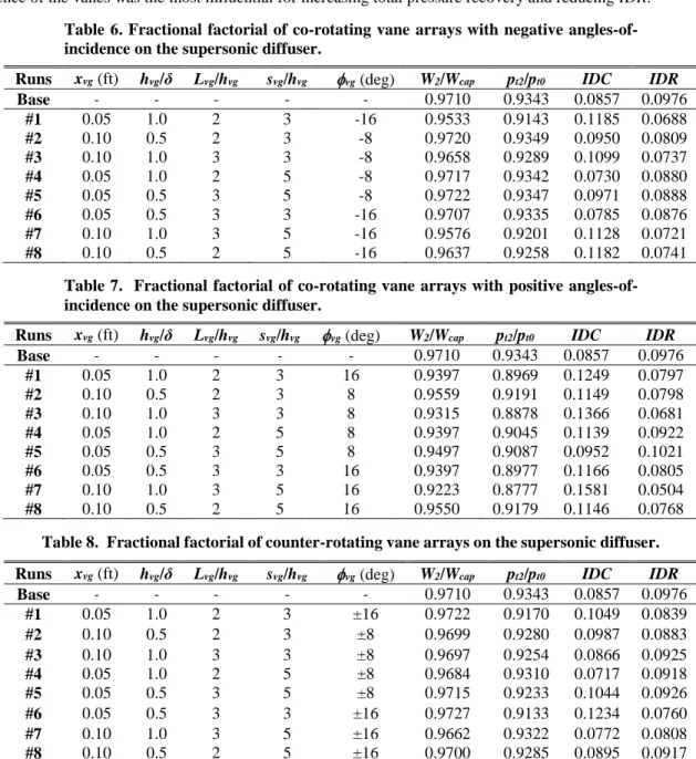
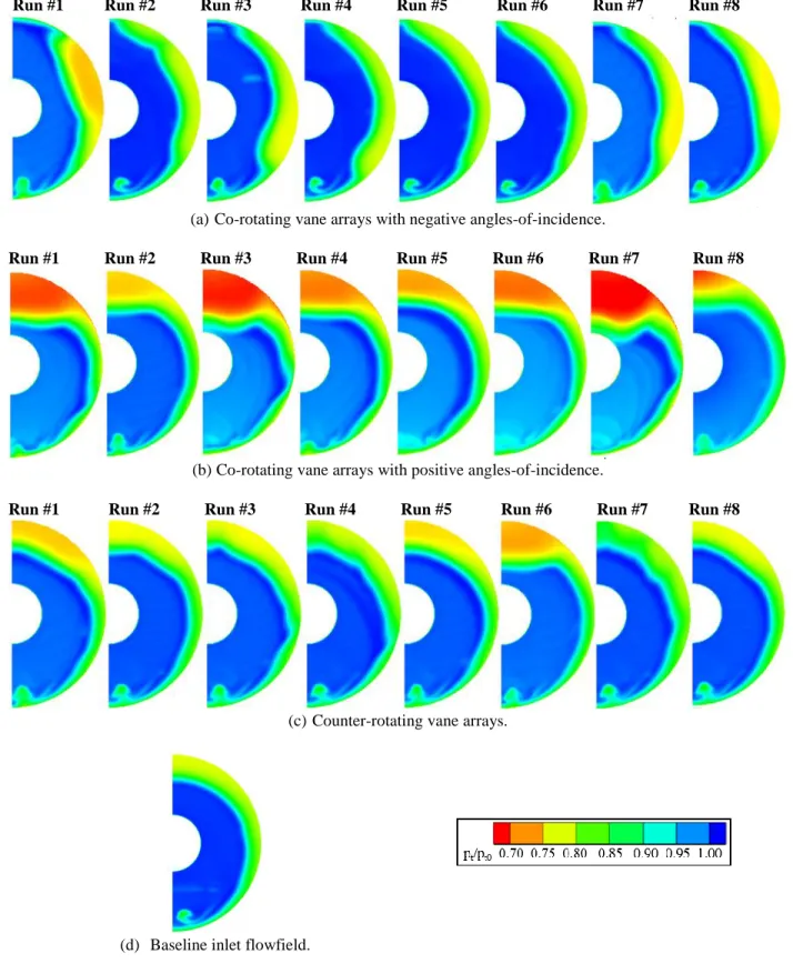
A quarter-fractional factorial screening study was performed for vane arrays on the supersonic diffuser. Table 2 lists the low and high levels for each of the five factors. Tables 6, 7, and 8 list the values of the factors for each run with respect to each vane array orientation and the inlet performance measures obtained from the CFD simulations. Figure 10 shows the contours of normalized total pressure at the AIP. The runs with co-rotating vanes with negative angles-of-incidence shown in Fig. 10(a) indicate they were effective in sweeping the low-momentum flow from the top of the AIP to the sides, which allowed high momentum flow to fill at the top of the AIP. The runs with the counter-rotating vanes shown in Fig. 10(b) and the runs with co-rotating vanes with positive angles-of-incidence shown in Fig. 10(c) did not have a positive effect.

Figure 11 shows the characteristic curves and the distortion plots. There was no improvement in total pressure recoveries; however, almost all of the runs yielded values of the radial distortion index IDR within the radial distortion limit of IDR = 0.10. The results suggest that only co-rotating vanes with negative angles-of-incidence are the acceptable approach for vanes on the supersonic diffuser.

The statistical analysis of the co-rotating vanes with negative angles-of-incidence was unable to produce a statistically significant model. However, the statistical analysis was able to suggest that the height and angle-of-incidence of the vanes was the most influential for increasing total pressure recovery and reducing IDR.

Base - - - - - 0.9710 0.9343 0.0857 0.0976 #1 0.05 1.0 2 3 -16 0.9533 0.9143 0.1185 0.0688 #2 0.10 0.5 2 3 -8 0.9720 0.9349 0.0950 0.0809 #3 0.10 1.0 3 3 -8 0.9658 0.9289 0.1099 0.0737 #4 0.05 1.0 2 5 -8 0.9717 0.9342 0.0730 0.0880 #5 0.05 0.5 3 5 -8 0.9722 0.9347 0.0971 0.0888 #6 0.05 0.5 3 3 -16 0.9707 0.9335 0.0785 0.0876 #7 0.10 1.0 3 5 -16 0.9576 0.9201 0.1128 0.0721 #8 0.10 0.5 2 5 -16 0.9637 0.9258 0.1182 0.0741

Base - - - - - 0.9710 0.9343 0.0857 0.0976 #1 0.05 1.0 2 3 16 0.9397 0.8969 0.1249 0.0797 #2 0.10 0.5 2 3 8 0.9559 0.9191 0.1149 0.0798 #3 0.10 1.0 3 3 8 0.9315 0.8878 0.1366 0.0681 #4 0.05 1.0 2 5 8 0.9397 0.9045 0.1139 0.0922 #5 0.05 0.5 3 5 8 0.9497 0.9087 0.0952 0.1021 #6 0.05 0.5 3 3 16 0.9397 0.8977 0.1166 0.0805 #7 0.10 1.0 3 5 16 0.9223 0.8777 0.1581 0.0504 #8 0.10 0.5 2 5 16 0.9550 0.9179 0.1146 0.0768

Base - - - - - 0.9710 0.9343 0.0857 0.0976 #1 0.05 1.0 2 3 ±16 0.9722 0.9170 0.1049 0.0839 #2 0.10 0.5 2 3 ±8 0.9699 0.9280 0.0987 0.0883 #3 0.10 1.0 3 3 ±8 0.9697 0.9254 0.0866 0.0925 #4 0.05 1.0 2 5 ±8 0.9684 0.9310 0.0717 0.0918 #5 0.05 0.5 3 5 ±8 0.9715 0.9233 0.1044 0.0926 #6 0.05 0.5 3 3 ±16 0.9727 0.9133 0.1234 0.0760 #7 0.10 1.0 3 5 ±16 0.9662 0.9322 0.0772 0.0808 #8 0.10 0.5 2 5 ±16 0.9700 0.9285 0.0895 0.0917

Table 6. Fractional factorial of co-rotating vane arrays with negative angles-of-incidence on the supersonic diffuser.

Table 7. Fractional factorial of co-rotating vane arrays with positive angles-of-incidence on the supersonic diffuser.

(17)

17

(a) Co-rotating vane arrays with negative angles-of-incidence.

(d) Baseline inlet flowfield.

(18)

18

American Institute of Aeronautics and Astronautics (a) Co-rotating vane arrays with negative angles-of-incidence.

(19)

19

American Institute of Aeronautics and Astronautics C. Response Surface Methodology Study for Vane Arrays on the Supersonic Diffuser

A response surface methodology (RSM) study was performed to search for an optimum vane array on the supersonic diffuser. The previous sub-section indicated that co-rotating vane arrays with negative angles-of-incidence were the only acceptable approach because they were able to sweep and redistribute the lower-momentum flow from the top to the sides of the subsonic diffuser. The statistical analysis of the fractional factorial suggested that vane height (hvg) and angle-of-incidence (vg) were the two most influential factors for reducing the radial distortion

descriptor, IDR. The vane arrays on the supersonic diffusers were not able to increase total pressure recovery. The sonic line of the boundary layer on the supersonic diffuser was approximately hvg/δ = 0.3. Thus, vane heights

comparable to hvg/δ = 0.3 were considered for the RSM study to keep the vanes mostly out of the supersonic flow to

avoid shocks and wave drag. The RSM study considered vane heights of hvg/δ = 0.3 to 0.7. The angle-of-incidence

was chosen to vary from vg = -12 to -20 degrees. These angles are higher than the fractional factorial studies and

chosen to expand the range of the fractional factorial studies. The RSM study involved three levels of the height and angle-of-incidence. Table 9 lists the low, middle, and high values of these two factors. The circumferential spacing was set at svg/hvg = 5.0 to reduce the number of vanes, which would simplify the vane array. The vane length ratio

was set at Lvg/hvg = 3.0 to allow the vanes more length to sweep the boundary layer flow. The position of the array

was set at the forward location of xvg = 0.05 ft.

With two factors and three-levels, a central-composite, face-centered DOE design was chosen. For two factors, this was also equivalent to a full-factorial. Table 10 lists for each run the values of the factors and the resulting inlet performance measures obtained from the CFD simulations.

Factors hvg/δ vg (deg)

Low 0.3 -12

Middle 0.5 -16

High 0.7 -20

Runs hvg/δ vg (deg) W2/Wcap pt2/pt0 IDC IDR Base - - 0.9710 0.9343 0.0857 0.0976 #1 0.3 -12 0.9721 0.9348 0.0937 0.0954 #2 0.7 -12 0.9723 0.9344 0.0792 0.0898 #3 0.3 -16 0.9720 0.9345 0.0931 0.0922 #4 0.7 -16 0.9588 0.9201 0.1276 0.0670 #5 0.7 -20 0.9623 0.9248 0.1228 0.0793 #6 0.5 -20 0.9597 0.9211 0.1163 0.0732 #7 0.5 -12 0.9719 0.9342 0.0889 0.0865 #8 0.5 -16 0.9713 0.9336 0.0757 0.0882 #9 0.3 -20 0.9717 0.9341 0.0891 0.0916

Figure 12 shows the contours of normalized total pressure for each run. Interestingly, when looking at the total pressure recovery at the AIP, two groups of similar solutions emerge: Runs one through three and seven through nine produce a region of low momentum flow stretching from the top of the AIP to roughly the 5 o’clock position. Runs four through six produce a strong region of low momentum flow, near the three o’clock position.

Figure 13 shows the points on characteristic curve and the distortion plot for each run. All of the runs improved the radial distortion relative to the baseline; however, improvements in total pressure recovery were minimal.

The statistical analysis of the results was performed using the Design Expert software and was not able to produce a statistically significant response surface model for the radial distortion (IDR). A 5% certainty was chosen and the statistical analysis indicated that there was a 6.7% chance that the F-statistic of 4.4 was due to noise. The model only included the main factors of the height and angle-of-incidence and no interactions or quadratic terms. The statistical analysis indicated that the height was the only significant factor. Contours plots of IDR with respect to the vane height and angle-of-incidence indicated that the lowest value of IDR could be obtained with the greatest height and angle-of-incidence. Statistically significant models could also not be produced for the total pressure recovery or the

Table 9. Low, middle and high levels of the factors.

Table 10. Response surface design for co-rotating vanes with negative angles-of-incidence on the supersonic diffuser.

(20)

20

circumferential distortion (IDC). Contour plots of these two responses indicate that the maximum total pressure recovery and minimum IDC could be obtained with the lowest values of vane height and angle-of-incidence.

The selection of the “best” vane array for the supersonic diffuser involved consideration of the results of the statistical analysis, as well as, engineering judgement based on the images of Fig. 12. Runs 4, 5, and 6 resulted in total pressure recoveries below the characteristic curve, and so, would likely not produce a characteristic curve better than the baseline even though the values of IDR were reduced the most. Runs 1, 3, and 9 with the vane height of hvg/δ

= 0.3 did not provide much reduction of IDR. A vane height of hvg/δ = 0.5 was considered to be better than a height

of hvg/δ = 0.7 to reduce possible wave drag from the vanes protruding into the supersonic flow. This left runs 7 or 8

with a vane height of hvg/δ = 0.5 as the choices for the “best” vane array. It was decided to select the middle level of

angle-of-incidence of vg = -16.0 degrees, which corresponded to run 8 as the “best” vane array. The contour for run

8 of Fig. 12 shows an acceptable redistribution of the low-momentum region.

Baseline Run #1 Run #2 Run #3 Run #4 Run #5 Run #6 Run #7 Run #8 Run #9

D. Response Surface Methodology Study for Vane Arrays on the Supersonic and Subsonic Diffusers

The studies of the previous sub-section on vane arrays on the supersonic diffuser indicated that a co-rotating vane array with negative angles-of-incidence had a positive effect on the radial distortion descriptor, IDR. A “best” vane

array with hvg/δ = 0.5 and vg = -16.0 degrees was established from the RSM study of the previous sub-section. It

seemed reasonable that a viable strategy for vortex generators in the STEX inlet would be to implement the above vane array on the supersonic diffuser to begin to improve the flow and then follow it with a vane array on the subsonic diffuser to further improve the flow. This is the approach of this sub-section.

A RSM study was performed to search for an optimum vane array on the subsonic diffuser in combination with the “best” vane array on the supersonic diffuser as discussed in the previous sub-section. The screening factorial

Figure 12. Normalized total pressure contours at the AIP for the response surface study of co-rotating vanes with negative angles-of-incidence on the supersonic diffuser.

Figure 13. The characteristic curve (left) and distortion plot (right) for the response surface study of co-rotating vanes with negative angles-of-incidence on the supersonic diffuser.

(21)

21

studies of vane arrays on the subsonic diffusers indicated that both co-rotating vane arrays with negative angles-of-incidence and counter-rotating vane arrays were acceptable for vane arrays on the subsonic diffuser. Since the vane array on the supersonic diffuser had a sweeping effect, it was decided to use a counter-rotating vane array in the subsonic diffuser to emphasize mixing over sweeping. The statistical analysis of the vane arrays on the subsonic diffuser suggested that the angle-of-incidence (vg), height (hvg/δ), and axial placement (xvg) were the most influential

factors. These three factors were chosen for the RSM study. Table 11 lists the low, middle and high levels of these three factors. The circumferential spacing was set at svg/hvg = 4.0 since it was the mid-point between the values of svg/hvg for the screening studies. The vane length was set at Lvg/hvg = 3.0. Table 12 lists the values of the factors for

each run and the inlet performance measures obtained from the CFD simulations.

Factors hvg/δ vg (deg) xvg (ft) Low 0.50 ±12 0.40 Middle 0.75 ±16 0.60 High 1.00 ±20 0.80

Runs hvg/δ vg (deg) xvg (ft) W2/Wcap pt2/pt0 IDC IDR

Base - - - 0.9710 0.9343 0.0857 0.0976 #1 0.50 ±12 0.4 0.9685 0.9345 0.0778 0.0687 #2 0.50 ±12 0.8 0.9612 0.9294 0.1094 0.0445 #3 0.50 ±16 0.6 0.9713 0.9374 0.0897 0.0755 #4 0.50 ±20 0.8 0.9564 0.9234 0.1287 0.0581 #5 0.50 ±20 0.4 0.9616 0.9270 0.1174 0.0574 #6 0.75 ±12 0.6 0.9684 0.9341 0.0983 0.0629 #7 0.75 ±16 0.4 0.9702 0.9361 0.0904 0.0683 #8 0.75 ±16 0.6 0.9700 0.9364 0.0847 0.0761 #9 0.75 ±16 0.8 0.9606 0.9227 0.1248 0.0679 #10 0.75 ±20 0.6 0.9693 0.9369 0.0807 0.0737 #11 1.00 ±12 0.4 0.9627 0.9249 0.1242 0.0732 #12 1.00 ±12 0.8 0.9602 0.9230 0.1048 0.0696 #13 1.00 ±16 0.6 0.9604 0.9230 0.1125 0.0624 #14 1.00 ±20 0.4 0.9622 0.9245 0.1240 0.0729 #15 1.00 ±20 0.8 0.9591 0.9217 0.1171 0.0660

The contours of the normalized total pressure at the AIP for each run are presented in Fig. 14. The contour of run 8 of Fig. 14 developed a reduced flow region half-way circumferentially in the inlet. Since the computations of the VG area depended on the boundary layer thickness, the vane area abruptly increased circumferentially in the reduced flow region, and then abruptly decreased outside of the reduced flow region. Circumferential trends will not be observed with VG height or VG area when placing subsonic VGs in conjunction with an upstream VG.

Figure 15 shows the total pressure recovery for each run on the characteristic curve plot and the total pressure distortion indices for each run on the distortion plot. Most of the runs were able to reduce the radial distortion IDR to values of about IDR = 0.6 to 0.7. Runs 2, 4, 5, 9, 12, 13, and 15 resulted in inlet flow rates and total pressure recoveries that were located below the baseline characteristic curve. The contours of total pressure recovery in Fig. 14 for these runs indicate pronounced regions of low-momentum flow that are likely responsible for the greater spillage and lower recoveries. Runs 11 and 14 did not show any improvement in any of the performance measures compared to the baseline flowfield. The remaining runs of 1, 3, 6, 7, 8, and 10 show similar improvements in all of the performance measures. These runs have vane heights of hvg/δ = 0.50 or 0.75 and axial placements of xvg = 0.4 or 0.6 ft. This

suggests that placing smaller vanes forward in the subsonic diffuser is beneficial. This allows ample distance for the vortices to decay prior to the engine face. A statistical analysis of response surface for IDR indicated that there was a 14% chance that the F-statistic of 2.1 was due to noise, which is above the 5% uncertainty limit. Thus an optimum

Table 11. Low, middle and high levels of the factors for the response surface design of a vane array for the subsonic diffuser.

Table 12. Response surface design of a counter-rotating vane array for the subsonic diffuser combined with a vane array on the supersonic diffuser.

(22)

22

vane array could not be established based on the RSM model. Based on all of the information of this study, the “best” configuration was selected to be run 1 with hvg/δ = 0.5, vg = 12 degrees, and xvg = 0.4 ft. With this selection the inlet

performance the IDC descriptor improved from IDC = 0.0857 for the baseline to IDC = 0.0778. The IDR descriptor improved from IDR = 0.0976 for the baseline to IDR = 0.0687.

Baseline Run #1 Run #2 Run #3 Run #4 Run #5 Run #6 Run #7

Run #8 Run #9 Run #10 Run #11 Run #12 Run #13 Run #14 Run #15

Figure 14. Normalized total pressure recovery contours at the AIP for the response surface study of co-rotating vanes on the supersonic diffuser combined with counter-co-rotating vanes on the subsonic diffuser.

Figure 15. The characteristic curve (left) and distortion plot (right) for the response surface study of co-rotating vanes on the supersonic diffuser combined with counter-co-rotating vanes on the subsonic diffuser.