Inter-American Development Bank Banco Interamericano de Desarrollo (BID)
Research Department Departamento de Investigación
Working Paper #598
Targeting the Structural Balance
by
Laura Dos Reis*
Paolo Manasse**
Ugo Panizza***
*Group of Twenty-Four
**World Bank
***United Nations Conference on Trade and Development
Cataloging-in-Publication data provided by the Inter-American Development Bank
Felipe Herrera Library
Dos Reis, Laura.
Targeting the structural balance / by Laura Dos Reis, Paolo Manasse, Ugo Panizza. p. cm.
(Research Department Working paper series ; 598) Includes bibliographical references.
1. Budget. 2. Fiscal policy. I. Manasse, Paolo. II. Panizza, Ugo. III. Inter-American Development Bank. Research Dept. IV. Series.
HJ2005 .D78 2007 350.722 D78----dc-22
©2007
Inter-American Development Bank 1300 New York Avenue, N.W. Washington, DC 20577
The views and interpretations in this document are those of the authors and should not be attributed to the Inter-American Development Bank, or to any individual acting on its behalf. This paper may be freely reproduced provided credit is given to the Research Department, Inter-American Development Bank.
The Research Department (RES) produces a quarterly newsletter, IDEA (Ideas for Development in the Americas), as well as working papers and books on diverse economic issues. To obtain a
complete list of RES publications, and read or download them please visit our web site at:
Abstract*
This paper discusses whether a country should conduct fiscal policy by targeting a structural (or cyclically adjusted) fiscal balance. The paper is divided into three sections. The first section discusses the concept of cyclically adjusted balance (CAB) and points out practical and conceptual problems related to the interpretation and the measurement of a CAB. The second section discusses the theoretical rationale for having a fiscal rule in general and a rule defined in terms of a cyclically adjusted balance in particular. The third section discusses conceptual and practical problems with adopting fiscal rules and rules that target the structural balance.
* Paper prepared for the XXIV Meeting of the Latin American Network of Central Banks and Finance Ministries, October 19th and 20th, Inter-American Development Bank, Washington DC.
1. Introduction
Political motivations and electoral considerations can distort fiscal policy. An often proposed mechanism for ensuring that debt policies are not biased by political influences is to rely on
fiscal rules that impose limits on unwarranted use of fiscal expansions. Fiscal targets including
balanced-budget laws and laws capping the size of the permissible deficit are sometimes included in fiscal responsibility laws that have been adopted in many Latin American countries over the past decade. These fiscal policy rules differ in the measure of fiscal performance that they involve (e.g., a strict ceiling or simply a target) and in provisions in case targets are missed. The range of performance indicators include the budget deficit, debt and public spending at various levels of the government. Some of the rules allow for margins around the target or time averaging to provide the opportunity to make up for shortfalls, and many allow for departures in case of international crisis or natural disasters.
Some authors point out that there are costs associated with such a policy framework. Rules are rigid; such is their nature. Under rare circumstances, such as an unusually severe recession, a financial crisis or a natural disaster, it may be desirable for stabilization purposes to cut taxes or increase public debt by more than in the typical downturn. Some rules do include “escape clauses” to provide for such contingencies. But this may raise problems of its own. Politicians who are inclined to use public spending to advance their re-election prospects will be tempted to cite an unanticipated contingency justifying a discretionary increase in spending whenever an election approaches. This problem can be ameliorated by assigning responsibility for declaring the existence of a relevant contingency to an independent, apolitical body but, in practice, it is difficult to delegate such functions to an extra-political body.
This paper discusses whether a country should conduct fiscal policy by targeting a structural (or cyclically adjusted) fiscal balance. The paper is divided into three sections. The first section discusses the concept of cyclically adjusted balance (CAB) and points out practical and conceptual problems related to the interpretation and the measurement of a CAB. The second section discusses the theoretical rationale for having a fiscal rule in general and a rule defined in terms of a cyclically adjusted balance in particular. The third section discusses conceptual and practical problems with adopting fiscal rules and rules that target the structural balance.
2. The Cyclically Adjusted Balance
One of the difficult aspects of assessing a country’s fiscal stance relates to the need to isolate changes in policy from the impact of temporary changes in economic circumstances (such as economic activity, inflation, interest rates or exchange rates). For instance, a sharp decline in the pace of activity may lead to a significant worsening of the fiscal situation without entailing any discretionary measures. If such a worsening is deemed to be temporary—assuming that the downturn is cyclical and likely to be reversed relatively quickly—and financing is available, there may not be any need for corrective measures.
The role of economic activity in influencing the budgetary position is acknowledged in the fiscal frameworks adopted in many emerging and industrial countries which conduct a routine and systematic assessment of the impact of changes in economic activity on the budget. The role of activity in influencing the government’s budgetary position is also acknowledged at the international level. The IMF, the OECD and the European Commission regularly publish figures for the cyclically adjusted balances of respective member countries.
“Structural” or “Cyclically-adjusted” balances (CAB) are typically calculated so as to remove the impact of the business cycle on the fiscal position and to provide a structural indication of the balance that abstracts from the temporary effects in the pace of activity. Thus the CAB asks the question “what part in the changes in the fiscal stance is due to changes in the environment and what part to changes in policy?”
Blanchard (1990) points out that there are five possible uses of the concept of cyclically adjusted balance and that having one indicator with multiple uses may be a source of confusion. The five uses highlighted by Blanchard (1990) are: (i) as an index of discretionary fiscal policy; (ii) as an index of permanent fiscal stance; (iii) as an index of how fiscal policy affects the economy; (iv) as an index of fiscal sustainability; and (v) as a policy goal. This paper focuses on the latter use of CAB.
There are several examples of countries that implicitly or explicitly target a CAB. In Chile, for example, the government targets a “structural balance” which reflects revenue adjustment for the “output gap” as well as for the price of copper (Franken, Lefort and Parrado, 2004; Valenzuela, 2006). Similarly, Poland, a recent EU member, includes in its annual budget a measure of the cyclically adjusted balance. In the European Union’s Stability and Growth Pact (SGP) there are provisions requiring fiscal outcomes to be close to balance or surplus over the
medium term, which is understood to encompass a full business cycle. The golden rule in the U.K. Code for Fiscal Stability states that, over the economic cycle, the government will borrow only to invest and not to fund current spending.1
2.1 Problems of Interpretation
Before discussing the practical problems associated with the measurement of CAB, it is worth recapping a few issues with the five standard interpretations of CAB listed before.
CAB as a measure of discretionary fiscal policy. Very often, changes in the CAB are interpreted as discretionary rather than non-discretionary policy responses, as opposed to non discretionary ones. The latter entails an automatic response of budget components to the economic environment (e.g., tax receipts responding to income, social payments responding to unemployment, debt servicing responding to interest rates, etc). Yet this interpretation is not fully warranted. It can be argued that the decision, say, not to modify tax rates in the wake of large and observable swings in the tax base is as discretionary as the decision to modify them. Thus “active” (or exogenous) versus “passive” (endogenous) policy responses seems a more accurate description of what the cyclical correction allows us to estimate.
CAB as a measure of structural policy stance. Another possibly misleading interpretation of the CAB is that it represents a permanent (“structural”) as opposed to a “temporary” (cyclical) change in the policy stance. This interpretation stems from the assumption that cyclical changes in output consist of random transitory deviations from a non-stochastic trend. Clearly, in the presence of stochastic trend shocks and structural breaks the CAB cannot be used to disentangle structural from cyclical components.
CAB as an indicator of the impact of fiscal shocks on the economy. Blanchard (1990) warns against using the CAB as a measure of how fiscal policy affect economic conditions. The possibility of inferring the impact of fiscal policy from changes in the balance is an ill-founded exercise as, even in the simplest Keynesian multiplier model, balanced budget changes (i.e., changes in expenditures matched by changes in revenue) imply a unit output multiplier. No
1 A more indirect way of taking into account the effects of the cycle in fiscal rules is through the use of contingency funds, which release resources to finance a cyclically induced deficit or withdraw them from a cyclically generated surplus. Examples of countries in which such countercyclical funds exist are Argentina, Peru and Estonia. In the United States, most states have so-called “rainy-days funds.”
simple statistics like the CAB can make up for a fully specified general equilibrium model of fiscal policy.
CAB as an indicator of fiscal sustainability. This is also a problematic interpretation because any given (primary) surplus, adjusted or not, can have very different implications for the dynamics of debt and its solvency depending on the relationship between the real interest rate, the rate of growth of the economy, and the debt structure. This is particularly problematic in emerging market countries where liquidity problems can soon become solvency problems (Calvo, 2005). Thus, relying exclusively on the budget balance is no substitute for comprehensive debt sustainability analysis.
CAB as policy target. Those who propose targets in terms of CAB argue that constant CABs are “good” for short-run stabilization or for long-run stability (Blanchard, 1990). Sections 2 and 3 of this paper will deal with this issue in greater detail. For the moment it is worth noting that while there is no theoretical argument for this conclusions, the policy implications of this interpretation seem to be akin to the popular statement that “automatic multipliers should be allowed to operate freely.” However, there is little reason to think that public savings should be at a given level on average, or to think that automatic stabilizers provide the optimal amount of stabilization. In fact, automatic multipliers operate very differently from country to country, depending on the structure of the tax and expenditure systems and on the size of spending and revenues over GDP (Fatàs and Mihov, 2001). Furthermore, automatic stabilizers cushion the economy against demand shocks, but may be counterproductive in so far they also dampen the economy’s response to supply shocks (Blanchard, 2000).
2.2 Problems of Computation of the CAB
The practical implementation of CAB is conceptually simple and usually consists of two steps. The first step decomposes output into trend and cycle components. The second step estimates the impact of the cycle on the budget (see Appendix 1 for a description of this two-step methodology).
A first problem with this simple two-step methodology is that it does not consider several factors that may affect the fiscal balance. In the two-step methodology illustrated in Appendix 1, the only variable employed for the adjustment is GDP. Normal conditions are identified with those prevailing when output is at its trend or potential level. The cyclical component of the
fiscal balance is obtained by multiplying the output elasticity of the budget by the deviations of output from trend/potential (output gap). The adjusted balance (CAB) is obtained residually. Such a procedure disregards the fact that there are several other variables that also affect the budget.
Four variables that are particularly important in emerging market countries are inflation, interest rate, commodity prices, and the real exchange rate. Inflation has an uncertain effect on the budget. On the one hand, the “fiscal drag” effect raises tax revenues because of incomplete inflation adjustment of tax brackets. On the other hand, the “Tanzi effect” reduces the real value of tax revenues because of collection lags. Interest rates are extremely volatile in emerging markets, and sudden jumps in country risk can lead to changes in the budget that are completely out of policymakers’ control (at least in the short-run). A standard solution to this problem is to focus on the primary balance.
Several emerging market countries are commodity exporters, and fluctuations in international commodity prices can have a strong impact on their budgets. In order to address this issue some countries incorporated adjustments for commodity prices into their fiscal policy framework. In Chile, for example, the central government targets a structural balance which reflects adjustments not only for the revenue effects of the output gap but also for those stemming from copper price deviations with respect to a reference price. (See Appendix 2.)
Fluctuations of the real exchange rate also affect the budget in a number of ways. The recent literature on “Original Sin” and Liability Dollarization, which has focused on the valuation effect of dollar-denominated debt, has shown that a large depreciation of the real exchange rate can push countries towards insolvency.
Finally, changes in CAB often occur due to the unfolding of budgetary implications of previous legislation. As examples, consider the budgetary implications of policy changes that are implemented through a gradual but predetermined schedule (e.g., progressive reductions in tax rates) or the gradual phasing in of a pension system, whereby expenditure grows “automatically” for a few years as new cohorts of retirees mature with higher claims then their predecessors.
The second problem is that, even if we forget all the complications listed above, the implementation of the conceptually simple two-steps methodology described in Appendix 1 is far from being trivial. We now discuss problems with each of the two steps: decomposition into trend and cycle and estimation of elasticities.
2.2.1 Decomposition between Trend and Cycle
Potential output is generally equated with trend output. Given a particular level of potential
output, actual output above the potential, that is, a positive output gap, means that the budgetary situation may be indeed worse than it appears, since revenues are high and expenditure low only for purely cyclical reasons. Similarly, a negative gap would imply that the budgetary situation may be better than it appears since the weak budgetary position is in part due to slower activity.
Trend-cycle decompositions are routinely undertaken in macro analysis. The basic idea is to decompose the output time series into the sum of potential output and a transitory deviation from it which is classified as cycle:
Observed Output= Trend Output + Cycle
This approach has a number of problems. First, as the constituent parts—trend and cycle—are not readily observed, any decomposition must necessarily be built on a conceptual artefact. Thus, any detrending method must start out by somehow arbitrarily defining what shall be counted as trend and as cycle, before these elements can be estimated from the data. As a
result, two major problems arise:
a) The various detrending methods proposed in the literature have dramatically distinct implications for the cyclical properties of the data (see Canova, 1999) b) Regardless of the method used, the decomposition is generally sensitive to
timing, in the sense that the decomposition can substantially change following (i) the extension of the sample period and (ii) data revisions (see, e.g., Figure 1 below, for an illustration of these effects).
The most common method used to extract the trend from a time series is the Hodrick-Prescott (HP) filter (Hodrick and Hodrick-Prescott, 1997) which is either applied directly to GDP series or to factors of production which are then combined into a production function (usually Cobb-Douglas) used to decompose output.2
2 The HP filter extracts the trend by finding a compromise between smoothness and fit of the estimated trend to the actual series (researchers can control this trade-off by choosing a smoothing parameter). The HP filter is one of the two methods used by the European Commission (EC) to generate cyclically-adjusted quantities, and it is also an integral part of the other method utilized: the production-function approach. In the production-function approach, trend-cycle decompositions are performed on labor and total-factor productivity series (no distinction between actual and potential capital is done). The Cobb-Douglas approach suffers from the standard criticism that it cannot accommodate change in the factor shares in output.
There is considerable evidence suggesting that, regardless of the methodology used, the estimates of the output gaps are generally subject to considerable margins of error, especially at the end of the sample period. Indeed, as noted earlier, revisions of the gap estimates are often of the same order of magnitude and may even exceed that of the gap itself (see below). There are two main sources of error in the concurrent estimation of the output gap:
First, there is the issue of the preliminary nature of the output data available in real time. Data revisions, which are typically non-negligible, will naturally result in output-gap revisions. This problem, however, will beset any methodology for correcting the balance for changes in activity. Second, and more relevant, most methods for estimating trend or potential output at any given time require future observations for a number of periods beyondthat time. This is because
most techniques employ symmetric (i.e., backward- and forward-looking) filters. In practice, since future observations are not yet available at the time of the calculation, truncated filters are used for the most recent observation. As observations become available, the past trend, and thus the output gap, gets revised, often substantially.
The above problems beset both industrial and emerging market countries.3 In the latter
case, however, the concept of a steady slowly-evolving trend around which the economy fluctuates is itself often difficult to ascertain because of the presence of greater, more frequent, and more persistent shocks. Indeed, emerging economies are often characterized by marked structural breaks. For example, Aguiar and Gopinath (2004) show that, unlike developed economies where output fluctuates around a relatively stable trend, shocks to trend growth are the primary source of fluctuations in emerging markets, thus blurring the simple distinction between trend and cycle.
Figure 1 provides an example of the implications of data revisions for the calculation of Brazil’s output gap in 1990 estimated with the standard HP filter and using World Economic Outlook data available at each point in time (see IMF, 2004). The graph shows that the variability of output gap revisions for the same year can be especially large in the years following the first estimate. In 1990 the gap was estimated at -3.5 percent; within two years it was seen to be only -2 percent; and the estimate converged only slowly to -2.5 percent over
3 Various studies have documented the difficulties of estimating the output gap in real time. For instance, for the U.S., Orphanides and van Norden (2002) show that the output gap revisions are of the same order of magnitude as the gap itself. Komaki (2003) arrives at the same conclusion for Japan, and cautions against using real-time estimates as the basis for policy.
subsequent periods. It is worth noting that this change occurred because the revision in estimates of the level (and growth) of output not only modified the values of the actual level, but also caused a substantial revisions on the estimates of potential output. As a result, even the past levels of the gap were affected.
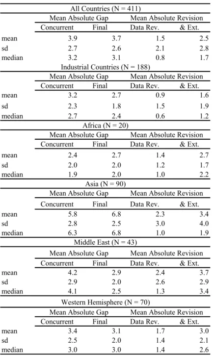
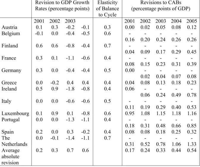
Such large changes in the estimates of the output gap will obviously lead to corresponding changes in the estimates of the cyclically adjusted fiscal balances. IMF (2006) estimates gaps for each year based on information available at the time by using the WEO two-year projections available at each date for calculating the trend. This estimate (the “concurrent” gap) is compared with the “final” estimate, which incorporates five more years of data. The results are summarized in Table 1. The mean absolute revision (1.5) amounts to 47 percent of the mean absolute gap (3.4). About 93 percent of the revision is due to data revisions, and only the remaining 7 percent is due to extending the data series. The revisions are relatively larger in Western Hemisphere countries, where they amount to 90 percent of the final absolute gap, and smaller in Asia: 35 percent of the final gap. The output gap revisions carry over to the revisions in the CAB. González-Mínguez, Hernández de Cos and del Río. (2005) and IMF (2006) illustrates the impact of GDP revisions on the CABs for EMU members by comparing estimates for different years from two EC releases only six months apart: the Spring 2003 vs. Autumn 2003 releases (Table 2). Minimal gap revisions (e.g., those for Spain) have a significant impact on the CABs for the current and subsequent years.
2.2.2 Budgetary Elasticities
The second step of the standard procedure for computing CABs requires the estimation of output elasticities for revenue and expenditures. These estimates are subject to uncertainty and can be prone to structural breaks, resulting in changes to the CAB, even if the output gap estimates are not revised.
Typically, the revenue and expenditure elasticities are obtained by regressing the rate of growth of the relevant items on the rate of growth of output. The elasticities calculated in this way are then applied to the output gap in order to derive CABs. In principle, this procedure, by disaggregating the structural balance into its components, allows an analysis of the composition effect of output changes on revenues and expenditures separately, and this provides useful information. This methodology may be worthwhile when the revenue and expenditure elasticities
change in opposite direction. Suppose that a reform makes the tax system less progressive and unemployment benefits more generous: revenue will fall less and expenditures will rise more in a recession, and the opposite will occur in a boom. If the correct estimates are employed, the reliability of the estimated balance will improve. However, should the tax and the expenditure elasticities change in similar direction, the aggregate estimate would become less reliable.
A similar issue arises for the effects of changes in output compositions on budget elasticities. Momigliano and Staderini (1999), for instance, compute trend values for macroeconomic variables which represent good proxies for tax bases whose impact on public finances is particularly large. They argue that the effects of changes in composition can be large, seriously undermining the reliability of aggregated procedures and support their argument with evidence from Italy. A similar point is made by Langenus (1999) for Belgium. The computation of CAB based on trend values for GDP components is currently applied by the European System of Central Banks. Whether these procedures generate budget elasticities which are more robust to breaks and structural changes is ultimately the empirical question that needs to be addressed.
3. The Case for a Structural Balance Target
Recent developments in the US, where the budget has plummeted from a surplus to a record peacetime deficit, and in Europe, where the Growth and Stability Pact has been loosened in order to accommodate systematic violations of the deficit-to-GDP limit by large countries in recession, have renewed interest in institutional restrictions on fiscal policy.
A large variety of fiscal rules exist. Some focus on numerical targets or rules and apply to different aggregates (borrowing, expenditures, primary balance), while others involve procedural and transparency requirements. Additional differences involve the extent of coverage (e.g., federal and/or state governments), the presence of escape clauses, and the presence of explicit sanctions. Many countries have also introduced medium-term budget frameworks and “fiscal responsibility laws” (see IMF, 2006). Some authors have even advocated the delegation of fiscal policy to independent Fiscal Councils (Wyplosz, 2005), for reasons akin to the delegation of monetary policy to independent Central Banks.
There are two opposite views about the desirability of such rules. These views reflect the standard trade-off between credibility gains and the loss of stabilization that such rules may entail. Opponents argue that fiscal rules limit the ability of the government to stabilize the
economy and thus foster procyclicality. This idea goes back to the criticism of the European Stability and Growth Pact (see Buiter et al., 1993). Poterba (1994), Alt and Lowry (1994), and Roubini and Sachs (1989) document how fiscal constraints inhibit the reaction of policy to unexpected shocks. Put simply, when the economy is hit by a bad shock, the deficit (or debt)-GDP ceiling becomes binding, requiring a procyclical fiscal adjustment (higher taxes and/or expenditure cuts in a recession).
Those in favor of rules argue that, rather than being benevolent, governments are subject to political distortions that make them run excessive deficits. Therefore rules that limit policy discretion can achieve a desirable intertemporal path of tax rates and a sustainable level of debt and reduce a potentially important source of macroeconomic volatility.
In a simple Barro-Gordon framework, Manasse (2005) rationalizes the idea that deficit-to-GDP limits, involving a linear (stochastic) penalty when breached, entail a trade-off between the benefits of reducing the average deficit bias, which is assumed to be politically motivated, and the costs of foregone stabilization (to which the expected penalty must be added when the stabilization requires a violation of the limit). As a result of the fiscal constraint, the optimal policy becomes state-contingent: in moderately bad times, the constraint is reached and the government optimally chooses to keep the deficit-to-GDP ratio as close as possible to the limit in order to avoid the penalty (fiscal policy is “acyclical”). However, during economic slumps, the cost of foregoing stabilization exceeds the expected penalty from breaking the rule, so that the government chooses to violate the rule and runs an expansionary (countercyclical) policy.
Clearly, the policy implications of fiscal rules depend very much on the details of their design. “Well-designed” rules may reduce the deficit bias and foster, rather than inhibit, an appropriate (countercyclical) policy. A rule that penalizes deficits and also rewards surpluses,
say by means of a stabilization fund, provides incentive for the government to raise surpluses in good times in order to accumulate “credits” to be spent in bad times (Manasse, 2005). The same result would be achieved by allowing governments to exchange deficit “permits” (see Casella, 1999).
In a similar vein, Tanner (2004) discusses a dynamic model where policymakers are subject to an electoral distortion and prefer current to future consumers (voters). In this context, well-designed fiscal rules may reduce the need for future increase in tax rates, thereby allowing
policymakers to better smooth tax distortions over time, reduce procyclicality, and improve welfare.
Summing up, the theory suggests that fiscal rules should be associated with a lower average deficit, but the effect on output volatility is ambiguous, and depends on the actual design of the rule, the nature of the political distortion, and the time horizon of policymakers.
Making the case for adopting a fiscal policy framework based on a structural balance target requires two logical steps. The first consists of establishing that a budget rule can be superior to discretion. The second consists of establishing that a rule in terms of a structural balance is superior to both discretion and a simple rule based on the actual balance.
3.1 Fiscal Rules and Procyclicality
Procyclical fiscal policies, that is policies that are expansionary in booms and contractionary in recessions, are generally regarded as potentially damaging for welfare: they raise macroeconomic volatility, depress investment in real and human capital, hamper growth, and harm the poor (Inter-American Development Bank; 1995, Servén, 1998; World Bank, 2000; IMF, 2005a; IMF 2005b). Moreover, if expansionary fiscal policies in good times are not fully offset in bad times, they may also produce a large deficit bias and lead to unsustainable debt dynamics and eventual default.
The finding that fiscal policies tends to be procyclical is puzzling, since it does not square with the common wisdom that governments should borrow in “bad times” when revenues shrink and “social” spending rises, and repay debt in good times. More specifically, procyclical fiscal policy is at odds with both the neoclassical notion that tax policy should be used to smooth tax distortions and expenditures over the business cycle—provided shocks to the tax base or spending are temporary—and the Keynesian notion that taxes and expenditures should try to dampen, rather than exacerbate, business cycle fluctuations.
Gavin and Perotti (1997) were the first authors to document that budget deficits in Latin America in 1970-95 largely failed to respond to economic growth, suggesting that discretionary policy was used in a procyclical fashion, so as to offset automatic stabilizers (for example, raising expenditures to offset revenue windfalls in good times). They suggested that the explanation might relate to the fact that capital flows are also strongly associated with the business cycle: they tend to be high in good times and low (or negative) in bad times. The idea
that developing countries may face borrowing constraints, in bad times but not in good times, is also supported by the evidence presented in Kaminsky, Reinhart and Végh (2004). In particular, they show that credit ratings for Latin American sovereign issuers tend to be good during periods of high growth and bad during recessions.
Other studies present evidence of procyclicality for developed countries as well, albeit to a lesser extent. For example, IMF (2005a) finds that a one-point increase in the output gap (defined as the percentage deviation of actual from potential output) in these countries is on average associated with an improvement of the overall deficit ratio by 0.3 percent in industrial countries. Given the evidence that automatic stabilizers are estimated to improve overall budget performance by 0.5 percentage points (van den Noord, 2000; Bouthevillain et al., 2001; IMF, 2005a), this result suggests that discretionary policy has been used procyclically in developed countries as well.
A related finding is that fiscal policy is asymmetric over the business cycle and that this is especially the case in developed economies. For instance, European Commission (2001) finds that in 1970–2000 European countries let the overall deficit widen in downturns, but failed to reduce it in upturns. Hercowitz and Strawczynski (2004) find a similar “cyclical ratcheting” effect for government spending in OECD countries, while Balassone and Francese (2003) and Buti and Sapir (1998) confirm these results for OECD and EU countries, respectively. Manasse (2006) finds that, both developed and developing countries, fiscal policy is “acyclical” (that is, the ratio of the primary balance to GDP does not respond to the output gap) in bad states of nature and becomes procyclical in good times.
While Gavin and Perotti (1997) argued that the difference in procyclicality between Latin American and OECD countries was due to the presence of borrowing constraints, successive work has focused on weak institutions, corruption, asymmetric information, “voracity effects,” and common pool problems.4
4 Lane and Tornell (1999) discuss a “voracity” effect that may take place in economies lacking strong legal and political institutions. In such circumstances, a windfall in revenue exacerbates the struggle for fiscal redistribution, as each interest groups tries to appropriate its share without fully internalizing the consequence of its own demand on general taxation. Lack of coordination, in this version of the familiar common pool problem, is ultimately responsible for a more-than-proportional increase in spending. Talvi and Végh (2005) present an optimizing behavior model that introduces a political distortion, which raises the cost of running surpluses in good times. They show that, a result, the government will choose to cut tax rates in good times to fend-off spending pressures in bad times. Although this distortion is not derived explicitly, it is supposed to capture political pressures and weak institutions. Alesina and Tabellini (2005) suggest an explanation for procyclical fiscal policy based on voters’ mistrust of corrupt politicians. Voters are not fully informed of government transfers and borrowings, but observe
An implication of this “institutional” approach is that countries in which budgetary power is diffused among a number of agents will experience higher degrees of fiscal procyclicality. However, empirical support for this hypothesis is not clear-cut. For instance, Lane (2003) finds that the measure of political constraints developed by Henisz (2002) has a weak impact on the degree of procyclicality. An institutional factor which can impact on the degree of procyclicality is the structure of local governments. Braun and Di Gresia (2003), for instance, argue that the federal government system contributes to fiscal procyclicality in Argentina. This is linked to the fact that taxes raised by local governments (provinces) are less revenue elastic than federal taxes. Provinces’ revenues are therefore very pro-cyclical. Furthermore, because of the ‘common pool’ problem, provinces also have incentives to overuse common resources, thus implementing very procyclical spending. This behavior is reinforced by a history of federal bailouts, which reduce incentives for fiscal prudence during booms.
Calderón, Duncan and Schmidt-Hebbel (2005) focus on 20 EM countries and also find that procyclicality depends on institutional quality (countries with higher levels of institutional quality are less procyclical). Akitoby et al. (2004) find that procyclicality tends to be lower in richer countries with less concentrated political power, lower ICRG ratings of financial risk (an indicator that proxies for institutional quality), and larger public sectors. Braun (2001) also finds that public sector size is an important determinant of procyclicality and that transfers act as
output accurately. Since they cannot prevent the government from borrowing in good times, they will demand lower taxes and more consumption in such times, as they (correctly) anticipate that, otherwise, windfall revenues will be dissipated through unproductive rents. Guerson (1993) proposes an interesting model that can combines elements of both the “institutions” and “rule/constraints” view. In an overlapping generation model where the government acts as a benevolent planner, he shows that a procyclical policy can be socially optimal when the government cannot commit not to default on its debt. Since the temptation to default is higher in bad times, the risk premium is also higher in such states. Thus, following a negative shock, the government does not fully accommodate it by borrowing, which would raise the risk premium considerably, and finds it optimal to partially reduce spending. This mitigates the rise in interest rates and the fall in future consumption. Riascos and Végh (2003) argue that the lack of a sufficiently rich menu of financial assets might be a major determinant of procyclicality in developing countries. Under this explanation, even assuming full access to capital markets, the inability to borrow contingent on the economic situation reduces the economy’s diversification of its idiosyncratic risk, leading to a positive correlation between government spending and the cycle. For similar reasons Borensztein and Mauro (2002) suggest the adoption of GDP-indexed bonds, which would pay lower interests during recessions, thus reducing the need for adjusting spending in bad times. A similar rationale is behind the proposal of issuing Government-Revenue Indexed Bonds with IFI credit lines contingent on recessions. Another possible explanation (see Galiani and Levy-Yeyati, 2003) is that procyclicality occurs because fiscal spending converges over time to a desired spending level determined by long-run fundamentals and that the speed of convergence increases with the distance between desired and actual spending. In this setting, procyclicality is generated by the fact that convergence is faster during booms than during recessions, suggesting that governments in economies with postponed public consumption are hard-pressed to spend whatever windfall they receive almost immediately.
automatic stabilizers and reduce procyclicality. Similar results are found by Manasse (2006) for a large sample of developed and emerging economies.
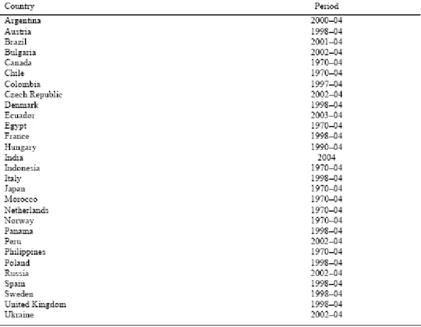
There are only few formal tests of the effects of fiscal rules on the procyclicality of fiscal policy. Manasse (2006) constructs a dummy for the presence of a “fiscal rule” in each country-year in a sample of 49 developed and emerging economies (Table 3 lists the episodes of fiscal rules in the sample).5 A “policy reaction function” of the fiscal authority is estimated by OLS
according to the following specification:
Sv,t = a0 + a1 Gapv, t-1 + a2 Debtv, t-1 + a3 Sv, t-1 +
+ a4 FRv,t + a5 FRv,t Gapv, t-1+ a6 Xv,t-1 + uv,t . (1)
where Sv,t is the primary surplus of the general government expressed as a ratio of GDP in country v at time t, Gap v,t is the output gap, Debt v,t is the ratio of the stock of public debt over GDP, FR v,t is the dummy indicating the presence of a Fiscal Rule in country v at time t, and X represents a vector of other controls, including country fixed effect.
The constant, a0, can be interpreted as a measure of the deficit (if negative) bias, namely the average balance that is left after controlling for the reaction of the surplus to the debt and the output gap. A positive coefficient a1 means that the surplus rises in good times, indicating a countercyclical stance. A negative estimate of a1 signals a procyclical policy. Finally, the average effect of the Fiscal Rule (FR) is captured by the coefficient a4. If this coefficient is positive, it means that the presence of a Fiscal Rule (FR=1) is associated with a higher surplus (a lower deficit bias). A positive coefficient a5 suggests that the FR enhances the countercyclical response of the surplus to the output gap, while a negative estimate suggests that a FR aggravates the procyclical nature of the policy.
The results are reported in Table 4. They suggest that fiscal policy is on average subject to a deficit bias of roughly 1.5 percent of GDP (a0=1.5);that fiscal policy is weakly procyclical (a1 is negative and significantly different from zero); that FRs tend to reduce the deficit bias (a4=0.66) by roughly two-thirds of a percentage point of GDP; and that fiscal rules make policy more counter rather than pro-cyclical (a5 is positive). These results have a simple interpretation:
5 Following Kopits and Symansky (1998), a fiscal rule is defined as a “... permanent constraint on fiscal policy, typically defined in terms of an indicator of overall fiscal performance...such as the government budget deficit, borrowing, debt, or major components thereof—often expressed as a numerical ceiling or target, in proportion of Gross Domestic Product.”. Fiscal responsibility laws are also considered. Alternative sources, such as the OECD-World Bank (2003) detailed survey on Budget Practices and Procedures, lack a time dimension.
if fiscal discretion is a source of macroeconomic instability, the constraints posed by fiscal rules actually inhibits a destabilizing policy, rather than preventing a stabilization policy.
Evidence from other studies seems to corroborate this interpretation. Fatàs and Mihov (2003) for a sample of ninety nine countries find that government spending is an important source of output volatility. In a different study on US States, the same authors present evidence that support the presumption that budgetary restrictions are associated with lower expenditure volatility, which they interpret as a measure of discretion, and that this effect dominates the inhibiting effect on the ability to stabilize output fluctuations (Fatàs and Mihov, 2006). Galì and Perotti (2003) find that since the Maastricht treaty and the SGP, discretionary fiscal policy in EMU countries has become more countercyclical over time, following what appears to be a trend that affects other industrialized countries as well.
A possible problem with rule-based fiscal regimes is that they may limit the possibility of conducting countercyclical policies and hence increase output volatility. Whether this is the case is, by and large, an empirical question. While Manasse (2006) finds that fiscal rules reduce procyclicality, his estimations bunch together several types of budget rules and hence cannot say anything about the effect of a specific fiscal rule like a structural balance rule.
Devising a test aimed at evaluating the effect of a structural balance rule is complicated by the fact that very few countries adopt such a rule (see Appendix 2 for a description of the Chilean rule). Dos Reis and Guerson (2006) try to overcome this limitation by simulating the effect of imposing a structural balance rule on a sample of five Latin American countries (Argentina, Brazil, Colombia, Mexico, and Uruguay). In their experiment, they compare the volatility of a vector of variables as estimated from two Monte Carlo simulations based on a VAR model to study how these economies would have behaved had they been able to implement a structural balance expenditure rule.6 In particular, they adopt the following procedure. They
start by simulating the volatility of the cyclical component of GDP obtained by estimating an unrestricted VAR and comparing it with the volatility of GDP obtained by estimating a VAR where government expenditure is set equal to a fixed percentage of long run government revenues.
6 The variables included in the VAR are capital flows as a share of GDP, the cyclical components of GDP, primary expenditure, government revenues, and the real exchange rate. This choice of variables comes from the empirical evidence that procyclical fiscal policy is driven by the procyclicality in capital flows (see Kaminsky, Reinhart and Végh, 2004).
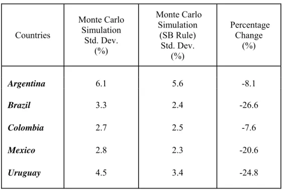
Table 5 summarizes the findings of Dos Reis and Guerson (2006) and shows that the structural rule described above should always reduce GDP volatility. The effect appears to be extremely large for Brazil, Mexico and Uruguay (where volatility decreases by more than 20 percent) and much smaller in Argentina and Colombia.
While this simple exercise provides some suggestive results on the potential impact of imposing a structural balance, it is worth mentioning that there are several problems with the VAR simulation described above. The main issues are: (i) the VAR exercise uses past data and hence can only estimate past trend revenues and completely disregards the forward-looking nature of any policy aimed at imposing a structural balance; (iii) the exercise assumes that the various elasticities are stable and can be estimated (allowing feedback). Hence, the results discussed above should be interpreted with caution.
4. The Case for Discretionary Fiscal Policy
The previous section argued that balanced budget rules in general, and structural balance rules in particular, can eliminate the deficit bias that characterizes the political system in several countries while allowing for the presence of a countercyclical fiscal policy. This section argues that there might be practical and conceptual problems with the implementation of a fiscal policy framework based on a structural balance.
In particular, we consider three issues: (i) A structural balance target may impose unnecessary constraint on virtuous politicians during good times; (ii) Fiscal rules can be the
source of creative accounting, and structural rules may make the problem worse; and (iii) Even if respected and effective, rules aimed at a structural balance target may not be successful at preventing debt explosions and procyclical fiscal policy.
4.1 Unnecessary Constraints on Virtuous Politicians
The finding discussed in the previous section that fiscal rules are associated with less procyclical fiscal policy does not imply that fiscal rules are necessarily a panacea, reducing the average deficit bias and improving the policy response to the business cycle. The reason is that fiscal rules may be endogenous. It is more likely that virtuous countries/governments put in place fiscal frameworks that are conducive to fiscal sustainability and to a correct policy response to the cycle, rather than being such frameworks that make countries/governments more virtuous. It is
easy to find loopholes in any rule in the absence of the political will to abide by it (the EU Stability and Growth Pact docet).
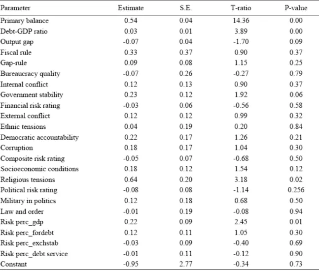
The evidence seems to confirm this intuition: fiscal frameworks may be themselves determined by “deeper” institutional variables, so that they do not significantly affect policy when the quality of institutions is controlled for. Table 6 introduces institutional variables into equation (1). These include indexes of the quality of government, the presence of internal and external and religious conflict, civil rights, law enforcement, corruption, perception of risk for growth, for solvency, exchange rate risk and so on (a higher value represent better institutions).
The striking feature of this table is that while the coefficients on the output gap and debt ratio remain virtually unaffected, the Fiscal Rule dummies in level and interaction become insignificant when these institutional variables are accounted for. Among the newly added variables, the index of Government Stability and the index of (lack of) Religious Tensions are significant and with the expected positive sign, indicating that better institutions are associated with higher average balances. This finding indicates that the presence of a fiscal rule is only a proximate cause of countercyclical policy. Countries with good institutions conduct countercyclical policies and decide to endow themselves with a set of fiscal rules.
Clearly, this just says that fiscal rules might be useless but does not say anything about possible harmful effects of a fiscal rule. Consider, however, the case of a country governed by fiscally conservative policymakers who are under constant pressure to expand public expenditure (one may think of a game in which a fiscal conservative Minster of Finance needs to resist pressures from the legislative assembly). If there are no changes in trend growth, a structural balance target may have beneficial effects and afford the fiscally conservative policymaker sufficient ammunition to keep expenditure under control. But a fiscal rule can be a double-edged sword. Assume now that the (possibly independent) commission that is in charge of estimating trend output deems that the country went through a structural break and that trend growth has increased (an upward revision of the long-run price of a commodity exported by the country would have a similar effect). In such a situation, the fiscally conservative policymakers will be forced to jump immediately to a new level of trend expenditure, and this may cause several problems. First, the sudden jump may overheat an economy which is already growing at a fast rate. Second, the country may not have the ability to properly manage a sudden increase in public expenditure. Finally, if the experts prove to be wrong and GDP growth reverts to its previous
(lower) level, the country will end up with a hard-to-reverse higher level of public expenditure. This problem is particularly important in emerging market countries, which are characterized by high output volatility, and where it is extremely difficult to separate the cycle from the trend (Aguiar and Gopinath, 2004).
Things would be different if policy were discretionary and set by a fiscally conservative policymaker. In this case, the policymaker will attempt to smooth any change in policy. If, indeed, the country is moving towards a new path of higher growth, the policymaker will slowly adjust expenditure towards a higher level (assuming that there are good reasons to increase expenditure), but if the increase in growth ends up being temporary, the policymaker will slowly revert expenditure towards its previous level.
Summing up, structural balance rules can be good when it is easy to separate the trend and cyclical component of output, but this is rarely the case in emerging market countries. Even in cases in which it is not easy to separate the trend and cyclical component of output, structural balance rules can play a useful role in constraining fiscally irresponsible policymakers. However, rules may make the situation worse in presence of fiscally responsible policymakers. The problem is that Manasse’s (2006) result seems to suggest that only fiscally responsible politicians decide to adopt budget rules.
4.2 Creative Accounting
Budget rules imposed in countries that do not have a transparent budget process may lead policymakers to engage in creative accounting practices (Milesi-Ferretti, 2004) which, by creating “skeletons in the closet,” will ultimately have negative effects on a country’s ability to conduct an optimal fiscal policy. It is not clear whether rules that target the structural balance will increase or decrease the incentive (with respect to a rule aimed at the current budget balance) to resort to creative accounting practices. On the one hand, the greater flexibility of the structural rule may give policymakers some leeway and reduce their incentive to trick the data. On the other hand, structural balance rules are more complex than rules based on the current balance and are therefore easier to manipulate.
Hence, fiscal rules may end up reducing the transparency of the policymaking process in general and of public accounts in particular. This is bad for every country but may hold a particularly high cost for cost for emerging market countries where there is evidence that the
transparency of public accounts is closely related to borrowing costs and the probability of sudden stop episodes.7
4.3 No Help in Reducing Procyclicality and Debt Explosions
The standard rationale for adopting a fiscal rule is to tackle the deficit bias that leads to continuous debt growth and the rationale for defining a rule in terms of structural budget is to address the deficit bias while guaranteeing a countercyclical fiscal policy stance.
4.3.1 Deficit and Debt
The idea that by controlling the deficit one can control debt growth may seem trivial. After all, the standard Economics 101 debt accumulation equation states that the change in the stock of debt is equal to the budget deficit:
t t
t DEBT DEFICIT
DEBT − −1 = (2)
and that the stock of debt is equal to the sum of past budget deficits:
∑
= − = t i i t t DEFICIT DEBT 0 . Whoever has worked with actual debt and deficit data knows that Equation (2) rarely holds and that debt accumulation can be better described as:
t t t
t DEBT DEFICIT SF
DEBT − −1 = + (3)
where SFt is what is usually called “stock-flow reconciliation.” Clearly, Equation (2) is a good
approximation for debt accumulation only if one assumes that SFt is not very large. However, Campos, Jaimovich and Panizza (2006) show that, contrary to what is usually assumed, the budget deficit accounts for a small fraction of the within-country variance of the change in debt over GDP and that stock-flow reconciliation plays an important role in explaining debt dynamics. They also show that, on average, SFt tends to be positive and that there are large
cross-country differences in the magnitude of this residual entity. This suggests that the magnitude of stock-flow reconciliation is not likely to be purely due to random measurement error.
7 The relationship between data quality and borrowing costs is documented by Cady and Pellechio (2005) and Wallack (2005). Calvo (2005) shows that contagion episodes can arise from the presence of uninformed investors.
In particular, Campos, Jaimovich and Panizza (2006) define the following measure of the difference between change in debt and deficit for country i at time t.
(
)
100 , , 1 , , , × − − = − t i t i t i t i t i Y DEFICIT DEBT DEBT δ (4)Clearly, δi,t is just the stock-flow reconciliation of Equation (2) expressed in terms of GDP ( t i t i t i Y SF , , , =
δ ) and shows that that the change in debt is nearly five percentage points higher than the deficit (with the highest values in Latin America and Sub-Saharan Africa, Table 7). Table 7 also shows that there are several countries with extremely large values of δi,t (in some cases well above 200 percent). In Latin America, for instance, the difference between the change in debt and deficit has a range of 350 percentage points (from –73 to 281). The industrial countries have the smallest range, but even in this case the range is close to 30 percentage points. These extreme values are due either to exceptional events or measurement error. In the second column of Table 7, the average value of δi,t is computed by dropping the top and bottom 2 percent of the distribution. After dropping these outliers, we find that δi,t has an average value of 3 percent and that the average values of δi,t for Latin America and the Middle East drop from 7 percent to 4 and 2 percent, respectively.
Campos, Jaimovich and Panizza (2006) also show that there are 238 country-years (corresponding to 13 percent of observations) for which δi,t >10, and 50 country-years (3 percent of observations) for whichδi,t <−10. The industrial countries, East Asia, and South Asia are the regions with the lowest number of episodes (and very few episodes where δi,t <−10). Sub-Saharan Africa, the Middle East and North Africa, and Latin America are the regions with the largest number of episodes.
In order to assess the importance of SFt, Campos, Jaimovich and Panizza (2006) divide
debt and deficit by current GDP and use our large panel to estimate the following fixed effects regression: i t i t i i t def d , =α +β* , +ε , (5)
where αi is a country fixed effect (the country fixed effects control for the fact that the data come from different sources, countries have different levels of debt, and they use different methodologies for computing debt and deficit) and deft,i is deficit over GDP. If Equation (2)
holds, one should expect a high R2 (the regression’s R2 should be 1 if Equation 1 holds exactly),
i
α =0, and β =1. Hence, the regression’s coefficients and R2 can be used to asses the relative
(un)importance of the deficit in explaining changes in debt. Campos, Jaimovich and Panizza (2006) find that β is greater than 1 (but not significantly different from 1) indicating that a 1 percent increase in the deficit to GDP ratio tends to translate into a 1.3 percent increase in the debt to GDP ratio. More interestingly, the regression’s R2 shows that deficits explain less than 8
percent of the within-country variance of dt,i and that SFt explains more than 90 percent of the
variance.
When Campos, Jaimovich and Panizza (2006) run separate regressions for different regions of the world they find very low fits. In Sub-Saharan Africa the deficit explains only 3 percent of the variance of dt,i. In Latin America and the Caribbean and South Asia the deficit
explains between 5 and 6 percent of the variance of dt,i, while in East Asia and the Middle East
and North Africa the deficit explains between 14 and 20 percent of the within-country variance of dt,i. The developing region with the best fit is East Europe and Central Asia. In this case, the deficit explains 23 percent of the variance of dt,i. Only in the sub-group of industrial countries does the deficit explain more than one-quarter of the within-country variation of dt,ibut even in this case, the regression can only explain half of the variance of the dependent variable.
After having documented that there are large differences between deficits and change in debt, Campos, Jaimovich and Panizza (2006) run a set of regressions aimed at exploring the determinants of these differences. They find that inflation, GDP growth, valuation effects associated with real exchange rate depreciation in the presence of foreign currency debt, banking crises and default episodes are all associated with the stock-flow reconciliation, but that these variables only explain 20 percent of the variance of the stock-flow reconciliation.
The finding that most debt explosions have little to do with recorded deficits but arise
from contingent liabilities often associated with past policies or with inherent vulnerabilities in a country’s debt structure has several important policy implications. First, it points out to the need
of better public accounting systems that allow to keep track of liabilities as soon as they appear would be helpful in avoiding the creation of “skeletons in the closet” and successive sudden debt explosions. It would also be ideal to have an accounting system that keep track of implicit liabilities (like unfunded pension system or the dangers that arise from a poorly capitalized banking system). It is important to note that poor fiscal accounting is sometimes an explicit choice of politicians. Aizenman and Powell (1998) suggest that governments have incentives to misreport public expenditure and that this comes back to haunt them as debt is re-assessed in the future. It is further possible that fiscal rules may exacerbate this problem.
But even in presence of transparent account debt explosion are often due to debt structure or contingent liabilities. While the regression of Campos, Jaimovich and Panizza (2006) shows that valuation effects play a key role in explain the stock-flow reconciliation, a few concrete examples may be useful in showing deficits play a very minor role in debt explosions. In the Dominican Republic, for example, the debt-to-GDP ratio rose from 25 percent of GDP in 2002 to 55 percent of GDP by the end of 2003 as a result of a costly banking crisis. In December 1998, Brazil’s net debt to GDP ratio stood at approximately 42 percent of GDP, but following a devaluation of the real this ratio surpassed 51 percent of GDP. In 2001 Argentina’s debt to GDP ratio stood at just above 50 percent of GDP, but the devaluation of the peso caused a sudden jump in the debt-to-GDP ratio, which by 2002 was well above 130 percent. In March 2002, Uruguay’s debt-to-GDP ratio was 55 percent, but as a result of a currency devaluation and the resolution of a banking crisis that ratio had soared to 110 percent of GDP by the end of 2003.
The point of this discussion is that it may not be optimal to put so much focus and invest political capital in developing and implementing a set of rules that may only have a marginal effect on the behavior of public debt in emerging market countries.
4.3.2 Is Procyclicality a Fact?
The previous section discussed a large literature that makes the case that fiscal policy is procyclical and that this is especially the case in developing countries. However, Jaimovich and Panizza (2006) question the procyclicality view and show that once they recognize that GDP growth is affected by fiscal policy and control for this endogeneity by instrumenting for GDP growth, the standard result changes dramatically. In particular, they demonstrate that standard OLS estimations show that the correlation between expenditure and GDP growth is essentially
zero (a fact consistent with an acyclical or countercyclical fiscal policy) in industrial countries and it is large, positive, and significantly different from zero (a finding consistent with the presence of a procyclical fiscal policy) in developing countries. However, when they instrument GDP growth with a real external shock,8 they find that the coefficients are dramatically different
from those of the OLS estimates. In the case of industrial countries, instrumental variables estimate, suggest that the coefficient is large and negative, a finding consistent with a strongly countercyclical policy. In developing countries they find that the procyclical behavior hinted by OLS estimates completely disappears (an F test cannot reject the null that the IV coefficients for industrial and developing countries are not significantly different from each other).
While the results by Jaimovich and Panizza are still preliminary, they question the standard procyclicality result and, if they were to be confirmed, they would suggest that policies aimed at addressing procyclicality (like targeting the structural balance) may be misguided (or at best useless) becuase procyclicality is not an issue to start with.
5. Conclusions
Barro and Gordon (1983) were the first to show that the central bank’s inability to commit leads to an inflation bias, and a large political economy literature shows that the presence of myopic politicians generates a deficit bias. Some see monetary and budgetary rules as appropriate mechanisms aimed at addressing these biases. However, rules have a cost because they cannot include all possible contingencies and hence do not allow for an optimal response to unforeseen circumstances.
In monetary policy the tension has been solved by delegating the task of conducting policy to an independent agency (the Central Bank) that can act with discretion but does not suffer from inflation bias because it is either more conservative than society as a whole (Rogoff, 1985) or has an explicit target in terms of inflation (which can be thought of as a contract that eliminates the inflation bias, Walsh, 1995). In fiscal policy things are more complicated because
8 The real external shock is defined as the weighted average of GDP growth in country
i’s export partners has these
the characteristics for being a good instruments. Formally:
t j j ijt i i t i GDPGR GDP EXP
SHOCK, =
∑
φ ,−1 , where GDPGRj,tmeasures real GDP growth in country j in period t,φij,t is the fraction of export from country i going to country j, and EXPi/GDPi measures country i average exports
budget decisions are at the center of the political process and hence cannot be delegated to a politically unaccountable agency which could expand the efficiency frontier in the tradeoff between flexibility and credibility.
This paper makes the point that there is no clear consensus on the desirability of fiscal policy rules. While there is some evidence that rules fiscal rules may reduce procyclicality, and the Chilean experience with a structural balance rule has been successful so far, the paper points out that there are circumstances under which even policy rules aimed at targeting the structural deficit may be ineffective at best and harmful at worst.
There are, however, other policies that could expand the efficiency frontier. For instance, appropriate budget institutions can reduce the deficit bias without sacrificing discretionary policy. A large empirical literature now shows that more centralized fiscal procedures that leave less autonomy to spending ministries are conducive to better fiscal outcomes. Federal fiscal systems that limit vertical fiscal transfers from the central government to states and provinces similarly limit the scope for the latter to spend now and demand additional transfers from the center later. Analogously, more hierarchical procedures with greater agenda-setting power for the prime minister or finance minister make it more difficult for individual ministries to commit the public sector to excessive levels of spending. More transparency in the budgetary process is also associated with better fiscal outcomes. In fact, this paper makes the point that proper budget institutions are key, especially if a country decide to adopt a fiscal rule. For instance, in the presence of a non-transparent budget process fiscal rules may lead to creative accounting and end up being counterproductive. The paper also makes the point that, if the objective is to control the level of debt, policymakers should not only focus on fiscal policy. In fact, the paper shows that recorded deficits play only a minor role in explaining debt explosions and that this is especially the case in emerging market countries.
Appendix 1. Calculation of the CAB
The cyclical component c of the budget balance, b, is usually identified with the effect of GDP
deviations from its trend/potential output (gap = (y-y p )/yp) on the balance. This is obtained by
multiplying the estimated output elasticity of the budget (ε) by the output gap :
c = ε gap (A1)
The CAB is obtained residually
cab = b – c (A2)
The cyclical component, c, can be expressed as the product of an overall budget elasticity and the
output gap, where y denotes real output, and the superscript p means “potential”. In turn, this
elasticity is decomposed into the effect of the output gap on expenditures and revenues:
Output Gap ( ) p t t t t t p R G t R G t t t t y y R G c gap gap Y Y y ε ⎛ − ⎞ ε ε ⎛η η ⎞ = ⋅⎜ ⎟= − ⋅ =⎜ − ⎟⋅ ⎝ ⎠ ⎝14243⎠ (A3)
Where (ηR = ΔR/ΔY Y R)( / ), and ηG = Δ( G/ΔY Y G)( / )are the elasticities of budget revenues
and expenditures to nominal output, so that:
t t t t t t R G t t t R G cab b c b gap Y Y η η ⎛ ⎞ = − = −⎜ − ⎟ ⎝ ⎠ (A4) If, under neutral conditions, the balance is zero, so that ( / ) ( / )R Y = G Y , then:
(
)
t t t R G t t R cab b gap Y η η = − − (A5)For instance, if
(
ηR −ηG)
=1.5 and ( / ) 0.4R Y = , then a one percentage point negative outputAppendix 2. The Chilean Fiscal Rule9
The Chilean budget for the year 2001 introduced a fiscal rule aimed at maintaining a structural fiscal surplus of 1 percent of GDP (there is, however, no law that forces the Chilean authorities to reach this target).10 Unlike a rule based on the actual fiscal balance, the Chilean rule makes it
possible for the government to conduct counter-cyclical polices through permitting deficits during recessions and requiring surpluses during expansions. Formally, the Chilean rule can be described with the following equation:
* * 01 . 0 1 IC ICE Y Y Y T B SB t t t t t t ⎟⎟− + = × ⎠ ⎞ ⎜ ⎜ ⎝ ⎛ − ⎟⎟ ⎠ ⎞ ⎜⎜ ⎝ ⎛ × + = ε (A6)
whereSBt is the structural budget balance; Bt is the actual balance; Tt are net tax revenues; Yt is
actual GDP, *
t
Y is potential GDP; ε is the output elasticity of tax revenues; ICt are the gross
revenues of the state-owned company that controls copper production (CODELCO); and ICEt
are the revenues of CODELCO that would prevail if the price of copper were at its medium-term level.
So far, the Chilean fiscal rule has worked well. While structural balances mimicked the actual balance before the adoption of the rule, since 2001 the average structural balance has been more or less constant at 0.9 percent of GDP, which has allowed the Chilean Government to run effective deficits during periods of low growth and high surpluses during the more recent years characterized by sustained GDP growth and high copper prices (Figure A1).
9 This appendix is based on Valenzuela (2006).
10 The design of the Chilean authorities requires a structural surplus because the authorities have the objective of reducing the structural deficit of some public enterprises and the Central Bank of Chile and accumulating funds to face possible contingent liabilities associated with the public pension system.