An introduction to hybrid probabilistic (logic) programming

An Introduction to (Hybrid)

Probabilistic Logic

Programming

Luc De Raedt

Overview

•

Part I : An introduction to Prob. Logic Programming and

the relation to alternative frameworks

•

Part II : Inference

•

Part III: Learning

•

Part IV: Dynamics & Continuous distributions for

Relational Tracking (in Robotics)

codes for gene protein pathway cellular component homologgroup phenotype biological process locus molecular function _has is homologous to participates in participates in is located in is related to refers to belongs to is found in subsumes, interacts with is found in participates in refers to Biomine database @ Helsinki

Networks of Uncertain

Information

4 http://biomine.cs.helsinki.fi/

Biomine

network

Biomine Network

presenilin 2

Gene

EntrezGene:81751

Notch receptor processing

BiologicalProcess

GO:GO:0007220

-participates_in

0.220

BiologicalProces

Gene

6

Phenetic

l Causes: Mutations l All related to similar

phenotype

l Effects: Differentially expressed

genes

l 27 000 cause effect pairs

l Interaction network: l 3063 nodes l Genes l Proteins l 16794 edges l Molecular interactions l Uncertain

l Goal: connect causes to effects

through common subnetwork

l = Find mechanism l Techniques:

l DTProbLog

l Approximate inference

[De Maeyer et al., Molecular Biosystems 13, NAR 15]

7

Can we find the mechanism connecting

causes to effects?

DT-ProbLog

Example:

Information Extraction

8

NELL: http://rtw.ml.cmu.edu/rtw/

instances for many

Graphs & Randomness

ProbLog, Phenetic, Prism, ICL, Probabilistic

Databases, ...

•

all based on a “random graph” model

Stochastic Logic Programs, ProPPR, PCFGs, ...

•

based on a “random walk” model

•

connected to PageRank

Probabilistic Logic

Programming

Distribution Semantics [Sato, ICLP 95]:

probabilistic choices + logic program

→ distribution over possible worlds

e.g., PRISM, ICL, ProbLog, LPADs, CP-logic, ...

multi-valued

switches

probabilistic

alternatives

probabilistic

facts

annotated

disjunctions

causal-probabilistic

laws

0.4 :: heads.




0.3 :: col(1,red); 0.7 :: col(1,blue) <- true.

0.2 :: col(2,red); 0.3 :: col(2,green);




0.5 :: col(2,blue) <- true.




win :- heads, col(_,red).

win :- col(1,C), col(2,C).

annotated disjunction

: second ball is red with

probability 0.2, green with 0.3, and blue with 0.5

logical rule

encoding

background knowledge

ProbLog by example:

A bit of gambling

h

•

toss (biased) coin & draw ball from each urn

•

win if (heads and a red ball) or (two balls of same color)

probabilistic fact

: heads is true with

probability 0.4 (and false with 0.6)

annotated disjunction

: first ball is red

with probability 0.3 and blue with 0.7

probabilistic choices

consequences

Questions

•

Probability of

_win

?




•

Probability of

_win

given

_col(2,green)

?




•

Most probable world where

_win

is true?

0.4 :: heads.

0.3 :: col(1,red); 0.7 :: col(1,blue) <- true.

0.2 :: col(2,red); 0.3 :: col(2,green); 0.5 :: col(2,blue) <- true. win :- heads, col(_,red).

win :- col(1,C), col(2,C).

marginal probability

conditional probability

MPE inference

Possible Worlds

H

W

R

×

0.3

0.4 :: heads.

0.3 :: col(1,red); 0.7 :: col(1,blue) <- true.

0.2 :: col(2,red); 0.3 :: col(2,green); 0.5 :: col(2,blue) <- true. win :- heads, col(_,red).

win :- col(1,C), col(2,C).

×

0.3

0.4

Possible Worlds

W

R R

H

W

R _{R G}

×

0.3

0.4 :: heads.

0.3 :: col(1,red); 0.7 :: col(1,blue) <- true.

0.2 :: col(2,red); 0.3 :: col(2,green); 0.5 :: col(2,blue) <- true. win :- heads, col(_,red).

win :- col(1,C), col(2,C).

×

0.3

0.4

(1

−

0.4)

×

0.3

×

0.2

(1

−

0.4)

×

0.3

×

0.3

G

All Possible Worlds

W

R R

H

W

R B

H

W

R G

H

W

R R R G R B

H

W

B B

H

B G

H

W

R B B R G B

W

B B

0.024

0.036

0.060

0.036

0.054

0.090

0.056

0.084

0.084

0.126

0.140

0.210

15

P(win)=

W

R R

H

W

R B

H

W

R G

H

W

R R R G R B

H

W

B B

H

B G

H

W

R B B R G B

W

B B

0.024

0.036

0.060

0.036

0.054

0.090

0.056

0.084

0.084

0.126

0.140

0.210

∑

?

=0.562

Probability

Marginal

16

=P(win

∧

col(2,green))/P(col(2,green))

P(win|col(2,green))=

=0.036/0.3=0.12

W

R R

H

W

R B

H

W

R G

H

W

R R R G R B

H

W

B B

H

B G

H

W

R B B R G B

W

B B

0.024

0.036

0.060

0.036

0.054

0.090

0.056

0.084

0.084

0.126

0.140

0.210

∑

?

/

∑

Conditional

Probability

17

Most likely world

where

_win

is true?

W

R R

H

W

R B

H

W

R G

H

W

R R R G R B

H

W

B B

H

B G

H

W

R B B R G B

W

B B

0.024

0.036

0.060

0.036

0.054

0.090

0.056

0.084

0.084

0.126

0.140

0.210

MPE Inference

18

MPE Inference

Most likely world where

col(2,blue)

is false?

W

R R

H

W

R B

H

W

R G

H

W

R R R G R B

H

W

B B

H

B G

H

W

R B B R G B

W

B B

0.024

0.036

0.060

0.036

0.054

0.090

0.056

0.084

0.084

0.126

0.140

0.210

19

Distribution Semantics

(with probabilistic facts)

20 [Sato, ICLP 95]

P

(

Q

) =

X

F

_[

R

_|

=

Q

Y

f

₂

F

p

(

f

)

Y

f

₆₂

F

1

p

(

f

)

query

subset of

probabilistic

facts

Prolog

rules

sum over possible worlds

where Q is true

probability of

possible world

weight(skis,6).
 weight(boots,4).
 weight(helmet,3).
 weight(gloves,2). P::pack(Item) :- weight(Item,Weight), P is 1.0/Weight. excess(Limit) :- ... not excess(10).
 pack(helmet) v pack(boots).

cProbLog: constraints

on possible worlds

[Fierens et al, PP 12; Shterionov et al]

constraints

as FOL formulas

treat as evidence

sbhg

e(10)

e(10)

sb g

e(10)

sbh

sb

s hg

e(10)

s

g s h

s

bhg b g bh

b

hg

g

h

distribution

over

all

possible

worlds

normalized distribution

over

restricted

set of

possible worlds

Alternative view:

CP-Logic

22

[Vennekens et al, ICLP 04]

throws(john).

0.5::throws(mary).

0.8 :: break <- throws(mary). 0.6 :: break <- throws(john).

probabilistic causal laws

John throws

Window breaks

Window breaks

Window breaks

doesn’t break

doesn’t break

doesn’t break

Mary throws

_{Mary throws}

doesn’t throw

_{doesn’t throw}

1.0

0.6

0.4

0.5

0.5

0.5

0.5

0.8

0.8

0.2

0.2

P(break)=0.6

×

0.5

×

0.8+0.6

×

0.5

×

0.2+0.6

×

0.5+0.4

×

0.5

×

0.8

CP-logic [Vennekens et al. ]

E.g., “

throwing

a rock at a glass

breaks

it with

probability

0.3

and

misses

it with probability

0.7

”

(

Broken(G)

:

0.3

)

∨

(

Miss

:

0.7

)

←

ThrowAt(G).

Note that the actual non-deterministic event (“rock flying at glass”) is implicit

Semantics

(

Broken(G)

:

0.3

)

∨

(

Miss

:

0.7

)

←

ThrowAt(G)

.

I

_{

M iss

_}

Probability tree is an execution model of theory iff:

•

Each tree-transition

matches

causal law

•

The tree cannot be extended

•

Each execution model defines the same probability

distribution over final states

Slides CP-logic courtesy Joost Vennekens

I

_[

_{

M iss

_}

I

_[

_{

Broken

(

G

)

_}

•

0.3





0.7

•

•

I

_|

=

T hrowAt

(

G

)

0.5::weather(sun,0) ; 0.5::weather(rain,0). 0.6::weather(sun,T) ; 0.4::weather(rain,T) 
 :- T>0, Tprev is T-1, weather(sun,Tprev). 0.2::weather(sun,T) ; 0.8::weather(rain,T) 
 :- T>0, Tprev is T-1, weather(rain,Tprev).

ProbLog by example:

Rain or sun?

day 0

0.5

0.5

day 1

0.6

0.4

day 2

0.6

0.4

day 3

0.6

0.4

day 4

0.6

0.4

day 5

0.6

0.4

day 6

0.6

0.4

0.8

0.2

0.8

0.2

0.8

0.2

0.8

0.2

0.8

0.2

0.8

0.2

infinite

possible worlds! BUT: finitely many partial

worlds suffice to answer any given ground query

26 day 0

0.5

day 1

0.6

day 2

0.4

?- weather(rain,2). day 0

0.5

day 1 day 2

0.4

0.2

day 0

0.5

day 1

0.4

day 2

0.8

day 0

0.5

day 1 day 2

0.8

0.8

Possible worlds

P1=0.12

P=P1+P2+P3+P4

P2=0.16

P3=0.04

P4=0.32

•

Discrete- and continuous-valued random variables

Distributional Clauses (DC)

length(Obj) ~ gaussian(6.0,0.45) :- type(Obj,glass). stackable(OBot,OTop) :- 


≃length(OBot) ≥ ≃length(OTop), 
 ≃width(OBot) ≥ ≃width(OTop).

ontype(Obj,plate) ~ finite([0 : glass, 0.0024 : cup,


0 : pitcher, 0.8676 : plate,
 0.0284 : bowl, 0 : serving, 
 0.1016 : none]) 


:- obj(Obj), on(Obj,O2), type(O2,plate).

[Gutmann et al, TPLP 11; Nitti et al, IROS 13]

random variable

with Gaussian distribution

comparing

values of

random variables

random variable

with

discrete distribution

27

Defines a generative process (as for CP-logic)

Tree can become infinitely wide Sampling

•

Defines a generative process (as for

CP-logic)

•

Tree can become infinitely wide

•

Sampling …

•

Well-defined under reasonable assumptions

28

•

probabilistic

choices

+ their

consequences

•

probability distribution over

possible worlds

•

how to efficiently answer

questions

?

•

most probable world (MPE inference)

•

probability of query (computing marginals)

•

probability of query given evidence

ProbLog

•

input database: ground facts

•

probabilistic facts

•

annotated disjunctions







•

flexible probabilities




•

Prolog clauses

person(bob). 0.5::stress(bob). 0.5::stress(X) :- person(X). 0.4::a(X); 0.3::b(X); 0.2::c(X); 0.1::d(X) :- q(X). 0.5::weather(sun,0) ; 0.5::weather(rain,0). P::pack(Item) :- weight(Item,W), P is 1.0/W.

smokes(X) :- influences(Y,X), smokes(Y). excess([I|R],Limit) :- \+pack(I), excess(R,Limit).

Summary: ProbLog Syntax

Probabilistic Logic

Programming

Distribution Semantics [Sato, ICLP 95]:

probabilistic choices + logic program

→

distribution over possible worlds

e.g., PRISM, ICL, ProbLog, LPADs, CP-logic, ...

multi-valued

switches

probabilistic

alternatives

probabilistic

facts

annotated

disjunctions

causal-probabilistic

laws

Probabilistic databases

select x.Product, x.Company

from ProducesProduct x, HeadquarteredIn y

where x.Company=y.Company and

y.City=‘san_jose’

₃₂

[Example from Suciu et al 2011]

programming versus database query language

different types of queries

Probabilistic Programs

•

Distributional clauses / PLP similar in spirit

•

to e.g. BLOG, ... but embedded in existing

logic and programming language

•

to e.g. Church but use of logic instead of

functional programming ...

•

natural possible world semantics and link

with prob. databases.

(define win (or win1 win2))

(define heads (mem (lambda () (flip 0.4))))

Church by example:

A bit of gambling

h

•

toss (biased) coin & draw ball from each urn

•

win if (heads and a red ball) or (two balls of same color)

34

(define color1 (mem (lambda () (if (flip 0.3) 'red 'blue)))) (define color2 (mem (lambda () 


(multinomial '(red green blue) '(0.2 0.3 0.5))))) (define redball (or (equal? (color1) 'red) (equal? (color2) 'red))) (define win1 (and (heads) redball))

Markov Logic

Key differences

•

programming language

•

Pro(b)log uses least-fix point semantics

•

can express transitive closure of relation

•

this cannot be expressed in FOL (and Markov

Logic), requires second order logic

Inference in PLP

•

As in Prolog and logic programming

•

proof

-based

•

As in Answer Set Programming

•

model

based

•

As in Probabilistic Programming

Inference

program

queries

evidence

marginal

probabilities

conditional

probabilities

MPE state

Given:

Find:

?

possible worlds



















inf

easible

logical reasoning

probabilistic inference

data structure

1. using proofs

2. using models

38

knowledge

compilation

Proofs in

ProbLog

0.8::stress(ann). 0.6::influences(ann,bob). 0.2::influences(bob,carl). smokes(X) :- stress(X).
 smokes(X) :- 
 influences(Y,X), 
 smokes(Y). influences(bob,carl)&influences(ann,bob)&stress(ann) ?- smokes(carl). ?- stress(carl). ?- influences(Y,carl),smokes(Y). ?- smokes(bob). ?- stress(bob). ?- influences(Y1,bob),smokes(Y1). ?- smokes(ann). ?- influences(Y2,ann),smokes(Y2). ?- stress(ann).

Y=bob

Y1=ann

probability of proof = 0.2

×

0.6

×

0.8 = 0.096

39

influences(bob,carl)
 & influences(ann,bob)
 & stress(ann)

Proofs in

ProbLog

0.8::stress(ann). 0.4::stress(bob). 0.6::influences(ann,bob). 0.2::influences(bob,carl). smokes(X) :- stress(X).
 smokes(X) :- 
 influences(Y,X), 
 smokes(Y). ?- smokes(carl). ?- stress(carl). ?- influences(Y,carl),smokes(Y). ?- smokes(bob). ?- stress(bob). ?- influences(Y1,bob),smokes(Y1). ?- smokes(ann). ?- influences(Y2,ann),smokes(Y2). ?- stress(ann).

Y=bob

Y1=ann

influences(bob,carl)
 & stress(bob)

0.2

×

0.6

×

0.8




= 0.096

0.2

×

0.4




= 0.08

proofs overlap!




cannot sum probabilities




infl(bob,carl) & infl(ann,bob) & st(ann) & \+st(bob) 
 infl(bob,carl) & infl(ann,bob) & st(ann) & st(bob)
 infl(bob,carl) & \+infl(ann,bob) & st(ann) & st(bob)
 infl(bob,carl) & infl(ann,bob) & \+st(ann) & st(bob)
 infl(bob,carl) & \+infl(ann,bob) & \+st(ann) & st(bob)
 ...

Disjoint-Sum-Problem

influences(bob,carl) & stress(bob)

influences(bob,carl) &

influences(ann,bob) & stress(ann)

possible worlds

sum of proof probabilities: 0.096+0.08 = 0.1760

0.0576

0.0384

0.0256

0.0096

0.0064

∑

= 0.1376

41

Binary Decision Diagrams

i(b,c)

0

1

i(a,b) s(a) s(b) influences(bob,carl) &

influences(ann,bob) & stress(ann) influences(bob,carl) & stress(bob)

•

compact graphical

representation of

Boolean formula

•

automatically

disjoins proofs

•

popular in many

branches of CS

[Bryant 86]

Current Approach

(ProbLog2)

Find relevant ground

program for queries &

evidence

use weighted model

counting / satisfiability

Weighted CNF

0.4::heads(1). 0.7::heads(2). 0.5::heads(3). win :- heads(1). win :- heads(2),
 heads(3). win :- heads(1).

win :- heads(2), heads(3).

h(1)

→

0.4

¬h(1)

→

0.6

h(2)

→

0.7

¬h(2)

→

0.3

h(3)

→

0.5

¬h(3)

→

0.5

win

↔

h(1)

_⋁

(h(2)

_⋀

h(3))

(¬win

⋁

h(1)

⋁

h(2))

⋀

(¬win

⋁

h(1)

⋁

h(3))

⋀

(win

⋁

¬h(1))

⋀

(win

⋁

¬h(2)

⋁

¬h(3))

win

use

standard

tool

[Fierens et al, TPLP 14] 43

may require

loop-breaking

ProbLog

→

CNF

0.8::stress(ann). 0.4::stress(bob). 0.6::influences(ann,bob). 0.2::influences(bob,carl). smokes(X) :- stress(X).
 smokes(X) :- 
 influences(Y,X), 
 smokes(Y). ?- smokes(carl).

•

Find relevant ground rules by backward reasoning







•

Convert to propositional logic formula










•

Rewrite in CNF (as usual)

smokes(carl) :- influences(bob,carl),smokes(bob). smokes(bob) :- stress(bob). smokes(bob) :- influences(ann,bob),smokes(ann). smokes(ann) :- stress(ann).

sm(c)

↔

(i(b,c)

⋀

sm(b))




⋀

sm(b)

↔ (

st(b)

⋁

(i(a,b)

⋀

sm(a)))

⋀

sm(a)

↔

st(a)

44

may require

loop-breaking

Weighted Model Counting

propositional formula in conjunctive normal form (CNF)

interpretations (truth

value assignments) of

propositional variables

weight

of literal

given by ProbLog program & query

possible worlds

for p::f,

w(f) = p

w(not f) = 1−p

45

P

(

Q

) =

X

F _[R_|=Q

Y

f₂F

p

(

f

)

Y

f₆₂F

1

p

(

f

)

W M C

( ) =

X

I

_V

_|

=

Y

l

₂

I

_V

w

(

l

)

WMC using d-DNNFs

46

[Figure: Fierens et al, TPLP 14]

1. represent formula as d-DNNF




2. transform into arithmetic circuit

3. evaluate bottom-up

Current Approach

(ProbLog2)

Find relevant ground

program for queries &

evidence

use weighted model

counting / satisfiability

Weighted CNF

0.4::heads(1). 0.7::heads(2). 0.5::heads(3). win :- heads(1). win :- heads(2),
 heads(3). win :- heads(1).

win :- heads(2), heads(3).

h(1)

→

0.4

¬h(1)

→

0.6

h(2)

→

0.7

¬h(2)

→

0.3

h(3)

→

0.5

¬h(3)

→

0.5

win

↔

h(1)

_⋁

(h(2)

_⋀

h(3))

(¬win

⋁

h(1)

⋁

h(2))

⋀

(¬win

⋁

h(1)

⋁

h(3))

⋀

(win

⋁

¬h(1))

⋀

(win

⋁

¬h(2)

⋁

¬h(3))

win

use

standard

tool

[Fierens et al, TPLP 14] 47

may require

loop-breaking

Inference for

DC

Likelihood Weighting

SLD- Resolution

n

∼

uniform([1, 2, 3, 4, 5, 6, 7, 8, 9, 10]).

color(X)

∼

uniform([grey, blue, black])

←

material(X)

∼

= metal.

color(X)

∼

uniform([black, brown])

←

material(X)

∼

=wood.

material(X)

∼

finite([0.3:wood,0.7:metal])

←

n

∼

=N,between(1,N,X).

drawn(Y)

∼

uniform(L)

←

n

∼

= N, findall(X, between(1, N, X), L).

size(X)

∼

beta(2, 3)

←

material(X)

∼

= metal.

Sampling

•

P( query ) ?



















query holds

query does

_{not hold}

P(query)

≈

# query holds

Rejection Sampling

•

P( query | evidence ) ?



















Rejection Sampling

•

P( query | evidence ) ?



















evidence

holds

evidence does

not hold

Rejection Sampling

evidence

holds

evidence does

not hold

query holds

query does

not hold

P(query | evidence)

≈

# query & evidence holds

Likelihood Weighting

•

P( query | evidence) ?



















Likelihood Weighting

•

P(query | evidence) ?



















56

can cope with evidence like color(1) = color(2) and size(1) = 0.356, size(1)=size(2), …

Thanks!

http://dtai.cs.kuleuven.be/problog

Parameter Learning

class(Page,C) :- has_word(Page,W), word_class(W,C).

class(Page,C)

:- links_to(OtherPage,Page),

class(OtherPage,OtherClass),

link_class(OtherPage,Page,OtherClass,C).

for each

CLASS1, CLASS2

and each

WORD

?? :: link_class(Source,Target,

CLASS1

,

CLASS2

).

?? :: word_class(

WORD

,

CLASS

).

60

Sampling

Interpretations

Parameter Estimation

62

p(

fact

) =

count(

fact

is true)

Learning from partial

interpretations

•

Not all facts observed

•

Soft-EM

•

use

expected count

instead of

count

•

P(Q |E) -- conditional queries !

Learning from single

facts / entailment

•

Only true facts are given; e.g. as in HMM

•

key setting in PRISM, also in ProbLog

•

EM-based, variations exist

•

use

expected count

instead of

count

•

P(Q |E) -- conditional queries !

Bayesian Parameter

Learning

•

Learning as inference (e.g., Church)

•

Prior distributions for parameters

Information Extraction in NELL

66

NELL: http://rtw.ml.cmu.edu/rtw/

instances for many

Rule learning in NELL

•

Original approach

•

Make probabilistic data deterministic

•

run classic rule-learner (variant of FOIL)

•

re-introduce probabilities on learned

Probabilistic Rule Learning

•

Learn the rules directly in a PLP setting

•

Generalize relational learning and inductive logic

programming directly towards probabilistic setting

•

Traditional rule learning/ILP as a special case

•

Apply to probabilistic databases like NELL

•

Approach in PPR (Cohen et al) and in ProbLog

(IJCAI-15)

NELL

16 Luc De Raedt, Anton Dries, Ingo Thon, Guy Van den Broeck, Mathias Verbeke

6.1 Dataset

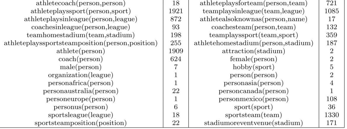
In order to test probabilistic rule learning for facts extracted by NELL, we used the NELL athlete dataset8, which has already been used in the context of meta-interpretive learning of higher-order dyadic Datalog [36]. This dataset contains 10130 facts. The number of facts per predicate is listed in Table 5. The unary predicates in this dataset are deterministic, whereas the binary predicates have a probability attached9.

Table 5: Number of facts per predicate (NELL athlete dataset)

athletecoach(person,person) 18 athleteplaysforteam(person,team) 721 athleteplayssport(person,sport) 1921 teamplaysinleague(team,league) 1085 athleteplaysinleague(person,league) 872 athletealsoknownas(person,name) 17 coachesinleague(person,league) 93 coachesteam(person,team) 132 teamhomestadium(team,stadium) 198 teamplayssport(team,sport) 359 athleteplayssportsteamposition(person,position) 255 athletehomestadium(person,stadium) 187 athlete(person) 1909 attraction(stadium) 2 coach(person) 624 female(person) 2 male(person) 7 hobby(sport) 5 organization(league) 1 person(person) 2 personafrica(person) 1 personasia(person) 4 personaustralia(person) 22 personcanada(person) 1 personeurope(person) 1 personmexico(person) 108 personus(person) 6 sport(sport) 36 sportsleague(league) 18 sportsteam(team) 1330 sportsteamposition(position) 22 stadiumoreventvenue(stadium) 171

Table 5 also shows the types that were used for the variables in the base declarations for the predicates. As indicated in Section 4.5, this typing of the variables forms a syntactic restriction on the possible groundings and ensures that arguments are only instantiated with variables of the appropriate type. Furthermore, the LearnRule function of the ProbFOIL algorithm is based on mFOIL and allows to incorporate a number of variable constraints. To reduce the search space, we imposed that unary predicates that are added to a candidate rule during the learning process can only use variables that have already been introduced. Binary predicates can introduce at most one new variable.

6.2 Relational probabilistic rule learning

In order to illustrate relational probabilistic rule learning with ProbFOIL+ in the context of NELL, we will learn rules and report their respective accuracy for each binary predicate with more then 500 facts. In order to show ProbFOIL+’s speed, also the runtimes are reported. Unless indicated otherwise, both the m-estimate’s m value and the beam width were set to 1. The value of p for rule significance was set to 0.9. The rules are postprocessed such that only range-restricted rules are obtained. Furthermore, to avoid a bias towards to majority class, the examples are balanced, i.e., negative examples are added to balance the number of positives. Anton: negative examples are removed?

8 _{Kindly provided by Tom Mitchell and Jayant Krishnamurthy (CMU).}

athleteplaysforteam

Inducing Probabilistic Logic Programs from Probabilistic Examples? 17

(a) (b)

(c) (d)

Fig. 5: Histogram of probabilities for each of the binary predicates with more then 500 facts: (a) athleteplaysforteam; (b) athleteplayssport; (c) teamplaysinleague; and, (d) athleteplaysinleague.

6.2.1 athleteplaysforteam(person,team)

athleteplaysforteam(A,B) :- coachesteam(A,B).

0.875::athleteplaysforteam(A,B) :- teamhomestadium(B,C), athletehomestadium(A,C).

0.99080::athleteplaysforteam(A,B) :- teamhomestadium(B, ), male(A), athleteplayssport(A, ).

0.75::athleteplaysforteam(A,B) :- teamhomestadium(B, ), athleteplaysinleague(A,C), teamplaysinleague(B,C), athlete(A).

0.75::athleteplaysforteam(A,B) :- teamplayssport(B,C), athleteplayssport(A,C), coach(A), teamplaysinleague(B, ). 0.97555::athleteplaysforteam(A,B) :- personus(A), teamplayssport(B, ).

0.762::athleteplaysforteam(A,B) :- teamplayssport(B,C), athleteplayssport(A,C), personmexico(A), teamplaysinleague(B, ).

0.52571::athleteplaysforteam(A,B) :- teamplayssport(B,C), athleteplayssport(A,C), athleteplaysinleague(A, ), teamplaysinleague(B, ), athlete(A), teamplayssport(B,C).

0.50546::athleteplaysforteam(A,B) :- teamplayssport(B, ), teamplaysinleague(B,C), athleteplaysinleague(A,C), athleteplayssport(A, ).

0.50::athleteplaysforteam(A,B) :- teamplayssport(B, ), teamplaysinleague(B,C), athleteplaysinleague(A,C).

0.52941::athleteplaysforteam(A,B) :- teamplayssport(B, ), teamhomestadium(B, ), coach(A), teamplaysinleague(B, ). 0.55287::athleteplaysforteam(A,B) :- teamplayssport(B, ), teamplaysinleague(B,C), athleteplaysinleague(A,C),

athlete(A).

0.46875::athleteplaysforteam(A,B) :- teamplayssport(B, ), teamplaysinleague(B, ), coach(A), teamhomestadium(B, ).

Dynamics: Evolving Networks

•

Travian

: A massively multiplayer real-time strategy game

•

Commercial game run by TravianGames GmbH

•

~3.000.000 players spread over different “worlds”

•

~25.000 players in one world

[Thon et al., MLJ 11, ECML 08]

World Dynamics

border border border border Alliance 2 Alliance 3 Alliance 4 Alliance 6 P 2 1081 895 1090 1090 1093 1084 1090 915 1081 1040 770 1077 955 1073 804 1054 830 942 1087 786 621 P 3 744 748 559 P 5 861 P 6 950 644 985 932 837 871 777 P 7 946 878 864 913 P 9

Fragment of world with

~10 alliances

~200 players

~600 cities

alliances color-coded

Can we build a model

of this world ?

Can we use it for playing

better ?

[Thon, Landwehr, De Raedt, ECML08]

World Dynamics

border border border border Alliance 2 Alliance 4 Alliance 6 P 2 904 1090 917 770 959 1073 820 762 946 1087 794 632 P 3 761 961 1061 607 988 771 924 583 P 5 951 935 948 938 867 P 6 950 644 985 888 844 875 783 P 7 946 878 864 913

Fragment of world with

~10 alliances

~200 players

~600 cities

alliances color-coded

Can we build a model

of this world ?

Can we use it for playing

better ?

[Thon, Landwehr, De Raedt, ECML08]

World Dynamics

border border border border Alliance 2 Alliance 4 Alliance 6 P 2 918 1090 931 779 977 835 781 958 1087 808 701 P 3 838 947 1026 1081 833 1002 987 827 994 663 P 5 1032 1026 1024 1049 905 926 P 6 986 712 985 920 877 807 P 7 895 959 P 10 824

Fragment of world with

~10 alliances

~200 players

~600 cities

alliances color-coded

Can we build a model

of this world ?

Can we use it for playing

better ?

[Thon, Landwehr, De Raedt, ECML08]

Causal Probabilistic

Time-Logic (CPT-L)

[Thon et al, MLJ 11]

how does the

world change

over time?

0.4::conquest(Attacker,C); 0.6::nil <- 





city(C,Owner),city(C2,Attacker),close(C,C2).

if

cause

holds at time T

one of the

effects

holds at time T+1

Limitations CPT-L

Inference slow / scalability

•

uses knowledge compilation method

•

compile formula for

•

exponential in number of time steps

No continuous distributions

•

needed for robotics / relational tracking

applications

Relational

Tracking

•

Track people or objects

over time? Even if

temporarily hidden?

•

Recognize activities?

•

Infer object properties?

Fig. 4. Tracking results from experiment 2. In frame 5, two groups are present. In frame 15, the tracker has correctly split group 1 into 1-0 and 1-1 (see Fig. 3). Between frames 15 and 29, group 1-0 has split up into groups 1-0-0 and 1-0-1, and split up again. New groups, labeled 2 and 3, enter the field of view in frames 21 and 42 respectively.

Six frames of the current best hypothesis from experiment 2 are shown in Fig. 4, the corresponding hypothesis tree is shown in Fig. 3. The sequence exemplifies movement and formation of several groups.

A. Clustering Error

Given the ground truth information on a per-beam basis we can compute the clustering error of the tracker. This is done

by counting how often a track’s set of points _P contains too

many or wrong points (undersegmentation) and how often _P

is missing points (oversegmentation) compared to the ground truth. Two examples for oversegmentation errors can be seen in Fig. 4, where group 0 and group 1-0 are temporarily oversegmented. However, from the history of group splits and merges stored in the group labels, the correct group

0 0.1 0.2 0.3 0.4 0.5 0.6 0.5 1 1.5 2 2.5 3 3.5

Error rates per track and frame

Clustering distance threshold d_P (m)

w/o tracking Overs. + Unders. Oversegm. Undersegm. 0 0.2 0.4 0.6 0.8 1 0 4 8 12 16 20

Avg. cycle time (sec)

Number of people in ground truth Group tracker

People tracker

Fig. 5. Left: clustering error of the group tracker compared to a memory-less single linkage clustering (without tracking). The smallest error is achieved for a cluster distance of 1.3 m which is very close to the border of personal and social space according to the proxemics theory, marked at 1.2 m by the vertical line. Right: average cycle time for the group tracker versus a tracker for individual people plotted against the ground truth number of people.

relations can be determined in such cases.

For experiment 1, the resulting percentages of incorrectly clustered tracks for the cases undersegmentation, overseg-mentation and the sum of both are shown in Fig. 5 (left),

plotted against the clustering distance dP . The figure also

shows the error of a single-linkage clustering of the range data as described in section II. This implements a memory-less group clustering approach against which we compare the clustering performance of our group tracker.

The minimum clustering error of 3.1% is achieved by the

tracker at dP = 1.3 m. The minimum error for the

memory-less clustering is 7.0%, more than twice as high. In the more complex experiment 2, the minimum clustering error of the tracker rises to 9.6% while the error of the memory-less clustering reaches 20.2%. The result shows that the

group tracking problem is a recursive clustering problem that

requires integration of information over time. This occurs when two groups approach each other and pass from opposite directions. The memory-less approach would merge them immediately while the tracking approach, accounting for the velocity information, correctly keeps the groups apart.

In the light of the proxemics theory the result of a minimal clustering error at 1.3 m is noteworthy. The theory predicts that when people interact with friends, they maintain a range of distances between 45 to 120 cm called personal space. When engaged in interaction with strangers, this distance is larger. As our data contains students who tend to know each other well, the result appears consistent with Hall’s findings.

B. Tracking Efficiency

When tracking groups of people rather than individuals, the assignment problems in the data association stage are of course smaller. On the other hand, the introduction of an additional tree level on which different models hypoth-esize over different group formation processes comes with additional computational costs. We therefore compare our system with a person-only tracker which is implemented by inhibiting all split and merge operations and reducing the

cluster distance dP to the very value that yields the lowest

error for clustering single people given the ground truth. For

Box scenario

•

object tracking even

when invisible

•

estimate spatial relations

Relational State Estimation

over Time

80 [Nitti et al, IROS 13]

Magnetism scenario

•

object tracking

•

category estimation

81

82

Magnetic scenario

●

3 object types: magnetic, ferromagnetic, nonmagnetic

●

Nonmagnetic objects do not interact

●

A magnet and a ferromagnetic object attract each other

●

Magnetic force that depends on the distance

84

DC Particle Filter (DCPF)

Dynamic Distributional Clauses

DCPF

Particle Filter

Flexible (relational) state representation

Fast inference (state estimation) in general models

Goal

“A particle filter for hybrid relational domains” IROS 2013


D. Nitti, T. De Laet, L. De Raedt

Dynamic Distributional

Clauses

Prior distribution p(x

₀

)

State transition model p(x

_t

|x

_t-1,

u

_t

)

Measurement model p(z

_t

|x

_t

)

Other rules: p(x’

_t

|x’'

_t

)

21

Dynamic Distributional Clauses

hidden state

observation time

u

_t-1

u

_t

actions

●

Prior distribution p(x

0

) or p(x

1

|z

1

)

●

State transition model p(x

t

|x

t-1

,u

t

)

●

Measurement model p(z

t

|x

t

)

●

Other rules: p(x'

86

Magnetic scenario

●

3 object types: magnetic, ferromagnetic, nonmagnetic

●

2 magnets attract or repulse




●

Next position after attraction

type(X)

_t

~ finite([1/3:magnet,1/3:ferromagnetic,1/3:nonmagnetic])

←

object(X).

interaction(A,B)

_t

~ finite([0.5:attraction,0.5:repulsion])

←




object(A), object(B), A<B,type(A)

_t

= magnet,type(B)

_t

= magnet.

pos(A)

_t+1

~ gaussian(middlepoint(A,B)

_t

,Cov)

←




near(A,B)

_t

, not(held(A)), not(held(B)),




interaction(A,B)

_t

= attr,

c/dist(A,B)

_t2

_{> friction(A)}

t

.

88

Classical Particle Filter vs DCPF

●

Classical PF

–

Fixed set of random variables

–

Update the entire state

●

DCPF

–

Adaptive state

(particle): the number of facts / sampled

random variables can change over time

–

Particles are partial interpretations

–

Expressive language

1.1
 2.3 10.3 1.2
 2.1
 10.5

x

_t+1

(i)

x

_t

(i) Pos(1)=(0, 3) Pos(2)=(0, 1) right(X,Y) near(X,Y)
 interaction(X,Y) type(X) ~ [1/3:magnet,...] [...]

89

Optimized inference: partial state

Pos(1)=(0, 3) Pos(2)=(0, 1) right(X,Y) near(X,Y)
 interaction(X,Y) type(X) ~ [1/3:magnet,...] [...] Pos(1)=(0, 2) Pos(2)=(0, 1) near(1,2)=true type(1)=nonmagnetic right(X,Y) near(X,Y)
 interaction(X,Y) type(X) ~ [1/3:magnet,...] [...] Pos(1)=(0, 3) Pos(2)=(0, 1) near(1,2)=false
 near(2,1)=false
 interaction(1,2)=none type(1)=nonmagnetic type(2)=nonmagnetic [...] Pos(1)=(0, 2) Pos(2)=(0, 1) near(1,2)=true
 near(2,1)=true
 interaction(1,2)=none type(1)=nonmagnetic type(2)=nonmagnetic [...]

Classical particle filter

Distributional Clauses Particle Filter (DCPF)

Sampled

Inference in DCPF

Two steps:

Query p(z

_t+1

|x

_t+1

) (weighting + part of sampling step)

Query p(x

_t+1|

x

t

, u

t+1

) (to complete the sampling step)

using the DC inference

particles are partial interpretations

bel(x

t

) fully represented by {x

t(i)

}

∪

Program

History {x

0:t-1(i)

} not necessary

91

Experiments

●

Particles are partial state, remaining variables are

marginalized

Ongoing Work

•

Online parameter learning [Nitti, ICRA 2014]

•

Integrate with planning [Nitti, ECML

15,EWRL 15]

•

Applications in robotics (also to learn

affordances)

Learning relational affordances

Learn probabilistic model

From two object interactions

Generalize to N

Shelf push Shelf tap Shelf grasp

Moldovan et al. ICRA 12, 13, 14

Occluded Object

Search

94

•

Models of objects and their spatial arrangement

•

different types of objects suitable for different tasks

•

shelves with objects of different shape and size

•

given a task, find an object to perform that task

ProbLog  for  ac+vity  recogni+on  from  video

 

 

Thanks!

http://dtai.cs.kuleuven.be/problog

Vaishak Belle Maurice Bruynooghe Bart Demoen Anton Dries Daan Fierens Jason Filippou Bernd Gutmann Manfred Jaeger Gerda Janssens Kristian Kersting Angelika Kimmig Theofrastos Mantadelis Wannes Meert Bogdan Moldovan Siegfried Nijssen Davide Nitti Joris Renkens Kate Revoredo Ricardo Rocha Vitor Santos Costa Dimitar Shterionov

Ingo Thon Hannu Toivonen

Guy Van den Broeck

Mathias Verbeke

Jonas Vlasselaer ₉₆

•

PRISM

http://sato-www.cs.titech.ac.jp/prism/

•

ProbLog2

http://dtai.cs.kuleuven.be/problog/

•

Yap Prolog http://www.dcc.fc.up.pt/~vsc/Yap/ includes

•

ProbLog1

•

cplint

https://sites.google.com/a/unife.it/ml/cplint

•

CLP(BN)

•

LP2

•

PITA

in XSB Prolog http://xsb.sourceforge.net/

•

AILog2

http://artint.info/code/ailog/ailog2.html 

•

SLPs

http://stoics.org.uk/~nicos/sware/pepl

•

contdist

http://www.cs.sunysb.edu/~cram/contdist/

•

DC

https://code.google.com/p/distributional-clauses

•

WFOMC

http://dtai.cs.kuleuven.be/ml/systems/wfomc

PLP

Systems

97

1

References

Bach SH, Broecheler M, Getoor L, O’Leary DP (2012) Scaling MPE inference for constrained continuous Markov random fields with consensus optimization. In: Proceedings of the 26th Annual Conference on Neural Information Processing Systems (NIPS-12)

Broecheler M, Mihalkova L, Getoor L (2010) Probabilistic similarity logic. In: Pro-ceedings of the 26th Conference on Uncertainty in Artificial Intelligence (UAI-10)

Bryant RE (1986) Graph-based algorithms for Boolean function manipulation. IEEE Transactions on Computers 35(8):677–691

Cohen SB, Simmons RJ, Smith NA (2008) Dynamic programming algorithms as products of weighted logic programs. In: Proceedings of the 24th International Conference on Logic Programming (ICLP-08)

Cussens J (2001) Parameter estimation in stochastic logic programs. Machine Learning 44(3):245–271

De Maeyer D, Renkens J, Cloots L, De Raedt L, Marchal K (2013) Phenetic: network-based interpretation of unstructured gene lists in e. coli. Molecular BioSystems 9(7):1594–1603

De Raedt L, Kimmig A (2013) Probabilistic programming concepts. CoRR abs/1312.4328

De Raedt L, Kimmig A, Toivonen H (2007) ProbLog: A probabilistic Prolog and its application in link discovery. In: Proceedings of the 20th International Joint Conference on Artificial Intelligence (IJCAI-07)

De Raedt L, Frasconi P, Kersting K, Muggleton S (eds) (2008) Probabilistic Induc-tive Logic Programming — Theory and Applications, Lecture Notes in Artificial Intelligence, vol 4911. Springer

Eisner J, Goldlust E, Smith N (2005) Compiling Comp Ling: Weighted dynamic programming and the Dyna language. In: Proceedings of the Human Language Technology Conference and Conference on Empirical Methods in Natural Lan-guage Processing (HLT/EMNLP-05)

Fierens D, Blockeel H, Bruynooghe M, Ramon J (2005) Logical Bayesian networks and their relation to other probabilistic logical models. In: Proceedings of the 15th International Conference on Inductive Logic Programming (ILP-05) Fierens D, Van den Broeck G, Bruynooghe M, De Raedt L (2012) Constraints

for probabilistic logic programming. In: Proceedings of the NIPS Probabilistic Programming Workshop

Fierens D, Van den Broeck G, Renkens J, Shterionov D, Gutmann B, Thon I, Janssens G, De Raedt L (2014) Inference and learning in probabilistic logic programs using weighted Boolean formulas. Theory and Practice of Logic Pro-gramming (TPLP) FirstView

Getoor L, Friedman N, Koller D, Pfe↵er A, Taskar B (2007) Probabilistic relational models. In: Getoor L, Taskar B (eds) An Introduction to Statistical Relational Learning, MIT Press, pp 129–174

Goodman N, Mansinghka VK, Roy DM, Bonawitz K, Tenenbaum JB (2008) Church: a language for generative models. In: Proceedings of the 24th Con-ference on Uncertainty in Artificial Intelligence (UAI-08)

Gutmann B, Thon I, De Raedt L (2011a) Learning the parameters of probabilis-tic logic programs from interpretations. In: Proceedings of the 22nd European

2

Conference on Machine Learning (ECML-11)

Gutmann B, Thon I, Kimmig A, Bruynooghe M, De Raedt L (2011b) The magic of logical inference in probabilistic programming. Theory and Practice of Logic Programming (TPLP) 11((4–5)):663–680

Huang B, Kimmig A, Getoor L, Golbeck J (2013) A flexible framework for prob-abilistic models of social trust. In: Proceedings of the International Conference on Social Computing, Behavioral-Cultural Modeling, and Prediction (SBP-13)

Jaeger M (2002) Relational Bayesian networks: A survey. Link¨oping Electronic

Articles in Computer and Information Science 7(015)

Kersting K, Raedt LD (2001) Bayesian logic programs. CoRR cs.AI/0111058 Kimmig A, Van den Broeck G, De Raedt L (2011a) An algebraic Prolog for

rea-soning about possible worlds. In: Proceedings of the 25th AAAI Conference on Artificial Intelligence (AAAI-11)

Kimmig A, Demoen B, De Raedt L, Santos Costa V, Rocha R (2011b) On the im-plementation of the probabilistic logic programming language ProbLog. Theory and Practice of Logic Programming (TPLP) 11:235–262

Koller D, Pfe↵er A (1998) Probabilistic frame-based systems. In: Proceedings of

the 15th National Conference on Artificial Intelligence (AAAI-98)

McCallum A, Schultz K, Singh S (2009) FACTORIE: Probabilistic programming via imperatively defined factor graphs. In: Proceedings of the 23rd Annual Con-ference on Neural Information Processing Systems (NIPS-09)

Milch B, Marthi B, Russell SJ, Sontag D, Ong DL, Kolobov A (2005) Blog: Proba-bilistic models with unknown objects. In: Proceedings of the 19th International Joint Conference on Artificial Intelligence (IJCAI-05)

Moldovan B, De Raedt L (2014) Occluded object search by relational a↵ordances.

In: IEEE International Conference on Robotics and Automation (ICRA-14) Moldovan B, Moreno P, van Otterlo M, Santos-Victor J, De Raedt L (2012)

Learn-ing relational a↵ordance models for robots in multi-object manipulation tasks.

In: IEEE International Conference on Robotics and Automation (ICRA-12) Muggleton S (1996) Stochastic logic programs. In: De Raedt L (ed) Advances in

Inductive Logic Programming, IOS Press, pp 254–264

Nitti D, De Laet T, De Raedt L (2013) A particle filter for hybrid relational do-mains. In: Proceedings of the IEEE/RSJ International Conference on Intelligent Robots and Systems (IROS-13)

Nitti D, De Laet T, De Raedt L (2014) Relational object tracking and learning. In: IEEE International Conference on Robotics and Automation (ICRA), June 2014

Pfe↵er A (2001) IBAL: A probabilistic rational programming language. In:

Pro-ceedings of the 17th International Joint Conference on Artificial Intelligence (IJCAI-01)

Pfe↵er A (2009) Figaro: An object-oriented probabilistic programming language.

Tech. rep., Charles River Analytics

Poole D (2003) First-order probabilistic inference. In: Proceedings of the 18th International Joint Conference on Artificial Intelligence (IJCAI-03)

Richardson M, Domingos P (2006) Markov logic networks. Machine Learning 62(1-2):107–136

Santos Costa V, Page D, Cussens J (2008) CLP(BN): Constraint logic

3

Sato T (1995) A statistical learning method for logic programs with distribution semantics. In: Proceedings of the 12th International Conference on Logic Pro-gramming (ICLP-95)

Sato T, Kameya Y (2001) Parameter learning of logic programs for symbolic-statistical modeling. J Artif Intell Res (JAIR) 15:391–454

Sato T, Kameya Y (2008) New advances in logic-based probabilistic modeling by prism. In: Probabilistic Inductive Logic Programming, pp 118–155

Skarlatidis A, Artikis A, Filiopou J, Paliouras G (2014) A probabilistic logic pro-gramming event calculus. Theory and Practice of Logic Propro-gramming (TPLP) FirstView

Suciu D, Olteanu D, R´e C, Koch C (2011) Probabilistic Databases. Synthesis Lectures on Data Management, Morgan & Claypool Publishers

Taskar B, Abbeel P, Koller D (2002) Discriminative probabilistic models for rela-tional data. In: Proceedings of the 18th Conference on Uncertainty in Artificial Intelligence (UAI-02)

Thon I, Landwehr N, De Raedt L (2008) A simple model for sequences of rela-tional state descriptions. In: Proceedings of the European Conference on Ma-chine Learning and Knowledge Discovery in Databases (ECML/PKDD-08)

Thon I, Landwehr N, De Raedt L (2011) Stochastic relational processes: Efficient

inference and applications. Machine Learning 82(2):239–272

Van den Broeck G, Thon I, van Otterlo M, De Raedt L (2010) DTProbLog: A decision-theoretic probabilistic Prolog. In: Proceedings of the 24th AAAI Con-ference on Artificial Intelligence (AAAI-10)

Van den Broeck G, Taghipour N, Meert W, Davis J, De Raedt L (2011) Lifted probabilistic inference by first-order knowledge compilation. In: Proceedings of the 22nd International Joint Conference on Artificial Intelligence (IJCAI-11) Vennekens J, Verbaeten S, Bruynooghe M (2004) Logic programs with annotated

disjunctions. In: Proceedings of the 20th International Conference on Logic Pro-gramming (ICLP-04)

Vennekens J, Denecker M, Bruynooghe M (2009) CP-logic: A language of causal probabilistic events and its relation to logic programming. Theory and Practice of Logic Programming (TPLP) 9(3):245–308

Wang WY, Mazaitis K, Cohen WW (2013) Programming with personalized pager-ank: a locally groundable first-order probabilistic logic. In: Proceedings of the 22nd ACM International Conference on Information and Knowledge Manage-ment (CIKM-13)