Weighted Heuristic Ensemble of Filters

Weighted Heuristic Ensemble of Filters

Ghadah Aldehim

School of Computing Sciences University of East Anglia

Norwich, NR4 7TJ, UK G.Aldehim@uea.ac.uk

Wenjia Wang

University of East Anglia Norwich, NR4 7TJ, UK Wenjia.Wang@uea.ac.uk Abstract—Feature selection has become increasingly

important in data mining in recent years due to the rapid increase in the dimensionality of big data. However, the reliability and consistency of feature selection methods (filters) vary considerably on different data and no single filter performs consistently well under various conditions. Therefore, feature selection ensemble has been investigated recently to provide more reliable and effective results than any individual one but all the existing feature selection ensemble treat the feature selection methods equally regardless of their performance. In this paper, we present a novel framework which applies weighted feature selection ensemble through proposing a systemic way of adding different weights to the feature selection methods-filters. Also, we investigate how to determine the appropriate weight for each filter in an ensemble. Experiments based on ten benchmark datasets show that theoretically and intuitively adding more weight to ‘good filters’ should lead to better results but in reality it is very uncertain. This assumption was found to be correct for some examples in our experiment. However, for other situations, filters which had been assumed to perform well showed bad performance leading to even worse results. Therefore adding weight to filters might not achieve much in accuracy terms, in addition to increasing complexity, time consumption and clearly decreasing the stability.

Keywords—Feature selection; Ensemble; Classification; stability; Heuristics; Weight

I. INTRODUCTION

Ensemble ranking of features is the problem of aggregating different ranks to improve the performance of the feature selection. There are two types of rank aggregation: unsupervised and supervised. Most of the unsupervised rank aggregation methods implicitly conduct majority voting to construct the final rank [1]. For instance, mean rank aggregation computes the mean of the ranks of the features selected by the ranking filters. However, the main concern with these methods is that they treat all the feature selection (FS) methods equally regardless of their performance.

On the other hand, supervised rank aggregation usually determines the weights of each ranking list by learning an aggregation function using training data [2, 3]. For example, in a meta-analytic bioinformatics study some labs are more efficient in data collection and analyzing procedure than other labs; also, in a meta-search study more capacity and accuracy could be found while using some search engines than others. The success of supervised rank aggregation in other applications provides the main motivation for applying supervised rank aggregation in ensemble feature selection. Our

hypothesis is that the members in an ensemble - filters, should be weight differently based on their performance.

In this paper, we will investigate how to determine the appropriate weight for each filter in an ensemble. To the best of my knowledge, so far this is the first study that gives weight to some filter methods based on validation set or by using prior-knowledge when aggregating the output of the filters in the ensemble.

The rest of this paper is organized as follows: Section 2 presents related work. Section 3 describes the frameworks of adding fixed weight, variable weight and selective filters. Section 4 gives the results and evaluates the three proposed approaches. Section 5 presents the broad dissection and evaluation of the experiments. Finally, Section 6 draws conclusions from our work.

II. RELATED WORK

The rank aggregation technique has been investigated and used in many application areas, such as metasearch, image fusion and many others. Aslam and Montague [4] proposed two algorithms based on Borda Count for metasearch, namely Borda-fuse and Weighted Borda-fuse. Borda-fuse gives the same weight to all engines, whereas Weighted Borda-fuse uses different weights. It is an earlier study that gives different base rankers different weights by using labelled training data. For instance, the weights can be determined by using the MAP (Mean Average Precision) of the base rankers. So, in order to determine the precision value of each engine, training data is required by Weighted Borda-fuse.

While, training details not required by Borda-fuse, rank results can be directly unified by base rankers score. It has been observed from experimental results that Weighted Borda-fuse is indeed superior to fuse. However, Weighted Borda-fuse has got the problem of calculating the weights of the ranking list independently by using heuristics. It is also unclear whether the same concept can be applied to other methods [2]. The authors themselves pointed out that it may not always be optimal to use precision values as weight. The ideal condition would be to fine tune the weight vector used by the Borda Count by means of certain techniques. The results will reveal the potency of using precision values as weights. Also, another limitation of Borda Count and Weighted Borda-fuse model is that there is no clear way of handling missing documents[5].

Liu et al. [2] deal with supervised rank aggregation (SRA). In their procedure, training data is provided in the form of true relative ranks of some entities and the weights are optimized

November 10-11, 2015 | London, UK with the support of the training data as well as the aggregated

list; instead of pre-specified constants, generally the weights are treated as parameters in these models. Unavailability of any training data in many applications is a problem of SRA.

In the biomedical applications of computational biology, Abeel et al. [6] discussed the robustness of ensemble feature selection by using embedded method, support vector machine - recursive feature elimination (SVM-RFE), then obtaining different rankings by bootstrapping the training data. They used two aggregation methods: complete linear aggregation and complete weight linear aggregation. The complete linear aggregation uses the complete ranking of all the features to produce the ensemble result by summing the ranks, over all bootstrap samples and setting all weights equal to one. While, the complete weight linear aggregation measures weights of the scores of each bootstrap ranking by using AUC.

Although greater accuracy can be achieved by supervised aggregation, the labelled data are not always available in practice [1]. Also, a prudent way of handling the quality difference is assigning weights to base rankers; in practice, designing a proper weight specification scheme can be rather difficult, especially when availability of prior knowledge on base rankers is poor [7].

Based on the above studies we noted that ensemble filters is similar to order rank aggregation in metasearch. Therefore, in this research the methods proposed for metasearch will be investigated with an attempt to improve the results of ensemble feature selection.

III. WEIGHTED HEURISTIC ENSEMBLE OF FILTERS

Intuitively speaking, it is reasonable that the filters should be treated differently in accordance with their performance, as in reality, there are some differences in the performances of filters. Thus, the use of different weights for calculating the total scores of the selected features may improve the performance. Therefore, in this section, three methods are proposed: the first one assigns fixed weight to some filters, the second one assigns variable weights to some filters in order to investigate the impact of weighted filters on the final resultof the ensemble aggregation. And, the third one assigns weight equal to one to some filters and assigns weight equal to zero to other filters, which means, in other words, it selects some filters and discards others based on the training set.

We first give some definitions and notations. Given a set of features X, let be a subset of X and assume that there is a ranking order among the features in . Consider an ensemble consisting of filters, then we assume each filter provides a

feature ranking = { }, all the rankings are

aggregated into a consensus feature ranking by a weighted voting function.

∑ (1)

Where, E( ) is the aggregating function of an ensemble,

denotes a weight function. If we assume that all of the filters

are equally important then set for i=1, ..., , then as in our previous paper about Heuristic

Ensemble of Filters (HEF) [8]

By assigning different weight values to different filters, filter with large weight should play a more important role in

generating the consensus feature ranks. A. Fixed Weight Methods (FWHEF)

In this section, we give more weight to subset filters (SF) and less weight to rank filters (RF) in order to allow SF play more important role in generating the consensus feature ranks. The reason for adding more weight to SF is that many SF methods have been demonstrated to be efficient in removing both irrelevant and redundant features. In such SF methods, the existence and effect of redundant features are also taken into account to approximate the optimal subset [9-11]. Whereas, RF methods are not designed for removing redundant features because they evaluate each feature individually. However, how to decide the appropriate weights to SF and RF is not an easy task. Because no prior knowledge on filters is available, no training sets can be used, so we select different values as a weight in the following systematic manner:

∑ (2) S.T. ∑ = 1 (3)

Where E1, is the aggregating function of FWHEF and each filter is assigned a weight , where is the same as that in

(1).

{

(4)

Where is coefficient generated to give more weight to the feature selected by SF, and is another coefficient generated to give less weight to the feature selected by RF, and the sum of these two coefficients equal to one. We start with , then add

each by ∆β and so on, and also start with , then add

each add by ∆λ and so on, as follow:

∆β (5) ∆λ (6)

The values for and could be determined based on the performance of FWHEF. However, because of the space limitation we select in this paper just one case which set β=0.35 and λ=0.15.

B. Variable Weight Based on Validation Set (VWHEF) In this section, we discuss how to apply variable weight on some filters based on the classification accuracy. By assuming that if a filter produces high accuracy it means it can select more relevant and important features and vice versa by using the same classifier. Variable Weighted HEF (VWHEF) uses the classification accuracy values to compute the weights of each filter, so a training set is required. Fig.1 illustrates how the training data was split into training and validation set in order to evaluate the accuracy for each of the individual filters. The experiments were performed through 10-fold cross validation. We split the training set into ten subsets, used 9-folds for training and 1-fold for validation, then rotated this process ten times to create ten data sets. Then we took the average classification accuracy over the ten validation sets as the final results of each filter.

This process is repeated in each fold of the external 10-fold cross validations which evaluate the VWHEF by using a test set after adding different weight to some filters, as seen in fig. 2. Since we cannot use the test set to determine which filters have the higher accuracy to give them more weight and the reason for that is to avoid the bias, we use the validation set to estimate accuracy on the test set. Also, we take the average accuracy of ten validation sets to produce more relible results than using just one validation set.

1) Variance based Weight Estimation:

We design a heuristic method to compute the weight based on the classification accuracy and variance on the validation set, because there are no standard methods to compute the weight. Aslam and Montague [4] mentioned that it may not always be optimal to use classification precision values as weight [12]. Accordingly, in order to calculate the weight of each filter in VWHEF, we need to find values which have a relation with the accuracy from each filter, giving more weight to filters with high accuracy and low weight to filters with low accuracy. Note that the weights based on classification accuracy range between 100 and 0 which is not the perfect way to use this accuracy directly as weight.

Fig. 1. Determining the weight by classification accuracy on validation data set

Fig. 2. Framework of Variable Weight Based on Validation Set

PROCEDURE 1: COMPUTE THE WEIGHT FOR VWHEF

1. Rank all filters ( ) based on the final average accuracy of validation set.

2. Compute σ between the final accuracy of each filters ( ) 3. = σ , If σ < 1 then = σ+1 4. ∑ 5. For i = 2 to 6. Compute diff - ). 7. = , if < 1 then = 1 8. ∑ 9. i = i+1

10. Go back to the loop

Thus, we use standard deviation σ between the average accuracy of each filter as a measure to evaluate how far the accuracy of these filters differs. If σ is high this means that there are big accuracy differences between the filters, which is a motivation to give high weight to the highest filter accuracies and vice versa. If σ is low, this means there are small accuracy differences, or in other words all filters produce similar results and there is no need to give high weight to the highest filter accuracy. So, based on this justification we use σ as a weight value to the highest filter accuracy. With the same idea, we compute the weight of the second higher accuracy filter, but this time we want the second weight to become smaller than the first one. Therefore, we first measure the difference between the highest filter accuracy and the second one, and then take off this difference from the σ, but if the second weight becomes less than 1 then the weight will be 1. The remaining filters have the similar way to determine the weight as the second filter. The framework to compute the weight is illustrated in Procedure 1 above.

C. Selective Filters Based on Validation Set (SFHEF) When we assume that a filter is able to select more relevant and important features, this should lead to producing a high accuracy result and on the other hand if a filter is unable to select relevant and important features, this should lead to producing a lower accuracy results by using same classifier. This assumption motivates us to ignore the features selected by the worst performing filters and just to focus on the features selected by the best filters by aggregating their features.

In this section, as our experiment was provided with an ensemble of five filters, we select the top two filters only, based on their accuracy, to aggregate their results selected by their features and disregard the results of the three remaining filters. In this case SFHEF can be a special case of VWHEF as we can set and . By using this method, we still need to use training sets to rank the filter based on their accuracy then we aggregate the features selected by the two top filters. Thus, we use the same framework as in Fig.1 but with weight equal one for the first two filters and weight equal to zero for the remaining filters. The aims of using this method are to improve the feature selected results by SFHEF and decrease the number of features aggregated by SFHEF in addition to improving the accuracy and stability.

November 10-11, 2015 | London, UK IV. EXPERIMENTS

A. Data

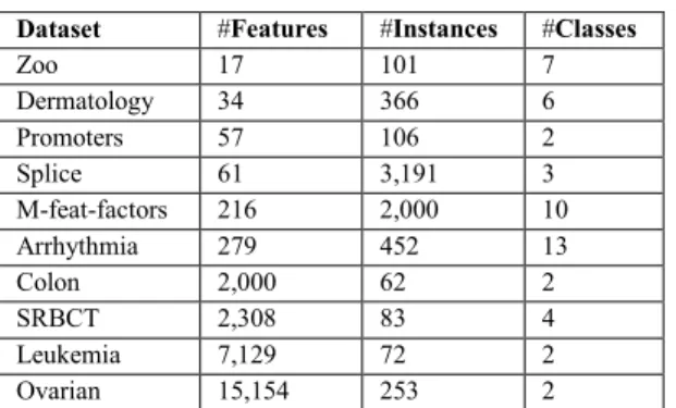
Ten benchmark datasets from different domains are used in our experiments to test the performance of our three proposed weighted heuristic ensemble of filters. Six of them, Zoo, Dermatology, Promoters, Splice, Multi-feature-factors and Arrhythmia, are from the UCI Machine Learning Repository,1 two others (Colon and Leukaemia) from the Bioinformatics Research Group2_{, and the final three (SRBCT, Leukemia and} Ovarian) from the Microarray Datasets website.3

TABLE I. DESCRIPTION OF DATASETS

Dataset #Features #Instances #Classes

Zoo 17 101 7 Dermatology 34 366 6 Promoters 57 106 2 Splice 61 3,191 3 M-feat-factors 216 2,000 10 Arrhythmia 279 452 13 Colon 2,000 62 2 SRBCT 2,308 83 4 Leukemia 7,129 72 2 Ovarian 15,154 253 2

B. Experimental Design Procedure and Evaluation methods To verify the consistency of the feature selection methods, in our experiments, we used three types of classifiers: NBC (Naive Bayesian Classifier) [13], KNN (k-Nearest Neighbor) [14] and SVM (Support Vector Machine) [15]. These three algorithms were chosen because they represent three quite different approaches in machine learning and they are state-of-the-art algorithms that are commonly used in data mining practice. Also, we applied five filters as members in the ensemble: 2 SF (FCBF and CFS) and 3 RF (ReliefF, GR and chi- as seen in fig. 2. The heuristic ensemble of filters (HEF) starts by running SF and RF. After that, a consensus number of features selected by SF is taken as a cut-off point for the rankings generated by RF. By running this heuristic step, we can obtain quick answers for cutting off the number of features in the ranker, which will accelerate the ensemble algorithm. Therefore, we will not need to select various feature numbers to test the performance.

Ambroise and McLachlan [16] recommend using 10-fold rather than leave-one-out cross-validation, because the latter one can be highly variable. In each fold, we firstly ran all FS methods (FCBF, CFS, ReliefF, Gain Ratio and Chi- ) by using 90% of all the instances (9 folds), after that the subsets produced by each FS were weighed based on each of the techniques we used (FWHEF, VWHEF and SFHEF) to generate the ensemble results and produce subsets of ranked feature. Then we used these rank subsets as input to the classifier with the same 90% of instances (9 folds). Following this, the accuracy of this subset was estimated over the unseen 10% of the data (1 fold). This was performed 10 times, each time proposing a possible different feature subset. In this way,

1_{http://repository.seasr.org/Datasets/UCI/arff/}

2 _{http://www.upo.es/eps/aguilar/datasets.html} 3 _{http://csse.szu.edu.cn/staff/zhuzx/Datasets.html}

estimated accuracies and selected attribute numbers, which were the results of a mean over 10 ‘cross-validation samples’. Each experiment was then repeated ten times with differently shuffled random seeds in order to assess the consistency and reliability of the results. In total, 51,000 models (17 (5 FS + 12 ensemble) 10 (data sets) 3 (classifiers) 10 (run) 10 (folds)) were built for the experiments.

The statistical significance of the results of the multiple runs for each experiment was calculated, and the comparisons between accuracies were carried out with a non-parametric Friedman test with a significance level of 0.05 [17]. It ranks the algorithms for each data set independently, the best performance algorithm getting the rank of 1, the second best rank 2, and so on. In case of ties, average ranks are assigned. Then, if the null hypothesis is rejected, the Nemenyi test can proceed. It is used when all algorithms are compared to each other on multiple testing datasets. The performance of two algorithms is significantly different if the corresponding average ranks differ by at least the critical difference:

CD= √ (7)

Where A is the number of algorithms, D, number of data sets used and critical value which determined on the

Studentized range statistic divided by √ [17].

Moreover, in addition to accuracy, we will measure the stability of FS, as in each fold the FS method may produce different feature subsets. Measuring stability requires a similarity measure for the FS results. The stability measure used in our investigation is Average Tanimoto Index (ATI) [18], as the subset cardinality is not equal in our research. ATI evaluates pair-wise similarities between subsets in the system (10 folds).

V. RESULTS

In this section, the classification accuracy and stability results obtained after applying the different proposed ensembles were shown. To sum up, three ensemble approaches were tested: FWHEF VWHEF and SFHEF. Also, we compared these three ensemble approaches with the simple HEF which treats all filter members equally to demonstrate the capability of the proposed ensemble approaches to improve the results.

A. Accuracy Evaluation with Different Classifiers

This section showed the accuracy of results obtained with NB, KNN and SVM. Simple HEF and three proposed ensembles were used over 10 datasets with all the features selected by 5 filters and the top 75%, 50% and 25% of the selected features. It should be noticed that the features selected by HEF, FWHEF, VWHEF are the union of the features selected by each one of the filters, but with different ranking.

Therefore, we found that the accuracy of HEF, FWHEF, VWHEF with all features selected had the same accuracy because the same features had been selected for them. While, SFHEF had different accuracy because the features that were selected had been aggregated from only two filters with high accuracy, the selected features were different.

Fig. 3. The average test accuracy of NB by using 10 datasets focusing on different methods

Fig. 4. The average test accuracy of KNN by using 10 datasets focusing on different methods

Fig. 5. The average test accuracy of NB by using 10 datasets focusing on different methods

Figures 3, 4 and 5 showed the average test accuracy of NB, KNN and SVM classifiers respectively by using 10 datasets focusing on different methods. It is clearly seen that the classification accuracy using the top 75% of the selected features produced highest accuracy in the three classifiers because the irrelevant and redundant features which could have lowered the score had been removed. While, the classification accuracy using only the top 25% of the selected features produced lowest accuracy, because some relevant and important features which had median scores were removed and just the top 25% of the features were used. As a result, heuristically using the top 75% of the selected features was the best choice to select and concentrate on.

On the other hand, focusing on the ensemble approaches, SFHEF-75% had the highest accuracy by NB. In contrast, it was the lowest one when using only 25% of the selected features with all classifiers. While FWHEF-50% had the highest accuracy by KNN and VWHEF-75% had the highest accuracy by SVM. However, the ensemble approaches produced different accuracy when using different classifiers. So, no particular preferences were given to one over the others which was proved statistically by the Nemenyi test. The difference between the four ensemble approaches with all classifiers was not significant, except SVM with 25% features selected, as we can see in figure 6.

Fig. 6. The average test accuracy of SVM by using 10 datasets focusing on different methods

We can identify two groups of ensemble approaches: the performance of SFHEF-25 is significantly worse than that of FWHEF-25. The statistical statement would be that the experimental results are not sufficient to reach any conclusion regarding VWHEF-25 and HEF-25 which belong to both groups.

In the next section, whether the proposed ensemble approaches were stable and to what extent they remained more stable than the simple HEF has been analyzed.

B. Stability Evaluation

In practice, high stability of feature selection is equally important as high classification accuracy [19]. Numerous feature selection algorithms have been proposed; however, if we repeat the feature selection process by slightly changing the data, these algorithms do not inevitably identify the same candidate feature subsets [20]. An unstable FS method is generally believed to having little value [21]. As a consequence, the confidence level in selecting optimal features would surely get reduced due to the instability of feature selection results [22].

In this section, we discussed the stability of the three proposed ensemble approaches and compared them with the simple HEF without adding weight or using the training dataset.

Figure 7 shows the average stability of ATI by using 10 datasets focusing on different methods. It is clearly seen that HEF with all selecting levels (100%, 75%, 50%and 25%) had the highest stability and outperformed the other proposed ensemble approaches, in contrast, SFHEF with all cutting levels (100%, 75%, 50% and 25%) had the lowest stability.

November 10-11, 2015 | London, UK

Fig. 7. The average ATI by using 10 datasets focusing on different methods

The Nemenyi test showed that the stability of HEF with selecting levels (75% and 25%) was significantly better than SFHEF with selecting levels (75% and 25%). As seen in figure 8, we can identify two groups of ensemble approaches: the stability of HEF with (75% and 25%) are significantly better than that of SFHEF with (75% and 25%). While, VWHEF and FWHEF belong to both groups.

Fig. 8. ATI comparison of all ensemble approaches against each other with Nemenyi test using 75% and 25% of selected features

In sum, we can conclude that simple HEF had been more stable than other proposed ensemble approaches. In contrast, SFHEF had been mostly unstable regarding changes in the samples, which proved that the HEF method has a high level of stability even if some of the members were relatively unstable.

VI. DISCUSSION AND EVALUATION

In this paper, we proposed a framework of weighted heuristic ensemble of filters, and examined the performance of three special cases. Our framework is mainly designed for ensemble of filters and it is a flexible one that- (a) uses any type of filters as a member in the ensemble, (b) uses any aggregation methods, and (c) uses full or partial ranking of features from each filters. The three special cases are: FWHEF, which adds fixed additional weight to SF and a fixed lesser weight to RF in order to allow SF to play more important roles in generating the consensus feature ranks. The second one is

VWHEF, which adds variable weight on some filters based on the classification accuracy. The third method is SFHEF, which selects the top two filters only, based on their accuracy, to aggregate their results based on selected features and disregarded the results of the three remaining filters. Then, we compared them with the simple HEF, which aggregate the features by using mean ranking order, without weighting filter members.

The contributions of this paper included: 1) Employing the supervised learning approach for ensemble filters; 2) using validation set by taking an average of 10 folds to identify which filters were better to add more weight to them; 3) developing an optimization algorithm from validation set based learning method to calculate the weight; and 4) empirical verification of the effectiveness of the proposed approaches.

The experimental results showed that the simple HEF at all selection levels had performed with more stability and consumed less time for all cases while the accuracy was not significantly different than the three proposed ensembles.

Specifically,

1) No single best approach for all the situations could be found. In other words, the accuracy performance of each approach varied from dataset to dataset and was also influenced by the type of classifiers chosen for models. Thus, one approach might perform well in a given dataset for a particular classifier but would perform poorly when used on a different dataset or with a different type of classifier.

2) Averaging 10 datasets, SFHEF and SFHEF-75% showed the highest accuracy by NB and KNN and a little less by SVM. On the other hand, it showed the lowest value by using only 25% of the selected features. The remaining ensemble approaches showed different average accuracies by using different classifiers; no particular preferences should be given to one over the others which was proved statistically by the Nemenyi test.

3) HEF showed the highest stability for ATI. This result demonstrated that the simple ensemble HEF that had been proposed by us was more reliable and consistent than the three ensembles which were proposed later.

4) Among the four categories of the feature selection, selecting 75% of the top ranked features was the best choice compared with other selection categories in terms of accuracy and stability.

VII. CONCLUSION

In conclusion, theoretically and intuitively adding more weight to 'good filters' should lead to better results but in reality it is very uncertain, simply because the assumption of 'good filters' does not always hold and often untrue. This assumption was found to be correct for some examples in our experiment. But for other situations, filters which had been assumed to perform well showed poor performance and hence lead to even worse results. All in all, adding weight to filters might not achieve much in addition to increasing complexity, time consumption and clearly decreasing stability.

REFERENCES

[1] Wang, D. and T. Li, Weighted consensus multi-document summarization. Information Processing & Management, 2012. 48(3): p. 513-523.

[2] Liu, Y.-T., et al. Supervised rank aggregation. in Proceedings of the 16th international conference on World Wide Web. 2007: ACM.

[3] Lillis, D., et al. Probfuse: a probabilistic approach to data fusion. in Proceedings of the 29th annual international ACM SIGIR conference on Research and development in information retrieval. 2006: ACM. [4] Aslam, J.A. and M. Montague. Models for metasearch. in Proceedings

of the 24th annual international ACM SIGIR conference on Research and development in information retrieval. 2001: ACM.

[5] De, A., E.D. Diaz, and V.V. Raghavan, Weighted Fuzzy Aggregation for Metasearch: An Application of Choquet Integral, in Advances on Computational Intelligence. 2012, Springer. p. 501-510.

[6] Abeel, T., et al., Robust biomarker identification for cancer diagnosis with ensemble feature selection methods. Bioinformatics, 2010. 26(3): p. 392-398.

[7] Deng, K., et al., Bayesian aggregation of order-based rank data. Journal of the American Statistical Association, 2014. 109(507): p. 1023-1039. [8] Ghadah Aldehim, B.d.l.I.a.W.W., Heuristic Ensemble of Filters for

Reliable Feature Selection, in International Conference of Pattern Recognition Aplications and Methods. 2014.

[9] Yu, L. and H. Liu, Efficient feature selection via analysis of relevance and redundancy. The Journal of Machine Learning Research, 2004. 5: p. 1205-1224.

[10] Mark, A. Hall. 2000. Correlation-based Feature Selection for Discrete and Numeric Class Machine Learning. in Proceedings of 17th International Conference on Machine Learning. 2000.

[11] Koller, D. and M. Sahami, Toward optimal feature selection. 1996. [12] Tongchim, S., V. Sornlertlamvanich, and H. Isahara. Examining the

feasibility of metasearch based on results of human judgements on thai

queries. in Advanced Information Networking and Applications Workshops, 2007, AINAW'07. 21st International Conference on. 2007: IEEE.

[13] John, G.H. and P. Langley. Estimating continuous distributions in Bayesian classifiers. in Proceedings of the eleventh conference on uncertainty in artificial intelligence. 1995: Morgan Kaufmann Publishers Inc.

[14] Aha, D.W., D. Kibler, and M.K. Albert, Instance-based learning algorithms. Machine learning, 1991. 6(1): p. 37-66.

[15] Platt, J.C., 12 Fast Training of Support Vector Machines using Sequential Minimal Optimization. 1999.

[16] Ambroise, C., Selection bias in gene extraction on the basis of microarray gene-expression data. Proceedings of the National Academy of Sciences, 2002. 99(10): p. 6562-6566.

[17] Demšar, J., Statistical comparisons of classifiers over multiple data sets. The Journal of Machine Learning Research, 2006. 7: p. 1-30.

[18] Somol, P. and J. Novovicova, Evaluating stability and comparing output of feature selectors that optimize feature subset cardinality. Pattern Analysis and Machine Intelligence, IEEE Transactions on, 2010. 32(11): p. 1921-1939.

[19] Jurman, G., et al., Algebraic stability indicators for ranked lists in molecular profiling. Bioinformatics, 2008. 24(2): p. 258-264.

[20] Yu, L., C. Ding, and S. Loscalzo. Stable feature selection via dense feature groups. in Proceedings of the 14th ACM SIGKDD international conference on Knowledge discovery and data mining. 2008: ACM. [21] Zhang, M., et al., Evaluating reproducibility of differential expression

discoveries in microarray studies by considering correlated molecular changes. Bioinformatics, 2009. 25(13): p. 1662-1668.

[22] Awada, W., et al. A review of the stability of feature selection techniques for bioinformatics data. in Information Reuse and Integration (IRI), 2012 IEEE 13th International Conference on. 2012: IEEE.