K-means Clustering in Dual Space for Unsupervised
Feature Partitioning in Multi-view Learning
Corrado Mio, Gabriele Gianini and Ernesto Damiani EBTIC, Khalifa University of Science and Technology, Abu Dhabi, UAE
and Dipartimento di Informatica, Universit`a degli Studi di Milano, Italy Email: {firstname.lastname}@unimi.it
Abstract—In contrast to single-view learning, multi-view learn-ing trains simultaneously distinct algorithms on disjoint subsets of features (the views), and jointly optimizes them, so that they come to a consensus. Multi-view learning is typically used when the data are described by a large number of features. It aims at exploiting the different statistical properties of distinct views. A task to be performed before multi-view learning – in the case where the features have no natural groupings – is multi-view generation (MVG): it consists in partitioning the feature set in subsets (views) characterized by some desired properties. Given a dataset, in the form of a table with a large number of columns, the desired solution of the MVG problem is a partition of the columns that optimizes an objective function, encoding typical requirements. If the class labels are available, one wants to minimize the inter-view redundancy in target prediction and maximize consistency. If the class labels are not available, one wants simply to minimize inter-view redundancy (minimize the information each view has about the others). In this work, we approach the MVG problem in the latter, unsupervised, setting. Our approach is based on the transposition of the data table: the original instance rows are mapped into columns (the ”pseudo-features”), while the original feature columns become rows (the ”pseudo-instances”). The latter can then be partitioned by any suitable standard instance-partitioning algorithm: the resulting groups can be considered as groups of the original features, i.e. views, solution of the MVG problem. We demonstrate the approach using k-means and the standard benchmark MNIST dataset of handwritten digits.
Index Terms—Multi-view learning; k-means; dual space clus-tering; consensus clusclus-tering; bagging;
I. INTRODUCTION
In several data analytic applications, data about each train-ing example are gathered from diverse domains or obtained from various feature extractors and exhibit heterogeneous statistical properties. For instance in IoT environments, data are collected by many distinct devices, at the periphery, so that their feature-sets can be naturally endowed with a faceted structure [1]. Also in the web-data mining domain the intrinsic attributes of a page, describing its textual content, those that
to the learning algorithms (single-view learning). In contrast to this approach, multi-view learning (MVL) uses a distinct learning model for each view, with the goal of better exploiting the diverse information of the distinct views. The different variants of MVL try to jointly optimize all the learning models, so that they come to a consensus [2], [3]. Given a multi-view description of a phenomenon, one can apply both supervised or semi-supervised learning (e.g. multi-view classification or regression [2]–[6]) and unsupervised learning (e.g. multi-view clustering [7], [8]).
A. Motivations and problem
Sometimes, the features do not hint at a natural partitioning. In this case, the first task to be performed in MVL is the one known as multi-view generation (MVG): it consists in par-titioning the feature-set in subsets (each representing a view) characterized by some desired properties and relationships. For instance, among the requirements of this problem is that the inter-viewredundancy is minimal. There are at least two forms in which the problem can be found: thesupervisedsetting and theunsupervisedsetting.
In the first setting, the class labels are available: in this case one wants to minimize the inter-view redundancy in target prediction (maximize uniqueness of information about the target from each view).
If the second, unsupervised setting, class labels are not available. This occurs for example when the labels do not actually exist: this is the case for instance of multi-view clustering [7] or other multi-view unsupervised tasks. This situation can take place also in multi-view supervised or semi supervised tasks, when the labels are determined at a later time. The case applies also to deep multi-view representation learning: there one has access to multiple unlabeled views of the data for representation learning. The setting applies as well
B. General approach
Given a dataset, in the form of a table, the desired solution of the unsupervised MVG problem is thus a partition of the columns that optimizes someleast-redundancyrequirements. Hereafter, we will refer to the following document-word-count example for the illustration of the method. Consider a corpus of documents, such as a literary corpus or a corpus of web pages (for now we disregard the hyper-links and the multimedia content and focus on text only). Each document, under the bag-of-words representation (that disregards the structure of the text [9]–[13]), can be represented by the count of the occurrences of each word of a reference dictionary. This representation can take the form of a table, where each document corresponds to a row and each word to a column (we call it the [row=document,column=word] repre-sentation): each table-cell contains thecountof the number of occurrences of a word into a document. In this formulation the words play the role offeatureswhile the documents play the role ofinstances.
Suppose that we intend are to apply multi-view learning: each view would correspond to a subset of words. Unfortu-nately, in our example, a natural partition of the words into views is not available. Thus, before running multi-view learn-ing, we need to perform multi-view generation. We assume that no labels are available for the documents: our problem corresponds to the unsupervised MVG problem. We aim at partitioning the words into groups that optimize the least inter-view redundancy requirements, without any reference to labels, but based only on the relative properties of the views. A solution to this problem takes the form of a partition of the feature-set (a partition of the columns).
Our approach to the unsupervised MVG problem consists a dual-space method, based on the transposition of the data ta-ble. The original instance rows are mapped into columns, that we call ”pseudo-features”, while the original features columns become rows, that we call ”pseudo-instances” (i.e. we passe
to a [row=word, column=document] representation).
After transposition, a solution of the MVG problem takes the form of a partition of the pseudo-instances.
The key idea of our approach is the following: consider the pseudo-instances (the rows after transposition, which are the instances of a different problem, the dual problem), to those rows one can apply a standard instance-partitioning algorithms. Once the partition of the rows is obtained, one can transpose the solution back into the original form, and get the multi-view partition of the original features.
For the sake of simplicity, we study the approach using the partitional clustering algorithm k-means, however any partitional clustering algorithm could be used to the purpose. We also chose, for demonstrative purposes, to limit ourselves to the most straightforward case of numerical-only data: the case of partially of fully categorical data could in principle be dealt with, by using suitable categorical to numerical encodings (such as the one-hot encoding). We validate the approach using the MNIST handwritten digits dataset.
Organization of the paper. The reminder of the paper is organized as follows. In the next section (Section II) we provide an overview of the method, then (Section III) we give a formal definition of the problem and of the approach. Subsequently (Section IV), we show the results obtained from the benchmark dataset and provide a partial validation (Section V). The discussion of the outcomes concludes the paper (Section VI).
II. OVERVIEW OF THE METHOD AND ISSUES Let us refer to our illustrative document-word data table example, with count values, i.e.numericalvalues in the table-cells. The original data table has the form[row=document,
column=word]. Our method consists in taking the
trans-pose of the data table, i.e. passing to a [row=word,
column=document] representation: now the words
(for-merly acting as features) take the role of objects and are calledpseudo-instances, while the documents (formerly acting as instances) take the role of attributes and are called pseudo-features.
We can apply k-means to the pseudo-instances to obtain a partitioning of the words. In the algorithm, the distances between two words, i.e. two points (pseudo-instances), are computed in the document space: the space in which each dimension corresponds to a document. Two words that have a similar (percentage) count in the same document are close along that (document) dimension. The k-means algorithm outputskclusters of pseudo-instances. At this point, one can transpose back the partition of the pseudo-instances and get a multi-view partition of the original features. The relation of this method with simple word clustering based on documents or with the co-clustering approach is developed in the Discus-sion, Conclusion and Outlook section.
1) Issues: The main issue, after the first transposition, is that, if the original dataset is large, the number of pseudo-features makes the problem very high-dimensional, and the clustering algorithm potentially less effective. E.g. in a large corpus, consisting of many documents, the transposed matrix has a very large number of columns.
We address this issue as follows:
i) we break the whole set ofpseudo-featuresintorsmaller disjoint subsets (in the original space they represented object batches);
ii) we run a distinct pseudo-instance clustering on each of the r pseudo-feature subset, so that each clustering yields its own partition; we are left withrpartitions; iii) we aggregate the r cluster partitions to produce an
individual partition solution.
With respect to points i) and ii), the operation of breaking down the columns should be made by choosing at random the columns, so as to avoid possible biases resulting from the structure of the original dataset (in our example, the documents might have been listed by topic). Thanks to the randomness in the choice of the pseudo-features, running a distinct pseudo-instance clustering on each pseudo-feature subset should provide roughly consistent clustering solutions.
With respect to the point iii), we observe that it involves a non-trivial problem: the reconciliation of the different par-titions. Though, this can be performed by standard partition consensus algorithms. The main approaches to this problem consist either in creating the partition that shares the maximum information with the ones available [14] or creating the solu-tion partisolu-tion by aggregasolu-tion e.g. by majority voting/boosting [15], [16] (a review of thosecluster ensemble methodscan be found in [17]). We choose the second approach.
We demonstrate the overall approach using the MNIST dataset of handwritten digits [18]. The instances of the dataset aren= 60000. The features of each image are determined by its pixels: each image has m= 784 pixels (they are square images ofm=p×ppixels, withp= 28): to each image-pixel pair is associated the the gray-scale intensity of the pixel in that image (a numerical value in the interval[0,255]). Using our approach, we obtain a partition of the set of pixels, into subsets, each corresponding to a view.
With respect to the document-word-count example – that we will continue using throughout the paper for illustrating the method – the relevant relationships are the following: the images of handwritten digits correspond to the documents (the original instances); the pixels correspond to the words (the original features); the count of the number of occurrences of a words in a document is substituted by the gray-scale intensity value of the pixel. The views consisting of subsets of words are replaced by views consisting of subsets of pixels.
In principle, the views issued by our method can be later used for multi-view learning (e.g. using the views separately to learn relatively weak classifiers, then having the views to coordinate into a multi-phase classification process). However the study of the multi-view learning phase of the process is out of the scope of the current work: the application of our approach on the mentioned example is aimed only at demonstrating the procedure. We return on the relation between view splitting phase and multi-view learning phase in the Results section.
III. FORMALIZATION OF THEMETHOD A. Notation
Let X = {x1, x2, . . . , xn} denote a set of
ob-jects/points/instances/examples. Each object corresponds to a point in am-dimensional feature space: thei-th object can be represented as a row vector xi =xi∗= (xi1, xi2, . . . , xim),
each element of the vector corresponding to anexplanatory variable or feature. The row vectors make up a data matrix X. Each column vector of the data matrix X represents the values taken by a feature over the different objects: thej-th feature can be represented asx∗j= (x1j, x2j, . . . , xnj).
To represent the operations in the dual space, it is useful to denote the transposeXof X by a matrixY =X. We treat themfeatures of the datasetXas instances of the dataset Y, and call themrows ofY pseudo-instances; similarly, we treat then rows of the dataset X as features of the dataset Y, and call thencolumns ofY pseudo-features. When using a single index, we refer to a whole array: xi refers to the
i-th instance of the data matrix X, while yj refers to the j
-th pseudo-instance of -the data matrix Y. The set of pseudo-instancescan be denoted by the collection of row vectorsY=
{y1, y2, . . . , ym}.
B. A dual-space approach to unsupervised MVG
The multi-view generation task consists in the following problem.Givena dataset in the form of ann×mmatrixX – with n, rows representing the instances, and m columns, representing the features – find a partition of the feature set consisting in kblocks, so as to optimize a specific objective function of the intra-view and inter-view similarity.
The objective functions typically used in relation to this task can encode several requirements. The main requirement considered in literature is the following: the information held by each view should be as much as possible unique (maximal inter-view diversity, minimal inter-view redundancy requirements). Those methods that have access also to the classifiers/regressors later used in the training, can consider also requirements such as sufficiency of the view (good predicting power) and compatibility (the classifiers trained on the different views, given an instance, should predict the same label with high probability). In our case we assume we do not have access to the classifier/regressor to be used in the training, therefore we consider only the maximum inter-view diversity, i.e.minimum inter-view redundancyrequirement.
1) Requirements and distance definition: We pursue the attainment of theminimum inter-view redundancyrequirement indirectly, by maximizing the intra-view redundance: features should be grouped together if they contain partially redundant information, or equivalently if one feature contains much information about the other. To this purpose we try to group together those features that are close in this pre-specified sense: two features are close if for many objects they have similar values (on a standardized scale): intuitively, knowing the values of one feature (on a collection of objects) can help guessing the value of the other feature on the other feature (on the same array of objects). This concept can be concretized in a variety of ways, each one dense of assumptions about the process that generated the data. We chose to use the above stylized definition: two features are close if they provide similar values on many objects.
In our reference example, where the objects are documents and the features are words, two words are considered close to one another if they have similar (percentage of) occurrence in several documents. Notice that we are not advocating this as a definition of distance between two words specially meaningful in many contexts: we just illustrate how the definition of distance between features would translate in terms of our example; the usefulness of this definition consists in providing a way of creating views with high intra-view redundance.
From this definition of pairwise distance between features one can build groupings of similar features, for instance as centroid-based clustering algorithms do.
To this purpose, we pass from the original data matrixXto its transposeY =Xand considering the rows ofY as new
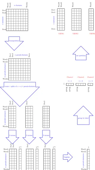
Doc1 Doc2 Docn Wo rd 1 Wo rd 2 Wo rd m mfeatures n instances transposition Word1 Word2 Wordm Do c1 Do c2 Do cn npseudo-features m pseudo-instances
creatersplits ofs=n/rpseudo-features
Word1 Word2 Wordm Do c9 Do c3 Do c5 Do c2 m pseudo-instances
k-means k-means k-means
λ(1) λ(2) λ(2) Word1 Word2 Wordm Do c9 Do c3 Do c5 Do c2 m pseudo-instances bagging Word1 Word2 Wordm ˆ λ m pseudo-instances group by label Wo rd 9 Wo rd 5 Wo rd 1 Wo rd 3 ˆ λ
Cluster1 Cluster2 Cluster3
λ= 1 λ= 2 λ= 3 use partition Doc1 Doc2 Docn Wo rd 9 Wo rd 5 Wo rd 1 Wo rd 3
VIEW1 VIEW2 VIEW3
n
instances
Fig. 1. Illustration of the overall process based on the reference example.
data-points (the pseudo-instances) we define the pairwise row distance as anL2distance, i.e. an Euclidean distancedE(·,·). The distance betweenrowyj androwyj is defined as
d(yj, yj) =d(j, j) = n i=1 (yj,i−yj,i)2 1 2
where i runs over all the pseudo-features (i.e. the former objects). Based on this distance one can run the clustering algorithm k-means [19] or another algorithm belonging to the same family, such as k-medoid [20].
2) Output of a single pseudo-instance clustering and di-mensionality problems: Running the k-means partitioning algorithm, one obtains a solution for the problem of pseudo-instance partitioning based on the dataset Y. This will also be a solution of the MVG (i.e. feature partitioning) problem based onX.
In practice, however when the number n of rows of X is large, after transposition, the number of pseudo-features (columns ofY) makes the clustering problem high-dimensional, and the clustering algorithm potentially less effective (e.g. a significant difference of two points along a dimension could be obfuscated by many non-significant differences along other dimensions).
One can address the issue by breaking the set of pseudo-features intorsmaller redundant subsets of selements each (approximately n/r elements each), then by running the clustering algorithm separately on the whole set of pseudo-instances, described only by a group of s pseudo-features. This yields r distinct cluster partitions. Eventually, the dif-ferent partitions can be aggregated by a partition consensus algorithm, to produce an individual partition solution.
In terms of our reference example – in which the objects are the documents and the features are the words, and in which the pseudo-instances are the words, while the pseudo-features are the documents – this corresponds to breaking the corpus into r randomly chosen groups of documents and running the clustering algorithmrtimes over all the pseudo-instances (words), using onlyspseudo-features at time, then aggregating the resultingrpartitions into a single solution partition: e.g. a word will be assigned to the partition block to which it belongs most often.
This task is formally described in the next subsection. C. The consensus clustering task
AclustererΦis a function that, given a setY, outputs a par-titionπunder the form of a label vectorλ. Differentclusterers
Φ(1),Φ(2), . . . ,Φ(r), run over the same datasetY will output, in general, different label vectorsλ(1), λ(2), . . . , λ(q), . . . , λ(r). A collection of label vectorsΛ ={λ(1), λ(2), . . . , λ(r)}can be combined into a single label vector λˆ, called consensus labelling, by using a consensus functionΓ. Equivalently one can say that Γcombines the corresponding collection Π of partitions Π = {π(1), π(2), . . . , π(q), . . . , π(r)} into a single partitionπˆ. Givenrpartitions, theλ(q)partition consisting in kclusters/blocks, a consensus function is defined as a mapping Nn×r → Nn taking a set of partitions into an integrated
partition,Γ : Λ→ˆλ, or equivalentlyΓ : Π→πˆ.
Theconsensus clustering problemconsists in finding a new partitionˆπof the dataY, given the partitions inΠ, such that the objects in a block/cluster ofπˆ are more similar (in some pre-specified sense) to each other, than the object in different clusters of πˆ. The solution of the problem can be defined in different ways [17]: some are based on minimization of information theoretic measures, some on different forms of aggregation, such as majority voting (bagging). We will use the latter approach. Beforehand, however we discuss a minor technical issue.
1) Logical equivalence: The reconciliation of the different partitions involves an ancillary issue: there are partitions that are denoted by different arrays of labels, but that are the same from the logical point of view (a suitable permutation of the symbols used to denote the labels is able to transform one
Fig. 2. Left: the first25images of the MNIST dataset. Right: the average gray-level taken over the whole set: the pictures hints at a ”background” region little or not used by the handwritten digits.
in another). Indeed, for each unique partition there are k! equivalent representations as integer label vectors: i.e. given two equivalent partitions there exists a permutation of the labels such that they become equal. Formally, given the set P of the k! permutations of [1, k], two label vectors λ(a) and λ(b) are said to be logically identical if there exist a permutation p ∈ P, taking λ(a) into λ(a) such that λ(a)(yj) =λ(b)(yj), ∀j∈[1, m]. One needs to account for
those equivalences, in order not to make the task of partition reconciliation uselessly complex: this issue can be solved passing to a canonical form [14]. Indeed the solution to this potentially complex correspondence problem is very simple. The pseudo-instances are endowed by a numerical index, setting a natural ordering for the set of pseudo-instances. After obtaining the rdifferent partitions from the rclusterers, one should rewrite, for each partition, the block labels, so that the index of the blocks is monotonic (e.g. monotonic non-decreasing) w.r.t. to the order of the objects. By rewriting each partition in this way, logically identical partitions will be mapped onto the same representation. Formally, one should enforce for each partition the constraints (i) λ(y1) = 1(the
first object defines the first block/cluster) and (ii) λ(yi+1)≤ maxj=1,...,i(λ(yj))+1∀i= 1,2, . . . ,(n−1)(the cluster label λ(yi+1)either has a label that occurred before, or has a label
that increases by one unit w.r.t. the highest used so far). 2) Partition reconciliation, by majority voting: Once the r partitions are in canonical form, it is straightforward to aggregate them into a single solution partitionλˆ: one assigns the pseudo-instance to its most frequently occurring label.
ˆ
λ(yj) = arg maxλ count(λ(yj))
In the reference example where the pseudo-instances are the words, this corresponds to assigning a word to the partition block in which it occurs most often. Ties can be resolved by random choice. The overall process is illustrated in Figure 1
IV. RESULTS
We demonstrate the proposed approach using the MNIST dataset containing gray-scale images of handwritten digits [18]. With respect to the document-word reference example, where we had documents we now have pictures, where we had word occurrence counts we have pixel gray levels.
A. The dataset
The dataset contains n= 60,000gray-scale images: each image instance represents a handwritten digit. Although the class label for each image is available (there are 10classes, {0,1,2, . . . ,9}), it is not used in our unsupervised setting. The features considered for each instance are the gray-scale intensities of the pixels, each intensity takes an integer value in the interval[0,255]. In the original version of the dataset each image has 28×28 = 784pixels (there are m= 784features for each instance). Thus, the dataset can be represented in terms of an= 60000 row andm= 784column table. B. The process
Our final goal was to obtain a partitioning of the columns intokviews, i.e. the whole area of the image inkpixel regions (later to be used separately to train distinct classifiers).
Following the above described approach, we transposed the table to obtain a table with m= 784rows (pseudo-instances, the pixels) and n = 60000 columns (pseudo-features, the images); then we broke this column set in r splits (each of s = n/r columns, i.e. images, chosen at random without restitution); using each split we rank-means using all them pseudo-instances, thus we obtainedrpartitions of the pseudo-instances; finally we reconciled the r partitions into a single partition solution, by majority voting.
Transposing back the partitioned data table we got a view partitioning of the image features, i.e. a partitioning of the pixels in regions that share some similarity. The similarity defined by the application of k-means was the co-occurrence of equal or similar gray-levels.
C. The outcomes
We experimented different values of the number-of-views parameterk(number of pixel regions,k={2,3,5,9,13,17}) and the split-granularity parameter r (and consequentlys =
n/r, number of images/features contained in a pseudo-feature split). We chose vales of r which together could represent almost the whole range, leaving out the extremities (the single ”split” case, withr= 1and the one-element split, withs= 1). The results are shown in Figure 3.
One can see, in the first row of Figure 3 (also with reference to Figure 2) that for k = 2 views, the process neatly distinguishes between the active region and the non-active region (whose pixels are almost never used). Fork= 3 views, one can distinguish further, inside the central active region, two sub-regions with different importance in detailing the digits. Withk= 5views, and up, the process issues views, which detail the difference of the regions even further; also the different values ofsreturn varying shapes.
V. VALIDATION
In principle, the views thus obtained could be later used for multi-view learning. This could consist either in unsupervised multi-view learning, e.g. multi-view clustering, or in super-vised ore semi-supersuper-vised multi-view learning. In the latter
k= 17 k= 13 k= 9 k= 5 k= 3 k= 2 r= 6 r= 12 r= 60 r= 120 r= 600 r= 3000 r= 6000 r= 12000 s= 10000 s= 5000 s= 1000 s= 500 s= 100 s= 20 s= 10 s= 5
Fig. 3. Outcome of the view splitting process for three different resolutions. Each color corresponds to a cluster of pixels and represents a view. The parameter kis the number of views. The number of instances used for the task wasn= 60000. The parametersris the number of independent k-means clustering processes obtained by sectioning the data, then reconciliated in a single clustering partition. Finally,s=n/r. See also text of the Results Section.
case the learning phase would involve the class labels: in our case study the symbol of the represented digit.
For instance in an hypothetical semi-supervised setting, one might know the class label only for a subset of images and might want to predict the class for the reminder images. This would be carried out by training distinct models separately on each view, and then using them to create the missing labels by means of co-training [4]. In this case, a direct validation of the effectiveness of our multi-view generation method could consist in a study of the quality of the co-training phase resulting from the use of the proposed MVG phase.
Such direct validation, however, would apply only to the specific multi-view technique considered. On the other hand, a wider systematic study of different multi-view techniques, would go beyond the scope of the present paper.
Nevertheless, it is possible to perform a indirect validation of the method, endowed by a reasonable generality, based on the following considerations. In a supervised multi-view setting, one requires that the views issued by the MVG phase fulfill some natural requirements [4]:
1) each view must individually, be endowed withpredicting power,
2) each view must holdunique informationabout the targets, 3) the different views should achieve prevalently consistent
predictions.
An indirect validation of our method can be performed by checking that the views generated fulfill those base require-ments. We opted for such an indirect validation. For the sake of simplicity, we did not consider the third requirement, which is more complex to account for with a high number of views and many classes. We focused on the first two requirements.
We ran two kinds of learning models on the views that were obtained by our method: a Na¨ıve Bayesian classifier (NB) and a Decision Tree (DT). Since the findings from the two learners were in qualitative agreement, hereafter, for space reasons, we report only about the NB classifier.
For each parameter setting (each sub-figure in Figure 3), we ran the learner(s) on all the views of the n = 60000 instances MNIST training set and measured the accuracy of the prediction using then= 10000instances MINT test set. We computed both the individual accuracy in the classification of each individual symbol/class (digits from0to9) and the average accuracy over all the classes. The results are shown in Figure 4 for some representative combination of parameters of thek= 3andk= 5views cases. For completeness we also computed the accuracy of the classifier defined by the bagged version of the different views. We also trained, for comparison, a single view NB classifier. The plots allow to appreciate both the predicting power of the individual views, and the fact that they are endowed with unique information about the targets.
1) Requirement 1: Predicting power.: The accuracy of the NB classifier trained on individual views, is always (up to the level studied of k = 17 views) much greater than the baseline random classifier (which would have accuracya = 0.10 for each target), and for small number of views (large amount of information in each view) is often comparable to the reference single view classifier accuracy,a= 0.84(this is the accuracy of the NB classifier applied to all the features/pixels, gathered into a single view). Looking at specific target classes one can observe that some views achieve a reasonably high performance at least on one class.
2) Requirement 2: Unique information on targets: As to this requirement, one could already qualitatively see, from Figure 3, that the views concretize in pixel areas covering regions, approximately corresponding to constructive elements of the digits: for instance for k = 9 (e.g. with r = 120), one can see distinctly that including or omitting some patches one can build the digit3or the digit9or the digit 8. Thus, each view holds information that is not available to others for determining the class of the image. This is confirmed in Figure 4. The views have different efficiencies for different targets: each view is the top accuracy view for at least one target. In other words, each view would have something to teach to the others, for example within a co-training process.
In short, both main requirements are fulfilled. VI. DISCUSSION,CONCLUSIONS AND OUTLOOK In this work we approached the Multi View Generation problem in an unsupervised, setting. We proposed an approach based on the transposition of the data table: the original instance rows are mapped into columns (the pseudo-features), while the original feature columns become rows (the pseudo-instances); the latter can then be partitioned by any suitable standard instance-partitioning algorithm: the resulting groups can be considered as groups of the original features, i.e. views, solution problem. We demonstrated the approach using k-means.
With reference to our document-word reference example, notice, for the sake of comparison, that the task of ”clustering words based on the documents to which they belong ” and the task of ”clustering documents based on the words that they contain” are commonly studied classical tasks. In the former task one assigns to the words the role of instances and the the documents the role of features; in the latter case it is the converse. However, in both classical cases, the final aim of the procedure is to come up with a clustering of the instances. Our approach, on the contrary, aims at producing a partition of the features into views (later to be used by independent prediction models).
Furthermore, the effectiveness of the two mentioned clas-sical tasks is quantified based on the quality of the instance partition or in relation to another reference partition: either based on intrinsic criteria (such as the goodness of clustering Hubert’s r statistics) or based on external criteria by com-paring the clusters to ground truth classes (e.g. using purity, Rand index, Jaccard index and so on). In our case, on the
contrary, the outcome of the partition is assessed in relation of the effectiveness of the multi-view partition in supporting a subsequent learning procedure.
Another technique worth mentioning, for comparison, is co-clustering [21], [22]. Co-clustering models the relation of words and documents as a bipartite graph: the co-clustering algorithms find sub-graphs of the initial connected component graph, using spectral methods. It is true that the output provides a clustering of the words and a clustering of the documents: the words (documents) belonging to the same subgraph are in the same word- (document-) cluster. It is also true that the method issues a simultaneous clustering of the features and of the instances. However, the method is radically different from ours, since it involves ajoint minimizationand in general will not provide the same results.
Our method provides an unsupervised multi view partition. As for any unsupervised optimization task, whose output is used in input of a supervised (or semi-supervised) task, issue might arise that the solution of the former task is not necessarily optimal to the latter. This is a problem that can be found in many settings, it can take place for instance, when using a learner after having applied Principal Component Analysis, or any other representation learner.
The point that we wanted to make is that one can take methods designed for working in instance space and use them in feature space. The application of such dual-space approach can be extended to many other situations, that will be the object of future works.
ACKNOWLEDGEMENTS
The authors acknowledge the support of the Informa-tion and CommunicaInforma-tion Technology Fund (ICT Fund) at EBTIC/Khalifa University, Abu Dhabi, UAE (Project number 88434000029). The work was partially founded also by the European Unions Horizon 2020 research and innovation pro-gramme, within the projects Toreador (grant agreement No. 688797), Evotion (grant agreement No. 727521) and Threat-Arrest (Project-ID No. 786890).
REFERENCES
[1] E. Damiani, G. Gianini, M. Ceci, and D. Malerba, “Toward iot-friendly learning models,” in 2018 IEEE 38th International Conference on Distributed Computing Systems (ICDCS), July 2018, pp. 1284–1289. [2] S. Sun, “A survey of multi-view machine learning,”Neural Computing
and Applications, vol. 23, no. 7-8, pp. 2031–2038, 2013.
[3] J. Zhao, X. Xie, X. Xu, and S. Sun, “Multi-view learning overview: Recent progress and new challenges,”Information Fusion, vol. 38, pp. 43–54, 2017.
[4] A. Blum and T. Mitchell, “Combining labeled and unlabeled data with co-training,” inProceedings of the eleventh annual conference on Computational learning theory. ACM, 1998, pp. 92–100.
[5] F. Feger and I. Koprinska, “Co-training using rbf nets and different feature splits,” inNeural Networks, 2006. IJCNN’06. International Joint Conference on. IEEE, 2006, pp. 1878–1885.
[6] S. Sun and F. Jin, “Robust co-training,”International Journal of Pattern Recognition and Artificial Intelligence, vol. 25, no. 07, pp. 1113–1126, 2011.
[7] S. Bickel and T. Scheffer, “Multi-view clustering.” in ICDM, vol. 4, 2004, pp. 19–26.
[8] A. Kumar, P. Rai, and H. Daume, “Co-regularized multi-view spectral clustering,” inAdvances in neural information processing systems, 2011, pp. 1413–1421.
all digits 0 1 2 3 4 5 6 7 8 9 0 0.1 0.2 0.3 0.4 0.5 0.6 0.7 0.8 0.9 1 1.1 1.2 0 . 6 0.6 0 . 8 0 . 6 0 . 52 0 . 39 0.42 0 . 86 0 . 77 0 . 3 0 . 66 0 . 7 0 . 81 0 . 89 0 . 61 0 . 78 0 . 64 0 . 44 0 . 8 0 . 72 0 . 64 0 . 6 0 . 75 0 . 92 0 . 9 0 . 59 0 . 75 0 . 69 0.69 0 . 8 0 . 77 0 . 71 0 . 69 0 . 8 0 . 91 0.93 0 . 73 0 . 84 0 . 73 0 . 62 0 . 89 0 . 83 0 . 72 0 . 77 accuracy k= 3,r= 3000,s= 20
’ view1 ’ ’ view2 ’ ’ view3 ’ ’ bagged views ’
all digits 0 1 2 3 4 5 6 7 8 9 0 0.1 0.2 0.3 0.4 0.5 0.6 0.7 0.8 0.9 1 1.1 1.2 0 . 55 0 . 48 0 . 88 0 . 57 0 . 42 0 . 25 0 . 38 0 . 87 0 . 73 0 . 17 0 . 68 0 . 62 0 . 72 0 . 94 0 . 48 0 . 68 0 . 49 0 . 37 0 . 74 0 . 71 0 . 42 0 . 59 0 . 63 0 . 72 0 . 81 0 . 6 0 . 58 0 . 58 0 . 23 0 . 81 0 . 73 0 . 51 0 . 65 0 . 64 0 . 79 0 . 92 0 . 63 0 . 48 0 . 57 0.59 0 . 7 0.71 0 . 48 0.51 0 . 54 0 . 82 0 . 73 0 . 34 0 . 75 0 . 38 0 . 24 0 . 68 0.69 0 . 5 0 . 26 0 . 8 0 . 96 0.97 0 . 75 0 . 81 0 . 72 0 . 55 0 . 91 0 . 87 0 . 65 0 . 78 accuracy k= 5,r= 120,s= 500
’ view1 ’ ’ view2 ’ ’ view3 ’ ’ view4 ’ ’ view5 ’ ’ bagged views ’
Fig. 4. Accuracies for Na¨ıve Bayes classifiers trained on individual views (colored bars) and performance of the bagged classifier (gray bars), for the different targets (digits 0 to 9, ten rightmost groups) and averaged over all the targets (first, i.e. leftmost group of bars). From the top to the bottom:k= 3views (with r= 3000ands= 20);k= 5views (withr= 120ands= 500).
[9] M. Legesse, G. Gianini, and D. Teferi, “Selecting feature-words in tag sense disambiguation based on their shapley value,” inSignal-Image Technology & Internet-Based Systems (SITIS), 2016 12th International Conference on. IEEE, 2016, pp. 236–240.
[10] M. Legesse, G. Gianini, D. Teferi, H. Mousselly-Sergieh, D. Coquil, and E. Egyed-Zsigmond, “Unsupervised cue-words discovery for tag-sense disambiguation: comparing dissimilarity metrics,” inProceedings of the 7th International Conference on Management of computational and collective intElligence in Digital EcoSystems. ACM, 2015, pp. 24–28.
[11] H. Mousselly-sergieh, E. Egyed-zsigmond, G. Gianini, M. Doller, H. Kosch, and J. Pinon, “Tag similarity in folksonomies,” inINFORSID. INFORSID, 2013, pp. 277–291.
[12] H. Mousselly-Sergieh, M. D¨oller, E. Egyed-Zsigmond, G. Gianini, H. Kosch, and J.-M. Pinon, “Tag relatedness using laplacian score fea-ture selection and adapted jensen-shannon divergence,” inInternational Conference on multimedia modeling. Springer, 2014, pp. 159–171. [13] H. Mousselly-Sergieh, E. Egyed-Zsigmond, G. Gianini, M. D¨oller,
J.-M. Pinon, and H. Kosch, “Tag relatedness in image folksonomies,”
Document num´erique, vol. 17, no. 2, pp. 33–54, 2014.
[14] A. Strehl and J. Ghosh, “Cluster ensembles—a knowledge reuse frame-work for combining multiple partitions,”Journal of machine learning research, vol. 3, no. Dec, pp. 583–617, 2002.
[15] S. Dudoit and J. Fridlyand, “Bagging to improve the accuracy of a clustering procedure,” Bioinformatics, vol. 19, no. 9, pp. 1090–1099,
2003.
[16] H. G. Ayad and M. S. Kamel, “Cumulative voting consensus method for partitions with variable number of clusters,”IEEE transactions on pattern analysis and machine intelligence, vol. 30, no. 1, pp. 160–173, 2008.
[17] J. Ghosh and A. Acharya, “Cluster ensembles,”Wiley Interdisciplinary Reviews: Data Mining and Knowledge Discovery, vol. 1, no. 4, pp. 305– 315, 2011.
[18] Y. LeCun, C. Cortes, and C. Burges, “Mnist handwritten digit database,”
AT&T Labs [Online]. Available: http://yann. lecun. com/exdb/mnist, vol. 2, 2010.
[19] J. MacQueenet al., “Some methods for classification and analysis of multivariate observations,” inProceedings of the fifth Berkeley sympo-sium on mathematical statistics and probability, vol. 1, no. 14. Oakland, CA, USA., 1967, pp. 281–297.
[20] X. Li,K-Means and K-Medoids. Boston, MA: Springer US, 2009, pp. 1588–1589.
[21] I. S. Dhillon, “Co-clustering documents and words using bipartite spec-tral graph partitioning,” inProceedings of the seventh ACM SIGKDD international conference on Knowledge discovery and data mining. ACM, 2001, pp. 269–274.
[22] I. S. Dhillon, S. Mallela, and D. S. Modha, “Information-theoretic co-clustering,” inProceedings of the ninth ACM SIGKDD international conference on Knowledge discovery and data mining. ACM, 2003, pp. 89–98.