Strategic Planning
M.-T. Nguyen & M. Dunn
Joint Operations Division
Defence Science and Technology Organisation
DSTO–TR–2242
ABSTRACT
Scenarios are an important tool in the strategic planning process, and are increasingly used in both the Defence and business world. This paper describes some potentially useful scenario analysis methods for systematically selecting and developing future scenarios. The processes of each method are illustrated with small examples. We also demonstrate a single, flexible approach to combining these methods using a typical Defence strategic planning problem. Some general guidelines to consider when choosing and using an appropriate scenario analysis method are also discussed.
Published by
Joint Operations Division
DSTO Defence Science and Technology Organisation Fairbairn Business Park,
Department of Defence, Canberra, ACT 2600. Telephone: (02) 6265 9111 Facsimile: (03) 6265 2741 c Commonwealth of Australia 2009 AR No. AR–014–379 February 2009
Some Methods for Scenario Analysis in Defence Strategic
Planning
Executive Summary
Scenarios are an important tool in the strategic planning process, and are increasingly used in both the Defence and business world. Scenario analysis has emerged as a tool for strategic planning when the future is perceived as surrounded by a high degree of uncertainty and complexity. Scenario analysis techniques characteristically synthesise quantitative and qualitative information, constructing multiple scenarios or alternative portraits of the future.
Scenario analysis consists of the three basic stages: (1)Problem analysisto come up with an exact definition for the problem of the investigation; (2) System analysis to identify relevant external influences on the problem to be investigated, and (3)Synthesis processto examine the existing interdependencies between the influencing factors and to establish alternative scenarios.
Problem analysis helps all experts and stakeholders gain a common understanding of the problem at hand. Based on this consensus the problem can be further bounded and structured. System analysisexpresses the problem as a system of inter-related dynamic components (subsystems), with the system itself linked to its external environment. From every subsystem, a number of representative influencing factors relevant to the problem are then identified.Synthesis processestablishes a logical and systematic way for scanning the range of possible scenarios and for selecting main scenarios or choosing a set of scenarios that includes all plausible futures.
A variety of creative methods such as brainstorming, brainwriting, round table dis-cussion, and the Delphi technique can be employed in the first two analysis stages. There are two basic methodologies for implementing the second and especially the third stage of the scenario analysis: (1) Non-Bayesian method (e.g. Morphological Analysis, Battelle approach, Field Anomaly Relaxation) and (2)Bayesianmethod (e.g. Cross-Impact Analysis). Some extensions based on both classes are also developed (e.g. Battelle approach with Cluster Analysis, Cross-Impact Analysis with Integer Programming). This report describes these scenario analysis methods and provides a possible way for combining them into a single more flexible approach. The processes and mathematical formulation of each method is presented in this paper, as well as with a discussion of the pros and cons of employing these methods. The combined approach is illustrated with a typical example and numerical experiment. This approach enables the scenario development process to start with relatively simple information, gained from experts and problem-owners, and through a rigorous and transparent process identifies a manageable set of representative or balanced scenarios.
To carry out the combined approach, information about the mathematical formulation of each method has been used to generate algorithms for developing computer decision support tools. These decision support tools automate complex calculations and enable users to use and combine the techniques without in depth knowledge of the mathematical aspects. The paper concludes by emphasising some general points to consider when choosing and using an appropriate scenario analysis method in Defence strategic planning.
Authors
Minh-Tuan Nguyen Joint Operations Division
Minh-Tuan received his DipSc from Paul Sabatier University at Toulouse, France in 1991, BSc(Hons) in 1996 and PhD in 2000, both from the University of South Australia. He has experience in the fields of operations research, mathematical modelling & simulation, control systems and differential games. Since joining DSTO in late 2000, he has worked on force mix options, provided scientific & technical advice on methods and processes dealing with Defence strategy, capability plan-ning and decision making as well as explored concepts and developed suitable techniques & decision support tools for analysing and assessing future scenarios.
Madeleine Dunn Joint Operations Division
Madeleine has a Bachelor of Science (Cognitive Science) from Flinders University of South Australia and is currently study-ing a Master of Science (Cognitive Science) through Adelaide University. She began work with the Defence Signals Direc-torate in 2002 and joined DSTO in 2005. Since joining DSTO, Madeleine has worked on Defence experimentation programs as well as conducting research in qualitative operations re-search methods and techniques in strategic analysis. She currently works as an operations analyst within Joint Oper-ations Division. Madeleine is employed within DSTO Sup-port to Operations, where she provides reachback supSup-port to deployed analysts. Madeleine is also an Army Reservist with the Australian Army Psychology Corps.
Contents
1 Introduction 1
2 Scenario Analysis Methodology: An Overview 1
3 Non-Bayesian Method 2
3.1 Morphological Analysis (MA) . . . 2
3.1.1 Description . . . 2
3.1.2 Application Issues . . . 3
3.2 Field Anomaly Relaxation (FAR) Analysis . . . 4
3.2.1 Description . . . 4
3.2.2 Application Issues . . . 6
3.3 Battelle Approach . . . 7
3.3.1 Description . . . 7
3.3.2 Application Issues . . . 8
4 Bayesian Method - Cross-impact analysis 9 4.1 Model Settings . . . 9
4.2 Sarin’s Model - System of Equations . . . 10
4.3 De Kluyver’s & Moskowitz’s Model - Goal Programming . . . 11
4.4 Application Issues . . . 14
5 Extended Methods 14 5.1 Modified Goal Programming . . . 14
5.1.1 Formulation . . . 14
5.1.2 Application Issues . . . 16
5.2 Cluster Analysis - Representative Scenarios . . . 16
5.2.1 Measures of Similarity . . . 16
5.2.2 Cluster Methods . . . 17
5.2.3 Application Issues . . . 17
5.3 Integer Linear Programming - Balanced Mix of Scenarios . . . 18
5.3.1 Formulation . . . 18
6 An Approach of Combining Methods 20
6.1 Typical Example . . . 20
6.2 Six-step Approach of Combining Methods . . . 20
6.2.1 Description of Future States . . . 21
6.2.2 Assessment of States’ Compatibilities . . . 22
6.2.3 Determination of Compatible Scenarios . . . 23
6.2.4 Assessment of States’ Possibilities . . . 24
6.2.5 Analysis of Scenarios’ Possibilities . . . 24
6.2.6 Determination of Main Scenarios . . . 25
7 Conclusion 28 References 29
Appendices
A Modelling Goal Programming with AMPL 32 A.1 Model File “GP.mod” for GP Formulation . . . 32A.2 Command Script File “GP.run” for Running Model . . . 33
B Modelling Modified GP and ILP with AMPL 34 B.1 Model File “mGP-MIP.mod” . . . 34
B.2 Command Script File “mGP-MIP.run” . . . 35
Figures
1 Scenario-building through Morphological Analysis . . . 32 A Typical Scenario Tree . . . 6
Tables
1 Matrix of Pairs . . . 52 Filtering Inconsistent/Implausible Configurations . . . 5
3 Terms Used in the non-Bayesian Methods . . . 7
4 Factors, Outcomes and Compatibility Ratings . . . 8
5 Scenarios with Worst/Average Compatibility Values . . . 8
6 List of Scenarios . . . 9
7 Marginal Probabilities . . . 11
8 Joint Probabilities . . . 11
9 Conditional Probabilities . . . 12
10 Scenarios Probabilities . . . 13
11 Conditional Probabilities & Deviations . . . 13
12 Six-step Approach of Combining Methods . . . 21
13 Australia’s Regional Environment in 2030: A Morphological Analysis . . . . 21
14 Sample Data . . . 22
15 Selected Compatible Scenarios . . . 24
16 Scenarios Probabilities . . . 25
17 Sample of Cluster Analysis . . . 25
1
Introduction
Scenario analysis has emerged as a tool for strategic planning [7] when the future is perceived as surrounded by a high degree of uncertainty and complexity. Scenario anal-ysis techniques characteristically synthesise quantitative and qualitative information, constructing multiple scenarios or alternative portraits of the future.
Scenarios are an important tool in the strategic planning process, and are increasingly used in both the Defence and business world. This report describes some scenario analysis methods and provides a possible way for combining them into a single more flexible approach. The combined approach is illustrated with a typical example and numerical experiment. This approach enables the scenario development process to start with relatively simple information (from experts and problem-owners) and through a rigorous and transparent process identifies a manageable set of representative or balanced scenarios.
After providing an overview of scenario analysis methodology in section 2, the next three sections of the report review specific methods. The processes and mathematical formulation of each method is presented, as well as with a discussion of the pros and cons of each method. This information has been used to generate algorithms for developing computer decision support tools (Section 6, see also [5]). It should be noted that the list of methods is notexhaustive, and other techniques are available in the list of related publications [7, 16, 32]. What is presented here, however, is a cross-section of techniques that provide rigorous and transparent methods of generating scenarios for complex strategic planning problems. In Section 6, we present a six-step approach to combining methods, which is demonstrated by an illustrative example. The report finally concludes by emphasising some general points to consider when choosing an appropriate scenario analysis technique in Defence strategic planning.
2
Scenario Analysis Methodology: An Overview
In this report, we consider a scenario analysis consisting of the three basic stages (cf. [1]): 1. Problem analysis: to come up with an exact definition for the problem of the
investigation.
2. System analysis:to identify relevant external influences on the problem investigated. 3. Synthesis process: to examine the existing interdependencies between the
influenc-ing factors and to establish alternative scenarios.
The problem analysis stage helps all experts and problem-owners gain a common understanding of the problem at hand. Based on this consensus the problem can be further bounded and structured. The system analysis expresses the problem as a system of inter-related dynamic components (subsystems), with the system itself linked to its external environment. From every subsystem, a number of representative influencing
factors relevant to the problem are then identified. The synthesis process establishes a logical and systematic way for scanning the range of possible scenarios and for selecting main scenarios or a balanced mix of scenarios.
A variety of creative methods such as brainstorming, brainwriting, round table discus-sion, and the Delphi technique [14] can be employed in the first two analysis stages. There are two basic methodologies for implementing the second and especially the third stage of the scenario analysis:
• Non-Bayesianmethod (e.g. Morphological Analysis (MA) [35], Battelle approach [32], Field Anomaly Relaxation (FAR) [2, 3, 20, 21])
• Bayesianmethod1(e.g. Cross-Impact Analysis using a system of equations [24, 25], or Goal Programming (GP) [4]).
Some extensions based on both classes are also developed (Battelle approach with Cluster Analysis [1], GP with Integer Programming [12], or Fuzzy Logic [26, 27, 33]). These are described in detail in the following three sections.
3
Non-Bayesian Method
3.1
Morphological Analysis (MA)
3.1.1 Description
Morphological analysis was first developed by Fritz Zwicky, the Swiss astrophysicist and aerospace scientist based at the California Institute of Technology, during the Second World War [35]. Essentially, morphological analysis is a method for identifying and investigating the total set of possible relationships contained in a multidimensional problem [23].
Firstly, the system or function under examination is broken down into subsystems (components or dimensions). In this breakdown of the system, the choice of components is critical and requires considerable thought which can be based on results of the problem analysis (e.g. from brainstorming). The aggregation of components must also represent the whole system. Too many components avoids a clear analysis; conversely, too few makes for an oversimplified analysis. Obviously a workable compromise must be found. It should be noted that too many and too few are subjective based on the needs of the analysis.
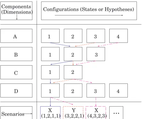
Each component can take on several configurations (states or hypotheses). A given scenario is characterised by the choice of a specific configuration for each of the components. There are as many possible scenarios as there are combinations of configurations. All these combinations represent the field of possibilities, called the morphological space.
1The central idea of the Bayesian method is to elicit the likelihood distribution for future scenarios to be projected from the experts in the field.
Components (Dimensions) A B C D Scenarios
Configurations (States or Hypotheses)
1 2 3 4 1 2 3 1 2 1 2 3 4
...
X (1,2,1,1) Y (3,2,2,1) X (4,3,2,3)Figure 1: Scenario-building through Morphological Analysis
For instance, a generic example of scenario building through morphological analysis is shown in Figure 1. The morphological space presented is composed of 4 components; each having between two to four configurations. This enables one to identify a number of possible combinations (i.e. 96), that is the product of the number of configurations (4×3×2×4).
However, certain combinations and even certain families of combinations are unfeasible (e.g. incompatibility between configurations). The next phase, therefore, consists of reducing the initial morphological space to a useful subspace, by introducing exclusion factors or selection of criteria (e.g. economic, technical), from which the relevant combinations can be examined (for more details see Section 3.2 or Section 3.3).
3.1.2 Application Issues
Although the method has been used in technological forecasting [16, 19], it lends itself well to the construction of scenarios, in which the Social, Technology, Economics, Ecology, Politics, and Values2(STEEPV model - the six themes for thinking about the future [15])
dimensions can be characterised by a certain number of possible states. A scenario thus becomes nothing more than a route, a combination bringing together a configuration for each component. Morphological analysis therefore stimulates the imagination and enables one to scan the field of possibilities systematically.
The first limitation of MA stems from the choice of components. By leaving out a component or simply a configuration that is essential for the future, one runs the risk of leaving out one complete facet from the range of possibilities.
The second limitation, of course, stems from the sheer bulk of combinations which can rapidly submerge the user. Therefore, MA without computer support severely limits the number and range of parameters that can be employed.
In the next two sections, we will investigate two forms of MA. The first one [21] was developed by Rhyne and later [2, 3] used by Coyle, Crawshay, McGlone and Sutton where the phrase “field anomaly relaxation” is applied to a systematic approach for reducing the morphological space. Another form of MA mostly appears in German literature, developed by Battelle Institute in Frankfurt [32].
3.2
Field Anomaly Relaxation (FAR) Analysis
3.2.1 Description
Field Anomaly Relaxation (FAR) [20] uses the same structure as MA but changes its terminology. A problem space in FAR is divided into various fields (called ‘Sectors’), and within these fields, there are different descriptions of possible states (called ‘Factors’) that this field can take. A configuration is formed when one factor from each sector is combined, forming a Whole Field descriptor of an overall condition within the problem space. A part of the process for FAR is giving it asymbolic name(e.g. the OPTEC model: the letters (symbols) comprising the name OPTEC in [30] were chosen from sector names: pOlitical, Physical, Technical, Economic and Cultural environments) and then using these symbols to describe the configurations (e.g.O1P2T2E2C2means the first sector takes
thefirstfactor value and all other sectors take the correspondingsecondfactor value). Some configurations (combinations of the factors of the different sectors) can be elimi-nated as being not plausible to occur in real life (relaxation of anomalies) which reduces the span of possibilities of future developments. This process is calledfilteringin FAR. The first filter is to create amatrix of pairs. Using a simple scoring yes/no, experts answer the same question for each: ‘Can we think of a pattern within which these two factors might coexist?’
When a matrix is fully scored, all configurations containing inconsistent pairs (having pair(s) scored ‘no’) can be removed from consideration.
The second filter is to judge the wholeness of entire configurations. The coherence of each whole pattern is considered as certain combinations of pairs may be reasonable, but when put together, produce a scenario which is not sensible.
Wall posting of the remaining configurations seems almost necessary with repeated consideration of questions such as “How much more plausible is this configuration than that one?”
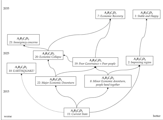
The last process in FAR is to compose scenarios. The surviving whole field configurations are positioned on a tree, in which nodes represent possible future states and branches represent transitions from one configuration to the next. Narratives are developed around these transitions and states, which then are formed into scenarios.
A scenario/future/‘Faustian’ tree is developed indicating possible pathways from con-figuration to concon-figuration and endpoints, ranging from positive transitions to the right side of the graph, and negative transitions, on the left hand side of the graph. While the vertical dimension represents time starting from present and spanning up to considered future times. It should be noted that neither dimensions represents a linear scale.
If a snapshot of a possible future is required, then a single configuration may be expanded out into a scenario. If a potential transition from the current state to a future state is important (possibly to investigate shaping strategies), then a chain of configurations may be used to develop the scenario.
Note that the tree presentation is intuitive in nature and a matter of imaginary (we don’t really know what we have until we try!). Early designation of scenario themes may ease scenario composition and help to match configurations with postulated scenario lines.
Table 1: Matrix of Pairs
A1 A2 B1 B2 C1 C2 D1 D2 D3 A1 A2 B1 X B2 C1 C2 X D1 D2 D3 X X
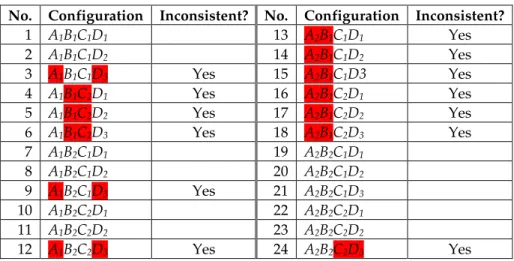
Table 2:Filtering Inconsistent/Implausible Configurations
No. Configuration Inconsistent? No. Configuration Inconsistent? 1 A1B1C1D1 13 A2B1C1D1 Yes 2 A1B1C1D2 14 A2B1C1D2 Yes 3 A1B1C1D3 Yes 15 A2B1C1D3 Yes 4 A1B1C2D1 Yes 16 A2B1C2D1 Yes 5 A1B1C2D2 Yes 17 A2B1C2D2 Yes 6 A1B1C2D3 Yes 18 A2B1C2D3 Yes 7 A1B2C1D1 19 A2B2C1D1 8 A1B2C1D2 20 A2B2C1D2 9 A1B2C1D3 Yes 21 A2B2C1D3 10 A1B2C2D1 22 A2B2C2D1 11 A1B2C2D2 23 A2B2C2D2 12 A1B2C2D3 Yes 24 A2B2C2D3 Yes
A1B2C2D2
11: Current State
A2B2C2D1
22: Major Economic Downturn
A1B2C1D2
8: Minor Economic downturn, people band together
A2B2C1D2
20: Economic Collapse
A2B2C1D1
19: Poor Governance = Poor people
A1B2C1D1 7: Economic Recovery A1B2C2D1 10: EARTHQUAKE! A2B2C1D3 21: Insurgency concerns A1B1C1D2 2: Improving region A1B1C1D1
1: Stable and Happy
2015 2025 2035
worse better
Figure 2:A Typical Scenario Tree
(4 sectors). Each sector consists of 2 factors except the last one (D) having 3 factors. There is thus 23×3=24 possible configurations. Suppose the matrix of pairs is given in Table 1 with inconsistent pairs marked with a ‘X’. Table 2 lists all configurations. Those without inconsistent pairs (11 configurations in this example) can be investigated as a whole, to judge the coherence of the complete configuration.
Assume that only 10 configurations survive after the second filtering. To construct a scenario tree, one may first choose a configuration for the current state, then affix each remaining configuration with a scenario theme and place them on the graph based on its timeframe. A typical scenario tree may be arranged as shown in Figure 2 (for illustrative purpose only).
3.2.2 Application Issues
As FAR is a form of MA, all pros and cons of MA will be seen in FAR. It offers a systematic and disciplined approach to the formulation and manipulation of data and ideas, also a way of reducing the number of scenarios in MA to a manageable set. However, there is a considerable amount of time and effort required from participants. Several workshops for a particular FAR analysis is a common practice [28, 30]. Indeed, FAR inventor, Russell Rhyne, proposes that participants should spend at least a week just looking and thinking about the scenario tree [21, 22].
The filtering process is a tedious, error-prone task when done by hand. A computer support tool should be used to automate some of FARs processes. Although, analysing and interpreting data and results must be cautiously scrutinised by experts.
Some FAR analysis [2] uses a very conservative approach and eliminates combination pairs only if there is consensus within the groups of experts. After eliminating all scenarios that contain factor value pairs that are declared impossible, the process is usually terminated (i.e. only first pass filtering).
Lack of certainty about the implausibility of particular factor value pairs will cause such pairs, and futures containing them, to be retained. Furthermore, the consistency of each whole pattern (carried out in second pass filtering) may be difficult for experts to determine with confidence. However, it may be possible to eliminate them when probability estimates are applied. This will be explained and illustrated in the Bayesian methods.
3.3
Battelle Approach
3.3.1 Description
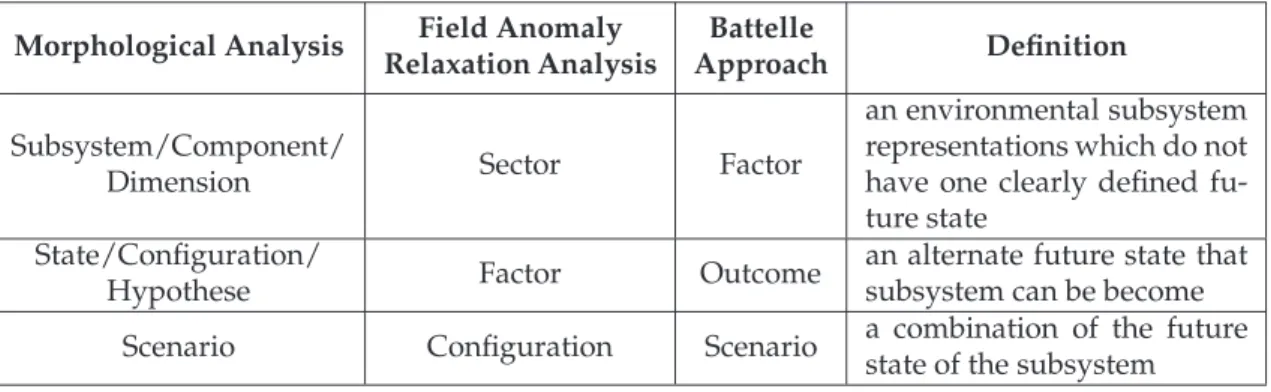
The ‘Battelle’ approach from Battelle Institute in Frankfurt [32] defines future states of the environmental subsystems by factoroutcomes. Here, the outcomes are specified mutually exclusively but exhaustively for certainfactors. Its structure is the same as Morphological Analysis (MA), but uses different terms. A comparison of main terms used in the non-Bayesian methods is listed in Table 3.
Table 3:Terms Used in the non-Bayesian Methods
Morphological Analysis Field Anomaly
Relaxation Analysis
Battelle
Approach Definition
Subsystem/Component/
Dimension Sector Factor
an environmental subsystem representations which do not have one clearly defined fu-ture state
State/Configuration/
Hypothese Factor Outcome
an alternate future state that subsystem can be become
Scenario Configuration Scenario a combination of the future
state of the subsystem
As a non-Bayesian method, the Battelle approach explicitly does not use probabilities; instead, it determines the interdependence between the individual outcomes by asking experts to rate the compatibility/plausibility of each outcome pair. The subjective estimates are called compatibility ratings, which are expressed on a scale from 1 to 5. A compatibility rating of 5 indicates two possible occurrences are very compatible, and a rating of 1 indicates they are not likely to occur together. Values of 2, 3, and 4 represent increasing compatibility.
The output is a range of compatible scenarios and their average compatibility values. One may choose certain scenarios for further analysis based on average compatibility value or worst compatibility value criteria.
For instance, assume the scenario in a future environment is mainly determined by three critical factorsx1,x2 andx3, and each factor consist of two mutually exclusive but
exhaustive outcomesxk,1andxk,2, k=1, 2, 3.
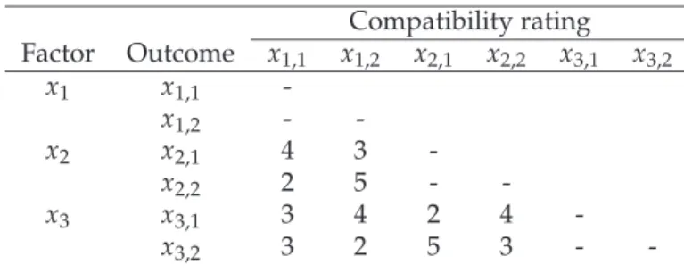
Table 4:Factors, Outcomes and Compatibility Ratings
Compatibility rating Factor Outcome x1,1 x1,2 x2,1 x2,2 x3,1 x3,2 x1 x1,1 -x1,2 - -x2 x2,1 4 3 -x2,2 2 5 - -x3 x3,1 3 4 2 4 -x3,2 3 2 5 3 -
-Assume further that the subjective estimates (Table 4) give us a compatibility rating (kij),∀i,j=1, . . . , 6 which is represented as a triangular matrix (kij =kji). In this example,
there are 23 = 8 possible scenarios (outcome combinations). Their worst and average
value compatibility is shown in Table 5.
Table 5: Scenarios with Worst/Average Compatibility Values
Compatibility
Scenario Set Worst value Average value
(1)x1,1x2,1x3,1 (4, 3, 2) 2 3.00 (2)x1,1x2,2x3,1 (2, 3, 4) 2 3.00 (3)x1,1x2,1x3,2 (4, 3, 5) 3 4.00 (4)x1,1x2,2x3,2 (2, 3, 3) 2 2.67 (5)x1,2x2,1x3,1 (3, 4, 2) 2 3.00 (6)x1,2x2,2x3,2 (5, 2, 3) 3 3.33 (7)x1,2x2,1x3,2 (3, 2, 5) 2 2.67 (8)x1,2x2,2x3,1 (5, 4, 4) 4 4.33
When we use the worst compatibility value criteria, the top three scenarios 3, 6 and 8 are recommended for further analysis while only scenario 4 and 7 are eliminated from the selection process if using the average compatibility value≥3 criteria.
3.3.2 Application Issues
Like FAR, the Battelle approach uses MA structure to break down problems into factor outcomes, which are specified mutually exclusive and exhaustive. Therefore, the imcompatible/inconsistent outcome combinations (scenarios) are deleted, and those scenarios with high compatibilities remain.
The Battelle approach uses a 5 point scale to obtain the compatibility estimates for every possible pair of factor outcomes. It provides a more flexible scheme for experts to rationalise their assessments, but may also take longer to determine their ratings.
As a non-Bayesian method, the Battelle approach does not consider the probabilities of outcomes, therefore, the selected scenarios may not correspond to real states (scenarios may have very small probabilities and could not practically be a basis of a meaningful planning effort). We will consider a modified approach by combining all techniques later.
4
Bayesian Method - Cross-impact analysis
Much of the writing about the future continues to be in the area of speculation [9], either in the sense of constructing scenarios reflecting the writer’s expectations of likely developments or in the sense of advocating changes in current conditions that are thought to be desirable. But in the long run the message of such speculative endeavours remains unconvincing unless there is a parallel development of analytical methods by which to derive reliable forecasts and consequent estimates of the relative likelihood of scenarios of the future, as well as measures for attaining desirable futures and plans for implementing such measures. Knowledge of the likelihoods of future scenarios is needed for planning in industry and government [24]. Thus the central idea of the Bayesian method is to elicit the likelihood distribution for the variable to be projected from the experts in the field.
4.1
Model Settings
Cross-impact analysis techniques [8, 9, 24, 25] make assumptions about the future developments in the environment of an organisation, in which certain factors influencing the problem under investigation are identified and either occur or do not occur3. Starting with a finite set of factors xi (i = 1, . . . ,n), scenarios consisting of combinations of
occurring and non-occurring factors are constructed in the synthesis phases.
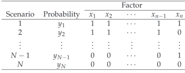
Table 6:List of Scenarios
Factor Scenario Probability x1 x2 · · · xn−1 xn 1 y1 1 1 · · · 1 1 2 y2 1 1 · · · 1 0 .. . ... ... ... ... ... ... N−1 yN−1 0 0 · · · 0 1 N yN 0 0 · · · 0 0
3It should be noticed that the Bayesian method does not require an MA structure (i.e. to break down problems into future states, which are specified mutually exclusive and exhaustive). Modified models will be presented in Section 5.1 to make the Bayesian method applicable to any problem with an MA structure.
The combination of n given factors x1, . . . ,xn produces N = 2n scenarios. Table 6 is a
scenario list where the likelihood or probability of a scenario, an unknown, is denoted by the variable ys,s = 1, . . . ,N; the number 1 shows that the factor occurs and 0 indicates
that it does not occur.
Two most recent techniques [4, 24, 25] employing cross-impact analysis have modelled the interdependencies between different factors in the form of conditional probabilities p(i|j) (the probability that factor xi will occur given that factor xj has occurred).
By solving systems of linear equations or linear programming models, the scenario likelihoods or its bounds are determined from the marginal and conditional probabilities. We now examine the mathematical formulation of these two models with a small numerical example.
4.2
Sarin’s Model - System of Equations
In Table 6, leta1, . . . ,anbe the column vectors of 0’s and 1’s ,ythe column vector of the
scenario probabilitiesysandytthe corresponding transposed vector ofy. The probability
vectorymust satisfy the following system of linear equations [24, 25]: ytai = p(i), i=1, . . . ,n yt(ai∧aj) = p(ij), i=1, . . . ,n; j>i yt(ai∧aj∧ak) = p(ijk), i=1, . . . ,n; j>i; k> j (1) .. . ... ... yt(a1∧a2∧. . .∧an) = p(12 . . .n), N
∑
s=1 ys =1, ys≥0, ∀swhere the ‘∧’ operation indicates a component by component multiplication of two vectors.
A sequential approach to determining scenario probabilities ys has been developed as
follows:
• Experts firstly provide marginal probabilitiesp(i).
Then the bounds on the joint probabilities p(ij) (where p(ij)def=p(i|j)p(j), the probability that factors xi andxj both occur) or conditional probabilities p(i|j)can
be calculated using standard probability theory.
• Experts can then supply additional estimatesp(i|j)within these particular bounds. In a sequential manner the bound on higher ordered joint probabilities are com-puted and in turn used by the experts.
Once the right-hand side of the system (1) is specified (by the sequential procedure), the solution of the system provides the scenario probability vector y. This allows us to
Table 7:Marginal Probabilities p(i) Value p(1) 0.7 p(2) 0.8 p(3) 0.3 p(4) 0.5
Table 8:Joint Probabilities
p(ij) Lower bound Upper bound p(12) 0.5 0.7 p(13) 0.0 0.3 p(14) 0.2 0.5 p(23) 0.1 0.3 p(24) 0.3 0.5 p(34) 0.0 0.3
rank the scenario in order of their likelihoods and select probable/possible scenarios for further analysis.
For example, in a four-factor scenario analysis, the marginal probabilities of occurrence for each factor has been assessed in Table 7. Using the following conditions on the joint probabilities p(ij),
max{0,p(i) +p(j)−1} ≤p(ij)≤min{p(i),p(j)}, i=1, 2, 3, 4 andj>i, the bounds onp(ij)are calculated and given in Table 8.
Within these bounds, Experts can now specify the joint probabilities (e.g. p(12) = 0.65, p(13) =0.25,p(14) =0.25,p(23) =0.25,p(24) =0.35 andp(34) =0.1).
Note that we don’t illustrate in the example above the iterations for estimating second-and higher-order joint probabilities as the next model using Goal Programming (GP) formulation will remove the need of such estimates which are not very appealing to participants.
4.3
De Kluyver’s & Moskowitz’s Model - Goal Programming
This model only requires the marginal probabilities p(i)and the first-order conditional probabilities p(i|j) with its bounds p(i|j)− and p(i|j)+ (the minimum and maximum of p(i|j), respectively). Recognising possible inconsistency between the estimates of the conditional probabilities and the marginal probabilities, the model using Goal Programming (GP) formulation seeks to find consistent values from which, in turn, the probability of each scenario can be computed.
It introduces the theoretically accurate conditional probabilities p∗(i|j)which fulfill the axioms of probability theory. In the formulation, the inconsistency is written in the form
p∗(i|j) +δ−
ij −δij+= p(i|j),
where the deviation termsδ−
ij andδ
+
ij measure the inconsistency (the difference between
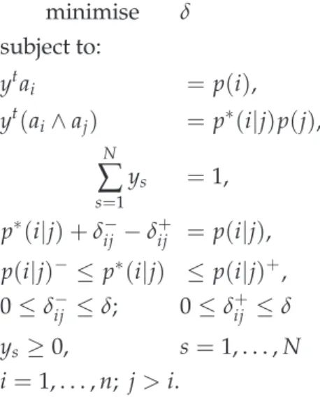
The objective of this GP is to minimise the maximum deviation which is denoted by δdef= max{δ−
ij,δ
+
ij}. The GP is of the form [4]:
minimise δ subject to: ytai = p(i), yt(ai∧aj) = p∗(i|j)p(j), N
∑
s=1 ys =1, (2) p∗(i|j) +δ− ij −δ+ij = p(i|j), p(i|j)−≤ p∗(i|j) ≤ p(i|j)+, 0≤δ− ij ≤δ; 0≤δ + ij ≤δ ys ≥0, s=1, . . . ,N i=1, . . . ,n; j>i.Any solution to GP in (2) will yield a set of the scenario probabilities ys, corrected
conditional probabilities p∗(i|j)and their deviationsδ−
ij,δ
+
ij from the most likely assessed
valuesp(i|j). Upon observing the results, the experts may wish to revise the assessment. This method is illustrated next using a small numerical example.
Suppose that the four-factor scenario analysis presented in Section 4.2 is considered. The marginal probability judgements are elicited in Table 7. To formulate the GP, we also need to estimate the most likely value of the conditional probabilities p(i|j)together with its boundsp(i|j)−andp(i|j)+.
The probability estimatesp(i), p(j)andp(i|j)to be consistent, must satisfy the following conditions max 0, p(i) +p(j)−1 p(j) ≤ p(i|j)≤min 1, p(i) p(j) , i=1, 2, 3, 4 andj>i.
From the above condition, one can thus obtain the bounds p(i|j)− and p(i|j)+. We suppose further that p(i|j)is specified within these bounds and given in the last column of Table 9.
Table 9:Conditional Probabilities
Pairwise factor Lower bound Upper bound Likely value
(i,j) p(i|j)− p(i|j)+ p(i|j)
(1,2) 5/8 7/8 0.7 (1,3) 0 1 0.5 (1,4) 2/5 1 0.8 (2,3) 1/3 1 0.7 (2,4) 3/5 1 0.8 (3,4) 0 3/5 0.5
Using any mathematical modelling language (e.g. AMPL [6]), we can formulate the GP in (2) as an input model (see Appendix A for an AMPL implementation) and the values in Table 7 and Table 9 as input data. The scenario probabilitiesysfor the example is shown
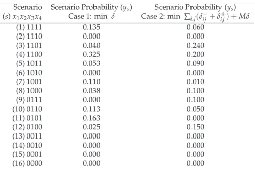
in Table 10. The deviation from any of the assessments is also obtained in Table 11. The Minmax objective (minδ) is used in the first case which results the change in all most likely values of the conditional probabilities (third column in Table 11) and the likely scenarios requiring further analysis are determined as 1, 4, 7, 10 and 11.
Table 10:Scenarios Probabilities
Scenario Scenario Probability (ys) Scenario Probability (ys)
(s)x1x2x3x4 Case 1: min δ Case 2: min ∑i,j(δij−+δ+ij) +Mδ
(1) 1111 0.135 0.060 (2) 1110 0.000 0.000 (3) 1101 0.040 0.240 (4) 1100 0.325 0.200 (5) 1011 0.053 0.090 (6) 1010 0.000 0.000 (7) 1001 0.110 0.010 (8) 1000 0.038 0.100 (9) 0111 0.000 0.100 (10) 0110 0.113 0.050 (11) 0101 0.163 0.000 (12) 0100 0.025 0.150 (13) 0011 0.000 0.000 (14) 0010 0.000 0.000 (15) 0001 0.000 0.000 (16) 0000 0.000 0.000
Table 11:Conditional Probabilities & Deviations
Pairwise factor Assessment Case 1 Case 2 Case 1 Case 2 Case 1 Case 2 (i,j) p(i|j) p∗(i|j) p∗(i|j) δ+ ij δij+ δij− δ−ij (1,2) 0.5 0.625 0.625 0.125 0.125 0.000 0 (1,3) 0.5 0.625 0.500 0.125 0.000 0.000 0 (1,4) 0.8 0.675 0.800 0.000 0.000 0.125 0 (2,3) 0.7 0.825 0.700 0.125 0.000 0.000 0 (2,4) 0.8 0.675 0.800 0.000 0.000 0.125 0 (3,4) 0.5 0.375 0.500 0.000 0.000 0.125 0
The second solution (Case 2) reflects the expert ’s desire to keep p∗(i|j) closer to the original most likely estimates. It is achieved by solving the GP model with a revised objective function ∑i,j(δ−
ij +δ
+
ij) + Mδ, where M is a large number, say 10000. So, it
minimises first the maximum deviation δ from any of the most likely values and then secondly the sum of the individual deviations δ−
ij andδij+. We can see, in this case, the
solution (fourth column in Table 11) puts only p(1|2) higher than its estimate (0.625 versus 0.5) and the likely scenarios are changed to 3, 4, 8, 9 and 12.
4.4
Application Issues
The cross-impact analysis offers a way for modelling and assessing the interdependence among several relevant factors. The difficult simultaneous consideration of all relevant factors can be avoided and sensitivity analysis for each factor can be also conducted. Cross-impact analysis requires marginal and conditional probabilities for the pairs of factors as input. High demands are therefore placed on the expert’s ability and willingness to make these estimates. The process of assessing conditional probabilities for factors in Sarin’s model which define scenarios is both complex and subtle. Estimates from experts often violate probability theory axioms and consistency tests [18]. Although the Goal Programming approach can guarantee both the feasibility and consistency of such assessments.
Cross-impact analysis outputs a ranking of scenarios in order of their likelihoods. This allows us to select possible scenarios for further analysis. However, these methods take all scenarios into consideration. In consequence, the scenario probabilities are often very small. It is suggested that a cluster analysis (discussed in Section 5.2) can be applied to group individual scenarios together [17].
5
Extended Methods
5.1
Modified Goal Programming
This approach [1] allows us to use the Goal Programming (GP) formulation (Section 4.3) for problems constructed with the Battelle approach (Section 3.3).
Experts have to give estimates on:
• compatibility ratings,kij (as in Battelle approach)
• marginal probabilities p(i) on the occurrence of factor outcomes i (as in Goal Programming Approach; however, conditional probabilities for the pairs are not required here!).
5.1.1 Formulation
Let n be the number of factor outcomes and K (where K ≪ 2n) be the number of considered scenarios, the modified GP is of the form:
minimise
∑
i,j (δ− ij +δ + ij) +Mδ (3a) subject to: ytai ≤ p(i), (3b) yt(ai∧aj) ≤ p∗(ij), (3c) K∑
s=1 ys ≤1, (3d) p∗(ij) +δ− ij −δij+ = p(ij), (3e) p∗(ij) +p∗(ij˜) = p(i), (3f) 0≤δ− ij ≤δ; 0≤δij+≤δ (3g) ys≥0, s=1, . . . ,K (3h)i=1, . . . ,n; j>iandMis a large value, say 10000,
where the joint probabilities p(ij) are defined by the transformation of the marginal probabilities p(i)and compatibility valueskij, using the equations:
p(ij) = ( p(i)p(j)− kij−3 2 lij−p(i)p(j) , if 1 ≤kij ≤3 p(i)p(j) +kij−3 2 uij−p(i)p(j) , if 3≤kij ≤5 lij ≤ p(ij)≤uij, i=1, . . . ,n; j>i lij def = max{0,p(i) +p(j)−1}, uij def = min{p(i),p(j)}.
In equation (3e), the corrected (or final) joint probabilities p∗(ij) of the preliminary (or initial) joint probabilities p(ij) are adjusted by deviation variables δ− and δ+; δ is the maximum of all individual deviation variables; and p∗(ij˜) is the corrected joint probability that outcomeiwill occur and outcomejwill not.
Some other notes can also be observed on the modified GP:
• The objective function combines two functions min∑(δ−
ij +δ+ij)and minMδ with
the latter one at higher priority because of the large value ofM.
• All conditional probabilities are replaced by their correspondent joint probabilities so that constraint (3c) and (3e) are basically unchanged if comparing to GP in (2). Although, only a subset of all possible scenarios are examined, the less-than-or-equal-to constraints are used on (3b), (3c) and (3d) instead of equality ones.
• In equation (3f), the probability of outcomeiis constrained to be equal to the sum of the joint probabilities for outcomeiand every other outcome both occurring and non-occurring.
5.1.2 Application Issues
The modified GP model provides individual scenario probabilities, but because of the degenerate solution problem in linear programming, alternative probabilities exist. It is suggested from [1] to solve the modified GP first to obtain the minimum possible deviation (mdev) and then to create a new objective function and one additional constraint
for use in a post-optimality analysis. Using this suggestion, the new objective function is
Min ys or Max ys, (4)
and the additional constraint is
∑
i,j (δ−
ij +δij+) +Mδ =mdev, ∀i=1, . . . ,n; j>i. (5)
This model is solved for each of theKscenarios to obtain their minimum and maximum probability of scenario. The arithmetic mean of the upper and lower bound, after being adjusted by the summation of all scenarios so the probabilities summed to 1, defined the probability of each scenario.
An implementation (in AMPL) of the modified GP formulation (3a)–(3h) together with the post-optimality analysis (4)–(5) is included in Appendix B.
5.2
Cluster Analysis - Representative Scenarios
The objective of scenario analysis is to develop a manageable number of representative scenarios that can be used in strategic planning. The optimal number of scenario groupings is controlled by the ability of the end user (analysts, experts, stakeholders) to conceptualise the alternatives and use them in planning. The goal of finding a minimum number of scenarios is to support and limit the work of the scenario writer and reader. The idea is to group together scenarios that are ‘similar’. This raises questions of how we define similarity (Measures of Similarity) and how similar do they have to be to be put into the same group (Cluster methods). Without going into great detail of cluster analysis procedures (see e.g. [13] for more details), we will only examine two different measures and methods which have been suggested and used in the strategic planning context [1, 17, 29].
5.2.1 Measures of Similarity
The definition of similar is subjective. One idea is to use the distance between two scenarios.
Squared Euclidean distance for use with the scenarios in Bayesian method is simply the number of factors on which two scenarios differ.
dist(s,q)def=
n
∑
i=1
where xip and xqi, i = 1, . . . ,n are binary value of the factor i in Scenario p and Scenarioqrespectively (see Table 6 for the settings of Bayesian method). Note that Manhattan distance, dist(s,q)def= ∑ni=1|xip−xqi|, gives the same measure in this case as the binary setting ofxipandxqi
Compatibility distance for use with the scenarios in the Battelle approach is determined by comparing the compatibility ratings between the factor outcomes in one scenario with each factor outcome in another scenario, summing all of these compatibility levels, and dividing by the number of factors levels compared. The resulting scenario compatibilities range from 1 to 5.
For instance, if one wants to calculate the compatibility distance between Scenario (1) x1,1x2,1x3,1 and Scenario (8) x1,2x2,2x3,1 in Table 5, the compatibility values of
the following pairs: (x1,1x2,1)and(x1,2x2,2); (x1,1x3,1)and(x1,2x3,1); (x2,1x3,1)and
(x2,3x3,1)must be compared (absolute value of their difference), then summed and
divided by 3. By taking compatibility values from Table 4, we obtain dist(Scenario (1), Scenario (8)) = |4−5|+|3−4|+|2−4|
3 =
4
3 ≈1.33 5.2.2 Cluster Methods
The methods used in scenario analysis fall into the hierarchical class which is char-acterized by the development of a hierarchy or tree-like structure using the following algorithm:
1. Initialise by treating each scenario as a separate cluster (with only one member). 2. Compute the similarity between each pair of clusters (cluster similarity).
3. Find the two most similar clusters and combine them into a new cluster. 4. If there is only one cluster remaining, stop. Otherwise go to step 2. To run this algorithm, we need to define similarities between clusters.
Ward’s method [34] also known as minimum variance method (the squared Euclidean
distance to the center mean), aims at finding compact, spherical clusters.
Complete Linkage method also called the diameter or maximum method (based on the maximum distance between scenarios, one from each cluster), usually performs quite well in cases when the scenarios actually form naturally distinct ‘trends’. 5.2.3 Application Issues
The measures of similarity and the cluster methods presented here are not the only possibilities. There are many other distances (maximum, canberra, manhattan, binary, etc) and methods (single, average, centroid, etc) in Statistical Modelling [13] that can be applied. To use them in the clustering procedure, we should ensure that they are intuitively satisfactory to the user (e.g. the ranking of the assigned distance number must agree with the user’s judgment of the relative similarity of each pair of scenarios).
Also the distance measure must satisfy a set of metric axioms:
• The distance from a scenario to itself must be zero, dist(p,p) =0, for all Scenariop.
• The distance from Scenariopto Scenarioqis the same as the distance from Scenario qto Scenariop, dist(p,q) =dist(q,p)for allpandq.
• For any three scenarios p,qandr, dist(p,q) +dist(q,r)≥dist(p,r).
Most statistical packages (e.g. R [10]) contain a cluster analysis module. Once a distance and method are selected (or defined if a non-standard one is used such as compatibility distance above), the clustering procedure can be carried out automatically to obtain the cluster tree (called a cluster dendrogram).
Conceptual or practical considerations may suggest a certain number of clusters (e.g. three main futures possible (Stable and Happy, Economic Recovery or Insurgency concern) of our region) or the theoretical distances (e.g. at least a chosen distance apart) at which clusters are combined can be used as criteria.
Interpreting and profiling clusters involves examining the cluster centroids (mean values of the cluster). These centroids do not usually correspond entirely to possible real scenarios (e.g ‘political governance’ environment (FAR sector) has two states (FAR factor): ‘stable’ with value 1 and ‘unstable’ with a value of 2, then the centroid could be given the value 1.7). We can describe the scenario with a vague future state indicating the range of variance of this environment in this cluster. Alternatively, mode and median of the state within a cluster are examined to determine a representative scenario for each cluster.
5.3
Integer Linear Programming - Balanced Mix of Scenarios
Integer Linear Programming (ILP) formulations [12] are developed to select a set of scenarios that includes all future states. Selecting a minimum number of plausible alternate scenarios, to be expanded into scenario descriptions, can be formulated in such a way that each state (FAR factor) of each environment (FAR sector) will be represented at least once (or twice, or three times; chosen by the user).
5.3.1 Formulation
Denote bySithe set of all scenarios in which Stateioccurs. Using the decision variablezk,
taking binary value 0 or 1 according to whether Scenariok(amongqaccepted scenarios) is selected for scenario development, the ILP can be written as:
Minimise q
∑
k=1 zk subject to∑
k∈Si zk ≥ Ni, ∀i=1, . . . ,n (6)whereNiis an integer denoting the minimum number of times Stateishould be included
in a scenario definition.
The formulation has the attraction that it can be modified and extended easily by adding a variety of constraints to the formulation. For example, the requirement to select:
• A particular scenario can be represented simply by settingzk =1 for that scenario.
• A particular combination of State i1 and State i2 to be at least R times could be
formulated by denoting the set of scenarios that contain the combination Si1i2 and adding the constraint∑k∈Si
1i2zk ≥R.
A similar formulation results if, rather than requiring a state to be represented at least Ni times, the aim is that the total probability of scenarios in which Stateioccurs is set to
be Pi. This obviously requires a probability estimateYk for scenario kas input data. We
can use the arithmetic mean of the upper (maxyk) and lower (minyk) values probability
estimates in the Modified Goal Programming (see Application Issues in Section 5.1) for the probabilityYk. This formulation can be written as:
Minimise q
∑
k=1 zk subject to∑
k∈Si Ykzk ≥Pi, ∀i=1, . . . ,n, (7)whereYk = 12(maxyk+minyk).
Appendix B also includes an implementation of both ILP (6) and ILP (7).
5.3.2 Application Issues
The rationale for describing each particular state of an environment in a scenario context is that the scenario is a useful way of exploring the significance of that state. At the same time, it is pointless to describe a particular state in the context of other states with which it is deemed incompatible. We should therefore apply the technique after selecting compatible/plausible scenarios using these main (non-Bayesian or/and Bayesian) methods.
The ILP frequently has multiple optima. Alternative solutions should be found and presented to the end user. This can significantly increase the flexibility for making a decision. For finding an alternative solution of an ILP problem [31] involving only binary variable (zk ∈ {0, 1}for allk), we just add the following constraint to exclude an existing
solution:
∑
k∈B zk−∑
k∈N zk ≤ |B| −1, (8)6
An Approach of Combining Methods with
Illustrative Example & Decision Support Tool
The purpose of the strategic planning process is to reflect possible alternative devel-opments which are constructed using quantitative data as well as the experience and intuition of Defence experts and stakeholders. However, they are unlikely to be interested in the mathematical aspects of the scenario analysis. Hence information required from them should be kept as simple as possible. We present next a typical example in Defence strategic planning and an approach which combines all the above methods in light of these requirements.As seen in all methods, the process of reducing the morphological space (non-Bayesian methods) or mathematical models (Baysian/Extended methods) may appear time con-suming and complex, a decision support tool4 (DST) is also designed and implemented using the familiar spreadsheet Microsoft Excel software with the external CPLEX solver [11] and mathematical modelling language AMPL [6]. This allows all numerical calculations to be completely automated.
6.1
Typical Example
As an example to be used for illustrating the combining methods, we consider the following strategic question in Defence planning:
Australia’s Joint Operations for the 21st century states regional factors (such as state fragility, poor governance and economic underdevelopment) may affect Australia’s security interests, both directly and indirectly. As a result, a key task for Australia’s Defence Force is to contribute to a stable regional environment.
Contributing to a stable regional environment includes being able to defend Australian territory against credible threats without relying on the combat forces of other countries, providing joint forces to contribute to, or lead, coalition operations in Australia’s neighbourhood as well as contributing to crisis response as part of a coalition effort in humanitarian assistance and disaster relief.
This leads to the question, what will Australia’s regional environment look like in 2030 and what types of operations will Australia be required to respond to in this timeframe in our region?
6.2
Six-step Approach of Combining Methods
We will use the structure of the non-Bayesian methods (Section 3) to break down the problem space, but adopt and use the FAR terminology, ‘sectors’ and ‘factors’ (Section 3.2) throughout this section. Summary of the approach is given in Table 12.
4More details on how to use the tool including a full package (source code, test files and documentation) can be obtained by contact the author.
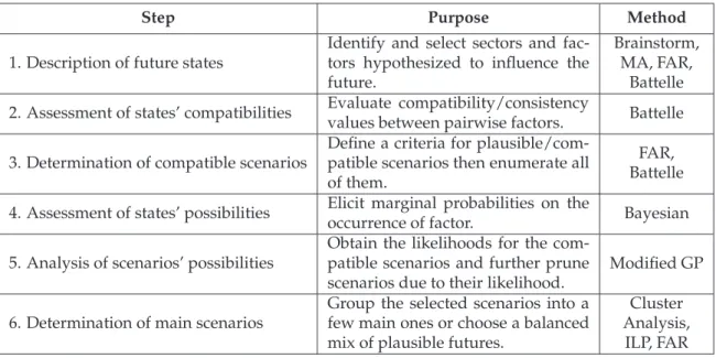
Table 12:Six-step Approach of Combining Methods
Step Purpose Method
1. Description of future states
Identify and select sectors and fac-tors hypothesized to influence the future.
Brainstorm, MA, FAR,
Battelle 2. Assessment of states’ compatibilities Evaluate compatibility/consistency
values between pairwise factors. Battelle 3. Determination of compatible scenarios
Define a criteria for plausible/com-patible scenarios then enumerate all of them.
FAR, Battelle 4. Assessment of states’ possibilities Elicit marginal probabilities on the
occurrence of factor. Bayesian
5. Analysis of scenarios’ possibilities
Obtain the likelihoods for the com-patible scenarios and further prune scenarios due to their likelihood.
Modified GP
6. Determination of main scenarios
Group the selected scenarios into a few main ones or choose a balanced mix of plausible futures.
Cluster Analysis,
ILP, FAR
Table 13:Australia’s Regional Environment in 2030: A Morphological Analysis
Political Governance
P1: Political stability in most
regions P2: Unstable political environment P3: Collapse or change in major players Economic Growth
E1: Developing E2: Declining E3: Collapse
Social Cohesion S1: Tolerance between groups S2: Factionalisation between groups
S3: Conflict and uprising
between group Implications of S&T T1: Overwhelming rate of change or development of technology T2: Continuing (comparable) advancement of technology T3: Lagging advancement of technology. Health and Habitat
H1: Improving/Sustainable H2: Degradation H3: Collapse, meltdown
Type of Operation required by ADF A1: Peacekeeping/Peace
enforcement ADF role
A2: Counter Insurgency/Counter Terrorism A3: Conventional warfare A4: Humanitarian assistance ADF Concurrent Obligations C1: Minor commitment to regional Operations C2: Major commitment to regional Operations C3: Commitment to
Operations further afield
6.2.1 Description of Future States
The first step in developing scenarios is to identify sectors hypothesized to influence the future of the environmental subsystems investigated. Although the number of sectors should be kept to a minimum, the selected sectors need to be comprehensive enough to reflect all relevant concerns about the future and be thoroughly defined so that all experts
understand relevant assumptions. Six to seven is usually recommended for the number of sectors.
Two to five possible future factors are designated by Subject Matter Experts (SME) for each sector using historical trends, current conditions, and expert opinion. These factors are mutually exclusive and technically exhaustive; in other words, other factors were thought to have a probability of occurrence so low as to justify their exclusion.
For the illustrative example, Australia’s Regional Environment in 2030, the description of future states is given in Table 13. The symbolic name is chosen asPESTHACfrom the 7 sectors (listed in the far left boxes). Each sector has 3 factors except Sector A(Type of Operation required by ADF) which has 4.
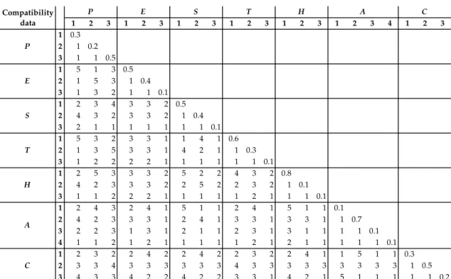
6.2.2 Assessment of States’ Compatibilities
The interdependencies between factors is considered in this step. According to the Battelle approach (Section 3.3), compatibility ratings, kij, are given by asking experts to
evaluate how compatible two factors are.
Table 14:Sample Data
1 2 3 1 2 3 1 2 3 1 2 3 1 2 3 1 2 3 4 1 2 3 1 0.3 2 1 0.2 3 1 1 0.5 1 5 1 3 0.5 2 1 5 3 1 0.4 3 1 3 2 1 1 0.1 1 2 3 4 3 3 2 0.5 2 4 3 2 3 3 2 1 0.4 3 2 1 1 1 1 1 1 1 0.1 1 5 3 2 3 3 1 1 4 1 0.6 2 1 3 5 3 3 1 4 2 1 1 0.3 3 1 2 2 2 2 1 1 1 1 1 1 0.1 1 2 5 3 3 3 2 5 2 2 4 3 2 0.8 2 4 2 3 3 3 2 2 5 2 2 3 2 1 0.1 3 1 1 2 2 2 1 1 1 1 1 2 1 1 1 0.1 1 2 4 3 2 4 1 5 1 1 2 4 1 5 1 1 0.1 2 4 2 3 3 3 1 2 4 1 3 3 1 3 3 1 1 0.7 3 2 2 3 1 3 1 2 1 1 2 3 1 3 1 1 1 1 0.1 4 1 1 2 1 2 1 1 1 1 1 2 1 2 1 1 1 1 1 0.1 1 2 3 2 2 4 2 2 4 2 2 3 2 2 4 1 1 5 1 1 0.3 2 3 3 4 3 3 3 3 3 3 4 3 3 3 3 3 3 3 3 3 1 0.5 3 4 3 3 4 2 2 4 2 2 3 3 1 4 2 1 5 1 1 1 1 1 0.2 Compatibility data C P E S T H A H A C P E S T
For instance, the compatibility data5(below the diagonal) used to illustrate the approach
is presented in Table 14 with:
• a list of all factors i (i = 1, . . . , 22) corresponding to P1, P2, . . . ,C2 and C3
respectively
• the compatibility ratingskij for every two factorsiandj, wherekij ∈ {1, 2, 3, 4, 5}.
Note that the values on the diagonal (e.g. p(E1) = 0.5) are the estimated probabilities
p(i)for the individual factoriwhich will be described in Step 4 (Section 6.2.4). 6.2.3 Determination of Compatible Scenarios
The number of scenarios are exponentially growing with the number of factors. Some combinations of factors may not represent plausible scenarios. In order to decrease the complexity of computation and consider the real situations, the number of scenarios are selected by the following rules:
1. A compatibility rating between any two factors in a scenario must be different to 1 (not likely to occur together),and
2. The average of individual compatibilities between the factors in each scenario is greater than or equal to a lower limitL,orthe number of compatibility ratings of 2 (low likelihood of occurring together) in a scenario is less than or equal to an upper limitU, where
• Lshould be chosen to assure the remaining scenarios had an average scenario compatibility above 3 (in other words, above a neutral compatibility).
• Ushould be below half the number of the sectors in a scenario.
Under these two conditions, scenarios deemed to have a very low possibility of occurring are eliminated. In some cases, the participants have the option to further prune to a subset of these compatible scenarios or to also reintroduce any especially interesting scenarios which were excluded due to their incompatibility.
In the illustrative example, all compatible scenarios (i.e. those without a value of 1) are selected using the following value of LandU:
• Minimum average compatibility value,L=3.285.
• Maximum number of “2 ” ratings,U=3.
Using the DST, the result of this selection process is shown in Table 15 where the ‘Factor’ column lists all accepted scenarios (e.g. Scenario 6: P2E2S1T2H1A1C3).
Table 15:Selected Compatible Scenarios
Factor Factor P E S T H A C P E S T H A C 1 1 1 2 1 1 2 1 6 3.286 18 3 1 1 2 1 1 3 1 3.714 2 1 1 2 1 1 2 2 2 3.381 19 3 1 1 2 1 2 2 1 3.286 3 1 1 2 1 2 2 1 4 3.524 20 3 1 1 2 2 2 2 2 3.143 4 1 1 2 1 2 2 2 1 3.524 21 3 1 2 1 1 2 2 3 3.095 5 2 2 1 2 1 1 2 0 3.667 22 3 1 2 1 2 2 2 3 3.143 6 2 2 1 2 1 1 3 1 3.810 23 3 1 2 2 1 2 2 3 3.048 7 2 2 1 2 1 2 1 4 3.286 24 3 1 2 2 2 2 2 2 3.190 8 2 2 1 2 1 2 2 2 3.238 25 3 2 1 2 1 1 2 0 3.619 9 2 2 1 2 1 3 2 2 3.238 26 3 2 1 2 1 1 3 1 3.714 10 2 2 2 1 1 2 1 4 3.333 27 3 2 1 2 1 2 2 1 3.286 11 2 2 2 1 1 2 2 2 3.286 28 3 2 1 2 1 3 2 1 3.286 12 2 2 2 1 2 2 1 4 3.333 29 3 2 1 2 2 2 2 2 3.143 13 2 2 2 1 2 2 2 3 3.190 30 3 2 2 1 1 2 2 3 3.095 14 2 2 2 2 1 2 2 3 3.095 31 3 2 2 1 2 2 2 3 3.143 15 2 2 2 2 2 2 1 3 3.333 32 3 2 2 2 1 2 2 3 3.048 16 2 2 2 2 2 2 2 3 3.095 33 3 2 2 2 2 2 1 3 3.333 17 3 1 1 2 1 1 2 1 3.524 34 3 2 2 2 2 2 2 2 3.190 N u n b er o f R a ti n g 2 S ce n a ri o A v ea rg e C o m p a ti b il it y V a lu e S ce n a ri o N u n b er o f R a ti n g 2 A v ea rg e C o m p a ti b il it y V a lu e
6.2.4 Assessment of States’ Possibilities
This approach also requires marginal probabilities p(i) on the occurrence of Factors i. Because possible future states of each sector are considered to be exhaustive and mutually exclusive, the assigned marginal probabilities of each factors in each sector sum to 1. Also every sector usually only has 2 to 5 factors, these probabilities are quite easy to elicit. The marginal probabilities and compatibility ratings obtained above are then used to estimate the joint probabilities between two factors and to serve as the basis to obtain cross-impact analysis and conduct the generation of scenarios.
We will use the values on the diagonal of Table 14 as the marginal probabilities for the illustrative example.
6.2.5 Analysis of Scenarios’ Possibilities
We now calculate the probabilities of the scenario selected in the previous step using the modified goal programming formulation (5.1). Here, the DST will call the external
CPLEX solver to find a solution for the modified GP (3a)–(3h) which is modelled through AMPL language.
Table 16:Scenarios Probabilities
S ce n a ri o P ro b a b il it y S ce n a ri o P ro b a b il it y S ce n a ri o P ro b a b il it y S ce n a ri o P ro b a b il it y 1 5.90% 10 5.31% 19 8.85% 28 1.77% 2 8.55% 11 5.31% 20 0.00% 29 0.00% 3 3.24% 12 0.00% 21 6.49% 30 6.49% 4 2.95% 13 0.00% 22 2.95% 31 2.65% 5 2.95% 14 1.18% 23 1.18% 32 1.18% 6 2.36% 15 0.00% 24 1.18% 33 1.18% 7 3.54% 16 0.00% 25 2.95% 34 1.18% 8 3.54% 17 2.36% 26 2.36% 9 1.77% 18 2.36% 27 8.26%
Based on the solution of this modified GP, the upper and lower bounds for all selected scenario probabilities are then obtained by re-solving the modified GP with new objective functions (4) with one extra constraint (5). The arithmetic mean of these probabilities is calculated and shown in Table 16.
Note that Scenario 12, 13, 15, 16, 20 and 29 were computed to have probability 0 throughout the parametric analysis, this is strong indication of these scenarios being implausible. So, subject to expert commentary, these scenarios could be omitted from further consideration.
6.2.6 Determination of Main Scenarios
In the final step, the DST is used again to perform a cluster analysis (Section 5.2) for choosing representative scenarios or to solve ILP’s (Section 5.3) for a balanced mix of plausible scenarios.
Table 17:Sample of Cluster Analysis
Cluster Scenario Average Compability Value Probability 1 1, 4, 5, 7, 8, 9, 10, 14, 17, 18, 19, 21, 22, 23, 24, 25, 27, 28, 30, 31, 32, 34 3.280 77.0% 2 2, 26, 33 3.480 12.1% 3 3, 6, 11 3.440 10.9%