Feature selection for EEG Based biometrics

저작자표시-비영리-변경금지 2.0 대한민국 이용자는 아래의 조건을 따르는 경우에 한하여 자유롭게 l 이 저작물을 복제, 배포, 전송, 전시, 공연 및 방송할 수 있습니다. 다음과 같은 조건을 따라야 합니다: l 귀하는, 이 저작물의 재이용이나 배포의 경우, 이 저작물에 적용된 이용허락조건 을 명확하게 나타내어야 합니다. l 저작권자로부터 별도의 허가를 받으면 이러한 조건들은 적용되지 않습니다. 저작권법에 따른 이용자의 권리는 위의 내용에 의하여 영향을 받지 않습니다. 이것은 이용허락규약(Legal Code)을 이해하기 쉽게 요약한 것입니다. Disclaimer 저작자표시. 귀하는 원저작자를 표시하여야 합니다. 비영리. 귀하는 이 저작물을 영리 목적으로 이용할 수 없습니다. 변경금지. 귀하는 이 저작물을 개작, 변형 또는 가공할 수 없습니다.

Master's Thesis

Feature selection for EEG Based biometrics

Chungho Lee

Department of Human Factors Engineering

Graduate School of UNIST

2017

Feature selection for EEG Based biometrics

Chungho Lee

Department of Human Factors Engineering

Feature selection for EEG Based biometrics

A thesis/dissertation

submitted to the Graduate School of UNIST

in partial fulfillment of the

requirements for the degree of

Master of Science

Chungho Lee

11. 29. 2017 Month/Day/Year of submission

Approved by

_________________________

Advisor

Sung-Phil Kim

Feature selection for EEG Based biometrics

Chungho Lee

This certifies that the thesis/dissertation of Chungho Lee is approved.

11/29/2016

signature

___________________________

Advisor: Prof. Sung-Phil Kim

signature

___________________________

Prof. Sung-Phil Kim

signature

___________________________

Prof. Ian Oakley

signature

___________________________

Prof. Se Young Chun

I

ABSTRACT

EEG-based biometrics identify individuals by using personal and distinctive information in human brain. This thesis aims to evaluate the electroencephalography (EEG) features and channels for biometrics and to propose methodology that identifies individuals. In my research, I recorded fourteen EEG channel signals from thirty subjects. While record EEG signal, subjects were asked to relax and keep eyes closed for 2 minutes. In addition, to evaluate intra-individual variability, we recorded EEG ten times for each subject, and every recording conducted on different days to reduce within-day effects. After acquisition of data, for each channel, I calculated eight features: alpha/beta power ratio, alpha/theta power ratio, beta/theta power ratio, median frequency, PSD entropy, permutation entropy, sample entropy, and maximum Lyapunov exponents. Then, I scored 112 features with three feature selection algorithms: Fisher score, reliefF, and information gain. Finally, I classified EEG data using a linear discriminant analysis (LDA) with a leave-one-out cross validation method. As a result, the best feature set was composed of 23 features that highly ranked on Fisher score and yielded a 18.56% half total error rate. In addition, according to scores calculated by feature selection, EEG channels located on occipital and right temporal areas most contributed to identify individuals. Thus, with suggested methodologies and channels, implementation of efficient EEG-based biometrics is possible.

II

List of Publications

This thesis is based on the works recorded below. Especially, the main idea of this thesis is in a course of preparation for a publishing.

Conferences Proceedings and abstracts

1. Lee, C., Kang, J, H., & Kim, S. P.. (2016). Feature selection using mutual information for EEG based biometrics. In Telecommunications and Signal Processing (TSP), 2016 39th International Conference. IEEE.

III

Contents

1. Introduction ---1

1.1 Introduction to biometrics--- 2

1.2 Introduction to EEG--- 4

1.3 EEG based biometrics--- 5

1.4 Research aim--- 5

2. Experimental Design--- 6

2.1 Participants and ethics approval--- 7

2.2 Data acquisition---7 2.3 Experimental procedure --- 7 3. Data Analysis--- 9 3.1 Preprocessing--- 10 3.2 Feature extraction--- 10 3.3 Feature selection--- 12 3.4 Verification--- 15

IV 4. Results--- 16 3.1 Feature selection--- 17 3.2 Verification--- 17 5. Discussion---22 5.1 General discussion--- 23

5.2 Feature selection score--- 23

5.3 Limitations and future works --- 24

V

List of Figures

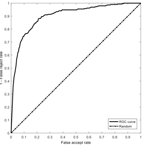
Figure 1. Example of ROC curve --- 3

Figure 2. Names and positions of international 10-20 system (Oostenveld & Praamstra 2001) --- 4

Figure 3. (A) Experimental environment, (B) Emotiv EPOC headset on a subject, (C) Names and positions of Emotiv EPOC electrodes, (D) Experimental procedure. The eye close sign and first beep sound triggered by moderator--- 8

Figure 4. (A) Fisher scores in fourteen EEG channels, (B) Fisher scores in feature eight feature groups, (C) ReliefF score in fourteen EEG channels, (D) ReliefF score in feature eight feature groups, (E) Information gain in fourteen EEG channels, (F) Information gain in feature eight feature groups--- 18

Figure 5. Topograph of feature selection scores--- 18

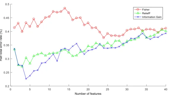
Figure 6. Half total error rate versus number of features--- 20

Figure 7. Area under the ROC curve versus number of features--- 20

VI

List of Tables

VII

List of Equations

１

２ 1.1 Introduction to biometrics

1.1.1 Personal identification

Personal identification is associating an identity with an individual (Jain et al. 2006). Depending on the purpose, personal identification problems can be categorized as two types: verification and recognition (Jain et al. 2006). A verification problem confirms or denies a given identity. A recognition problem establishes identity from a set of identities. In this study, since we do not consider the recognition problem, personal identification only will represent the verification problem. Existing personal authentication techniques are based on three types of methodologies: what you have, what you know, and biometric characteristics (Ratha et al. 2001). Personal identification systems based on a subject's possessions identify individuals by checking keys, such as a car key, id card, or even a credit card. Some personal identification systems use what you know, such as general log-in systems, using personal identification numbers (PINs) that belongs to the case (Miller 1994). However, these two types of identification systems pose a danger, in that a key or other item can be lost or overlooked. They can also be easily compromised by someone who with malice may want to hide an identity. Therefore, the biometric system of personal identification was created, based on personal characteristics

1.1.2 Biometric identifiers

The biometric system identifies individuals based on the individual's physical, chemical, or behavioral characteristics (Jain et al. 2007). Biometric characteristics, also called biometric identifiers, follow four requirements: (i) universality, (ii) distinctiveness, (iii) permanence, and (iv) collectivity (Jain et al. 2007). First, to satisfy universality, every person should possess the proper characteristics. Second, the characteristics of each person should be different enough to be measurable. Third, over a period of time, the degree of change in the individual's characteristics should be below a certain level. Fourth, these characteristics should be quantitatively measurable (Alice 2003). It should be especially noted that distinctiveness represents inter-subject variability, and permanence represents intra-subject variability. For a reliable biometric system, intra-subject variability should be less then inter-subject variability.

Currently, there are five typical biometric identifiers: fingerprints, face recognition, hand geometry, the iris, and the voice (Alice 2003). In terms of universality and collectivity, all five identifiers are reasonable indicators. In terms of distinctiveness on the other hand, while fingerprints, hand geometry, and the iris show reasonable distinctiveness and permanence, the voice is not a reliable biometric identifier since even a slight cold can change the quality of one's voice. In face recognition, permanence rates fair, but distinctiveness is relatively low.

３ 1.1.3 Performance measure of biometric system

For each attempted identification, the biometrics system can result in either acceptance or rejection, and acceptance and rejection can be either true or false. Thus, the results from the biometric system can be represented by two types of error rates, the false accept rate (FAR) and the false reject rate (FRR). In most cases, there is a trade-off between the FAR and the FRR. By using the receiver operating characteristic (ROC) curve, the trade-off between the FAR and the FRR can be seen (Figure 1). From the ROC curve, we can calculate the area under the curve (AUC), and the equal error rate (EER), the error rate when the FAR is equals to the FRR. In general, the higher AUC, and the lower EER represent a more reliable biometric system. For the biometric systems that apply the multiple attempts scenario, the false match rate (FMR), and the false non-match rate (FNMR) generally refer to performance. (Jain et al. 2011). However, in this study, we only consider the biometric systems that do not allow for multiple attempts.

４ 1.2 Introduction to EEG

Electroencephalography is one of the methodologies that measuring the brain activity. When electric state of neurons changed, tiny electromagnetic field is evoked. To measure the electromagnetic field evoked by neurons, electroencephalography measures electric potential between ground and target electrode on scalp (Nunez et al. 2006). However, since electric potential evoked by neurons is very low, signal-noise ratio of EEG is relatively low. Also, our skull and scalp act as capacitor, only low frequency signal are observed on the scalp (Ramon et al. 2009). Despites of this disadvantages, EEG have been used for some reasons. First, temporal resolution of EEG is relatively high. Second, scalp EEG is non-invasive method, and EEG device is relatively easy to record. Third, scalp EEG device is relatively easy to commercialize, and adopt to wearable devices. Thanks to these advantages, lots of commercialized EEG devices are emerged.

To describe the location of EEG electrodes, the International 10-20 system is widely used. Each electrode has letters of brain lobe, and number to describe the location from left to right. There are five letters generally used: ‘F’ (frontal), ‘T’ (temporal), ‘C’ (central), ‘P’ (parietal), and ‘O’ (occipital). The small ‘p’ represents the polar, and ‘A’ represents the anterior part of brain area. The numbers increase according to the distance from the center line, from inion to nasion. In addition, small ‘z’ represents the zero.

５ 1.3 EEG based biometrics

As a relatively inexpensive methodology to observe the human brain, EEG-based biometric systems have been developed by a number of studies (Del Pozo-Banos et al. 2014). In the development of these systems, few studies used the dataset of BCI Competition 2003 IIIa. By using multiple features, including AR coefficients, linear complexity, energy spectral density, and phase synchronization, this biometric system identified three subjects with 82% accuracy (Bao et al. 2009). Using the same dataset, another study reported 83.9% (Hu 2009). A study using the dataset of the BCI Competition of 2005 IIIa, and 2008 A, B reported authentication performance of 99%, 46.24%, and 80.8%, respectively, for the datasets (Nguyen et al. 2012). There have been few studies using visual-evoked potentials for the biometric system. Ravi and Palaniappan authenticated 20 subjects with 95% accuracy using 61-channel EEG data recorded for visual-evoked potentials (Ravi & Palaniappan 2005). Palaniappan and Mandic later improved accuracy to 98% with 40 subjects (Palaniappan & Mandic 2007). Resting state EEG signals have also been employed for biometric authentication. With an 8-channel EEG signal recorded during the resting state, one study identified 40 subjects with 85% accuracy (Paranjape et al. 2001). In another study, a 2-channel EEG signal during the resting state, with eyes closed authenticated 23 subjects with 30% EER (Miyamoto et al. 2009). By using the same dataset, other studies reported 11% EER (Nakanishi et al., 2009).

1.4 Research aim

The purpose of this study is to compare the electroencephalogram features for biometric identification and propose a methodology for the identification of individuals. To achieve this, we recorded electroencephalogram signals ten times for each of 30 subjects with a 14-channel Emotive EPOC EEG device. For each channel, we calculated eight features: alpha/beta power ratio, alpha/theta power ratio, beta/theta power ratio, median frequency, PSD entropy, permutation entropy, sample entropy, and maximum Lyapunov exponents. Then, we scored 112 features with three feature selection algorithms: Fisher score, reliefF, and information gain. Finally, we classified recordings with linear discriminant analysis (LDA) with selected features set.

６

2. Experimental

Design

７ 2.1 Participants and ethics approval

Thirty healthy subjects participated in this study (20 males, 10 females, 24.9 +- 4.33 years old). Participants had no history of neurological disorders or deficits. The study was approved by the ethical committee of Ulsan National Institute of Science and Technology (UNISTIRB-16-01-G).

2.2 Data acquisition

EEG data were recorded by using the portable Emotive EPOC device with 14 semi-dry electrodes (Figure 3.A, Figure 3.B). EEG signals were digitized at a 128 Hz sampling rate and reference electrodes were located at P3 and P4. For analysis, 14 EEG channels (AF3, AF4, F3, F4, F7, F8, FC5, FC6, O1, O2, P7, P8, T7, T8) were used (Figure 3.C). For the multimodal biometric system, the electrocardiogram (ECG) signal was recorded just before and just after the EEG recording. However, this study only covers the EEG-based biometric system.

2.3 Experimental procedure

Before recording EEG signals, the subjects asked to sit on an office chair in an electrically shielded room and stay relaxed. While recording the EEG signal, the subjects were instructed to keep their eyes closed until a beep sounded (Figure 3.D). The EEG signal recorded for 2 minutes, and each subject was required to repeat the recording 10 times on different days. However, because of technical problems, only 289 recordings available for analysis.

８

Figure 3. (A) Experimental environment, (B) Emotiv EPOC headset on a subject, (C) Names and positions of Emotiv EPOC electrodes,

９

１０ 3.1 Preprocessing

Before calculation, the EEG signals were filtered by a finite impulse response (FIR) band-pass filter with a frequency range from 2 to 50Hz. For feature extraction, filtered EEG signals were segmented into two-seconds epoch. From each recording, 20 epochs were randomly selected between artifact-free epochs. Through each feature extraction algorithm, one scalar value was obtained from each epoch. Through this extraction process, 289 by 20 by 8 sized feature matrixes (289 recordings, 20 epochs, 8 features) were extracted.

3.2 Feature extraction

3.2.1 Power Spectral Density (PSD)

For each epoch, we obtained power spectral density (PSD) by using a fast Fourier transform. By the FFT method, a Hamming window was adopted and zero padded to set the number of FFT points to

the power of two. PSD was obtained by autoregressive (AR) coefficients. Where am is

autoregressive coefficient obtained by using the Yule-Walker method, power spectral density is given as 𝑆𝐴𝑅(𝑓) = 𝜎𝑒2 |1 + ∑𝑀𝑚=1𝑎𝑚𝑒(−𝑗2𝜋𝑓𝑚∆𝑡|2 (3.1) (Akay 2012)

Here, 𝑀 is order of AR filter order, ∆𝑡 is sampling interval, and 𝜎𝑒2 is noise power.

From PSD data, power was adjusted to theta (2~7Hz), alpha (7~13Hz), and beta (13~20Hz). ‘Theta/beta’, ‘alpha/beta’, and ‘alpha/theta’ power ratios were then calculated. Also, median frequency and Shanon entropy of PSD were calculated.

１１ 3.2.2 Sample entropy

Let X = {𝑥1, 𝑥2, … , 𝑥𝑁} be the time-series vector, and X𝑚(𝑖) = {𝑥𝑖, 𝑥𝑖+1, … , 𝑥𝑖+𝑚−1} the sub-vector

of X with length m. Then, we can define 𝐴, 𝐵, sample entropy (Lake et al. 2002).

𝐴 = number of pairs that dist[X𝑚+1(𝑖), X𝑚+1(𝑗)] < 𝑟

𝐵 = number of pairs that dist[X𝑚(𝑖), X𝑚(𝑗)] < 𝑟

𝑆𝑎𝑚𝑝𝑙𝑒 𝐸𝑛𝑡𝑟𝑜𝑝𝑦 = − log𝐴

𝐵 (3.2)

Sample entropy is defined as “the negative natural logarithm of the conditional probability that two sequences similar for m points remain similar at the next point” (Richman & Moorman 2000). To determine the conditional probability, every possible pair of sub-vectors is checked for whether the distance falls within the threshold range. If the time-series signal is composed of a single pattern, conditional probability will become one. In other words, the sample entropy of a perfectly regular signal is zero.

3.2.3 Permutation entropy

Similarly, let X = {𝑥1, 𝑥2, … , 𝑥𝑁} be the time-series vector, and X𝑚(𝑖) = {𝑥𝑖, 𝑥𝑖+1, … , 𝑥𝑖+𝑚−1} the

sub-vector of X with length m. Then, let π represent the order of elements of X𝑚. For instance, if

m=2, the number of π is two: 𝑥1> 𝑥2, 𝑥2> 𝑥1. Then, we can define permutation entropy (Bandt et

al. 2002).

𝐻(𝑛) = − ∑ 𝑝(𝜋) log2𝑝(𝜋) (3.3)

Where

𝑝(𝜋) = 𝑛𝑢𝑚𝑏𝑒𝑟 𝑜𝑓 𝑋𝑚 ℎ𝑎𝑠 𝑡𝑦𝑝𝑒 𝜋

𝑁 − 𝑚 + 1 (3.4)

Permutation entropy explains the probability distribution of permutations. If a time-series signal is perfectly un-regular, the probability of permutations will be equally distributed, and permutation entropy will be maximized. In contrast, as a time-series signal is regularized, the permutation entropy will decrease.

１２ 3.2.4 Lyapunov exponents

The Lyapunov exponent quantifies the rate of separation of close trajectories. If 𝛿𝑖(𝑡) is the distance

between two trajectories in i-th dimension of state space when time is t, the Lyapunov exponent is defined as the average growth rate of the distance. (Kantz et al. 2004, Wolf et al. 1985)

λi= lim 𝑥→∞ 1 𝑡log2 ‖𝛿𝑥𝑖(𝑡)‖ ‖𝛿𝑥𝑖(0)‖ (3.5)

As the Lyapunov exponent is related to expansion or contraction in phase space, it is widely used to quantify chastity. For computation of the maximum Lyapunov exponent, we embedded an EEG signal into three dimensions, with a time delay of one second.

3.3 Feature selection 3.3.1 Fisher score

The Fisher score can be computed by the mean and variance of each group.

Where 𝑢 = 𝑜𝑣𝑒𝑟𝑎𝑙𝑙 𝑚𝑒𝑎𝑛 𝑢𝑘 = 𝑚𝑒𝑎𝑛 𝑜𝑓 𝑡ℎ𝑒 𝑘 − 𝑡h 𝑔𝑟𝑜𝑢𝑝 𝜎_𝑘2= 𝑣𝑎𝑟𝑖𝑎𝑛𝑐𝑒 𝑜𝑓 𝑡ℎ𝑒 𝑘 − 𝑡h 𝑔𝑟𝑜𝑢𝑝 𝑛𝑘 = 𝑛𝑢𝑚𝑏𝑒𝑟 𝑜𝑓 𝑡ℎ𝑒 𝑘 − 𝑡h 𝑔𝑟𝑜𝑢𝑝 𝐹𝑖𝑠ℎ𝑒𝑟 𝑠𝑐𝑜𝑟𝑒 =∑ 𝑛𝑘(𝑢𝑘− 𝑢) 2 ∑ 𝑛𝑘𝜎𝑘2 (3.6) (Gu et al. 2012)

While the numerator of the Fisher score represents how each group is separated from other groups, the denominator of the Fisher score indicates how precise each group is. Thus, as variability between groups is large, and variability of each group is small, the Fisher score will increase.

１３ 3.3.2 ReliefF

Relief, the binary form of ReliefF, is calculated by finding the closest intra-class and the inter-class instances, called ‘near-miss’ and ‘near-hit’. This algorithm repeats finding ‘near-hit’ and ‘near-miss’ and updates the weight vector according to an update rule (Kira et al. 1992).

𝑊𝑖 = 𝑊𝑖− (𝑥𝑖− 𝑛𝑒𝑎𝑟𝐻𝑖𝑡𝑖)2+ (𝑥𝑖− 𝑛𝑒𝑎𝑟𝑀𝑖𝑠𝑠𝑖)2

At the beginning of iteration, the weight vector starts with zeros. Then, for each iteration, the update rule updates the weight vector with a Euclidian distance. As near-hit is close to the given sample, and near-miss is far from the given sample, the weight vector will be maximized. The number of iterations is one of the parameters that needs to be specified.

On the other hand, ReliefF is the advanced form of Relief. In contrast with Relief, ReliefF finds multiple near-hits and near-misses from each class and averages them to update the weight vector. As a result, ReliefF extends Relief to multi-class problem, and solves noisy instances (Robnik-Šikonja et al. 1997).

１４ 3.3.3 Information gain

The information gain of term t can be defined by the sum of entropy.

𝐺(𝑡) = − ∑ 𝑝(𝑐𝑖) log 𝑝(𝑐𝑖)

+𝑝(𝑡) ∑ 𝑝(𝑐𝑖|𝑡) log 𝑝(𝑐𝑖|𝑡)

+𝑝(𝑡̅) ∑ 𝑝(𝑐𝑖|𝑡̅) log 𝑝(𝑐𝑖|𝑡̅)

(3.7)

(Yang et al. 1997)

For the multi-class classification problem, the information gain 𝐺𝑎𝑖𝑛(𝑆, 𝐴) of an attribute 𝐴,

collection of examples 𝑆 is defined as

𝐺𝑎𝑖𝑛(𝑆, 𝐴) ≡ 𝐸𝑛𝑡𝑟𝑜𝑝𝑦(𝑆) − ∑ |𝑆𝑣|

|𝑆| 𝐸𝑛𝑡𝑟𝑜𝑝𝑦(𝑆𝑣)

𝑣∈𝑉𝑎𝑙𝑢𝑒𝑠(𝐴)

(3.8)

(Mitchell 1997)

The first term of information gain is typical entropy of collection. On the other hand, second term is

expected entropy of collections for each value 𝑣. Thus, the information gain is the expected reduction

of entropy by knowing the attribute 𝐴 (Mitchel 1997). If attribute 𝐴 represents the set of samples

１５ 3.4 Verification

For verification of given matrixes, we calculated the logarithm of likelihood that can be obtained by linear discriminant analysis (LDA). If the calculated log likelihood was larger than the threshold, the given feature vector was accepted, if smaller than threshold, the given vector was rejected. The threshold set to the value makes FAR and FRR equal. The verification process was tested with two scenarios. First, we tested the verification process with the ordinary leave-one-out method. For each recording, we made a model by using the other recordings as training data, and tested for a single recording. In this test, one subject was set to genuine, other subjects were set to imposters, and then the whole process was repeated by changing the genuine.

The second test scenario followed flow of time. We set the initial training data. Initial training data contained the first three records of genuine, and the complete data of the other subjects, except the imposters. With initial training data, we verified one record of genuine, and one record of imposter. The next training data contained initial training data and accepted training data. The number of genuine records in the initial training data was set to the minimum amount of data necessary to build the model. Imposters were fixed to subject number 4 and 5. Since the number of records of these two subjects were too small, we excluded them from the test, and assigned them to the imposters.

１６

１７ 4.1 Feature selection

By means of the feature selection algorithms, we sorted features with scores (Figure 4). To perform statistical analysis of the feature selection, Wilcoxon's signed-rank test was conducted between groups of features. In the case of the Fisher score, O1 and O2 showed the highest score. A score of O2 was slightly higher than that of O1, but not significant. Comparing to O2, eight EEG channels were significantly different: F4 (𝑝 < 0.02), FC6 (𝑝 < 0.02), F3 (𝑝 < 0.02), FC5 (𝑝 = 0.02), AF3 (𝑝 = 0.02), P7 (𝑝 < 0.01), P8 (𝑝 < 0.01), and F7 (𝑝 < 0.01). Among the eight feature groups, the alpha and beta power ratio showed the best score. The alpha and beta power ratio score were significantly higher than other features groups (𝑝 < 0.01). The result of ReliefF was almost same as the Fisher score. However, the best channel was O1, not O2, and the score of O1 was significantly higher than five EEG channels: AF4 (𝑝 = 0.04), AF3 (𝑝 < 0.01), FC5 (𝑝 < 0.01), F7 (𝑝 < 0.01), and P7 (𝑝 < 0.01). Results of information gain was also similar to the two algorithms, but slightly different. Among EEG channels, O1 showed the best score, and significantly higher than the five EEG channels, AF4 (𝑝 = 0.04), AF3 (𝑝 < 0.01), FC5 (𝑝 < 0.01), F7 (𝑝 < 0.01), and P7 (𝑝 < 0.01).

Generally, scores of the right hemisphere were much higher than that of left hemisphere (Figure 5). For three feature selection scores, there were significant differences between scores of the right and left hemispheres (𝑝 < 0.01).

4.2 Verification

4.2.1 Leave-one-out test

To evaluate performance, we conducted verification with a feature set composed of highly ranked features. To calculate the optimal number of features, we conducted verifications while varying the number of features (Figure 6). To compare the performance models, we repeated this process with randomly generated scores for twenty times. As a result, the half total error rate of feature selection algorithms was significantly lower than randomly ordered features when the number of features were small. In the case of the Fisher score and ReliefF algorithms, p-value exceeded 0.05 first when n=40. With the information gain algorithm, p-value was not to exceed 0.01 until n=65. According to HTER, the best feature combination was 23 features that ranked highly on the Fisher score (HTER=18.56%). To show the performance clearly, we calculated the area under the ROC curve (Figure 7). The area under the ROC curve from feature selection algorithms remained a significantly higher value than that of the random order, and p value exceeded 0.05 first when n=35, 40, 35 for each Fisher score, ReliefF, information gain algorithm.

１８

Figure 4. (A) Fisher scores in fourteen EEG channels, (B) Fisher scores in feature eight feature groups, (C) ReliefF score in fourteen EEG channels, (D) ReliefF score in feature eight feature groups, (E) Information gain in fourteen EEG channels, (F) Information gain in feature eight feature groups

１９

Rank Fisher score ReliefF Information gain Feature Name Channel Score Feature Name Channel Score Feature Name Channel Score 1 Entropy O1 2.3180 Alpha/Beta O1 0.1176 Alpha/Beta O1 1.2064 2 Alpha/Beta O1 2.1357 Entropy O1 0.1103 Entropy O1 1.1602 3 Alpha/Beta AF4 2.0501 Entropy O2 0.0912 Median P8 1.1195 4 Alpha/Beta F8 1.9254 Alpha/Beta AF4 0.0835 Entropy O2 1.1189 5 Alpha/Beta T8 1.8932 Alpha/Beta O2 0.0827 Alpha/Beta F8 1.0676 6 Median O2 1.8791 Alpha/Beta T8 0.0784 Alpha/Beta T8 1.0603 7 Alpha/Beta AF3 1.7592 Alpha/Beta F8 0.0767 Alpha/Beta AF4 1.0577 8 Alpha/Beta FC6 1.7311 PermEn O1 0.0756 Alpha/Beta FC6 1.0574 9 Entropy O2 1.7100 Alpha/Beta F3 0.0754 Alpha/Beta F4 1.0377 10 Alpha/Beta O2 1.6835 Alpha/Beta P8 0.0748 Median T8 1.0253 11 PermEn O1 1.6681 Alpha/Beta FC6 0.0746 Alpha/Beta O2 1.0242 12 Alpha/Beta P8 1.5596 Median P8 0.0731 Alpha/Beta P8 1.0077 13 Alpha/Beta F3 1.4974 Alpha/Theta O2 0.0716 Alpha/Beta F3 1.0021 14 Entropy AF4 1.4945 Alpha/Beta F4 0.0713 Median F3 0.9924 15 Alpha/Theta T8 1.4821 Median O2 0.0694 Median F4 0.9866 16 Alpha/Theta O2 1.4799 Alpha/Beta AF3 0.0668 Median O2 0.9822 17 Median T8 1.4448 Entropy AF4 0.0621 Alpha/Beta AF3 0.9746 18 Alpha/Beta F4 1.4439 Alpha/Theta O1 0.0617 PermEn O1 0.9673 19 Median FC6 1.4148 Entropy F3 0.0600 Median AF4 0.9670 20 PermEn O2 1.3910 Alpha/Theta T8 0.0593 Alpha/Theta O1 0.9649 21 Alpha/Theta AF4 1.3638 Median T8 0.0584 Median O1 0.9615 22 Alpha/Beta F7 1.3392 Entropy AF3 0.0582 Alpha/Theta O2 0.9598 23 Alpha/Theta F8 1.3312 Alpha/Theta P8 0.0570 Entropy F3 0.9443 24 Median AF4 1.2471 PermEn O2 0.0569 Median F8 0.9426 25 Median F3 1.2075 Alpha/Beta P7 0.0569 Median AF3 0.9398 26 Median P8 1.1996 Alpha/Beta F7 0.0551 Alpha/Theta FC6 0.9370 27 Entropy F3 1.1705 Median FC6 0.0544 Alpha/Theta T8 0.9370 28 Entropy AF3 1.1474 Median F3 0.0536 Alpha/Theta P8 0.9230 29 Alpha/Theta FC6 1.1260 Median F4 0.0535 Entropy AF4 0.9228 30 Median F4 1.1223 Median AF4 0.0507 Median FC6 0.9211 31 Alpha/Theta P8 1.0907 Alpha/Theta F8 0.0505 PermEn O2 0.9203 32 Alpha/Theta F7 1.0744 Alpha/Theta AF4 0.0504 Alpha/Theta AF4 0.9183 33 Median F8 1.0743 Median F8 0.0499 Entropy AF3 0.9036 34 Alpha/Theta O1 1.0697 Median O1 0.0494 Alpha/Theta F8 0.8776 35 Alpha/Theta AF3 1.0264 Alpha/Theta FC6 0.0491 Alpha/Beta P7 0.8745 36 Entropy FC6 1.0169 Entropy F7 0.0435 Theta/Beta P8 0.8661 37 Alpha/Theta F3 1.0087 Alpha/Theta F3 0.0433 Entropy T8 0.8631 38 Entropy F7 1.0016 Alpha/Beta FC5 0.0427 Alpha/Beta F7 0.8409 39 Median O1 0.9552 Alpha/Theta AF3 0.0421 Median T7 0.8361 40 Alpha/Theta F4 0.9458 Entropy FC6 0.0416 Alpha/Beta T7 0.8350 41 Alpha/Beta P7 0.9317 Alpha/Beta T7 0.0414 Alpha/Theta F4 0.8332 42 Alpha/Beta FC5 0.9290 Entropy T8 0.0408 MaxLyp F4 0.8235 43 Alpha/Theta FC5 0.8982 Alpha/Theta F4 0.0403 Alpha/Theta F3 0.8211 44 Entropy F4 0.8665 Median F7 0.0389 Entropy FC6 0.8194 45 Entropy T8 0.8291 Median AF3 0.0383 Median F7 0.8191 46 Alpha/Beta T7 0.8278 Alpha/Theta F7 0.0381 MaxLyp F3 0.8111 47 Median F7 0.8140 Theta/Beta P8 0.0360 MaxLyp F8 0.8060 48 Entropy FC5 0.7583 Entropy FC5 0.0342 Median FC5 0.8053 49 PermEn F3 0.7506 Alpha/Theta FC5 0.0337 SampEn O1 0.7999 50 Alpha/Theta P7 0.7245 Median T7 0.0330 Alpha/Theta AF3 0.7940 51 Theta/Beta O2 0.7016 SampEn O1 0.0323 MaxLyp P8 0.7914 52 SampEn O1 0.6994 MaxLyp T7 0.0320 SampEn F3 0.7895 53 MaxLyp T7 0.6981 Entropy F8 0.0320 MaxLyp T7 0.7891 54 Median T7 0.6967 Alpha/Theta P7 0.0319 Alpha/Beta FC5 0.7819 55 SampEn T7 0.6762 Entropy F4 0.0318 Entropy F8 0.7811 56 Entropy F8 0.6633 SampEn T7 0.0315 Entropy F7 0.7810

２０

Figure 6. Half total error rate versus number of features

２１ 4.2.2 Adaptive scenario

As a result of the adaptive scenario, recordings of genuines and imposters were verified. The results of the scenario were represented by HTER, man of FAR and FRR. FAR was the error rate for imposters, and FRR was the error rate for genuines. In case of information gain, HTER decreased to 22.66% until the number of features was four, and increased according to the number of features (Figure 8). However, HTER of the ReliefF algorithm increased as number of features. Among three feature selection algorithms, the Fisher score showed the worst results. Since the weights of three features selection algorithms were calculated for each training set, the feature set selected by this scenario should have been different from table 1. When every recording was tested, the best four features selected by information gain were ‘Alpha/Beta’/’O1’, ‘Entropy’/’O1’, ‘Entropy’/‘O2’, ‘Median’/’P8’.

２２

２３ 5.1 General discussion

The result of classification showed that the feature selection algorithms we adopted were proper. Compared to the randomly generated order, results of our feature selection algorithm indicated better performance when the number of features did not exceed 40. By means of Fisher score algorithms, we found a feature set that yielded 18.56% HTER, the best performance of this study.

In the case of the adaptive scenario, the information gain algorithm resulted in far better performance than other algorithms, especially, when the number of features was four. HTER then dropped to 22.66%, even though only three recordings of genuines were included in the initial training data.

5.2 Feature selection score

Although the results of the three feature selection algorithms were slightly different, we still found interesting comparisons.

First, the EEG channels located on the occipital yielded the best performance. Because the subjects were asked to close their eyes while recording, the high score from this region, the alpha and beta power ratio, were in accord with the study on user recognition using the "Eyes Closed Resting Conditions" protocol (Campisi et al. 2011).

We also found that scores of channels located on the right hemisphere scored significantly higher than those on the left hemisphere. Still, a few studies maintain that there is no hemisphere effect (Tangkraingkij et al. 2009). In future studies, we propose to explore the hemisphere effect in biometrics more strictly by controlling factors such as the use of right-handed subjects.

On the other hand, among the eight feature groups, there are features that represent chaosity and complexity, such as sample entropy, permutation entropy, Lyapunov exponent demonstrated relatively low performance. If we consider a study reporting that maximum Lyapunov exponent is a great feature for subject classification, this phenomenon would be hard to accept. However, it can be explained by the noise level of the EEG device. Since we did not use an EEG device for research, the signal-to-noise ratio was relatively low. Even if sample entropy and permutation entropy are relatively robust against noise level (Aboy et al. 2007; Ramdani et al. 2009), these types of features may produce high complexity with an EEG device that has a low signal-to-noise ratio.

２４ 5.3 Limitations and future works

There were a few limitations in this study that should be explored in future work. First, the number of features are not sufficient. With only a few features, results of the comparison between channels are less reliable. To solve this problem, at the minimum, features that are broadly used should be included in future work.

Second, periods of testing were too limited. In this study, we were required to conduct the experiment within 10 days, which was too short a time to observe the tendencies of EEG features. To test the biometric system properly, the period of time between experiments should be increased.

２５

REFERENCES

1. Aboy, M., Cuesta-Frau, D., Austin, D., & Mico-Tormos, P. (2007, August). Characterization of sample entropy in the context of biomedical signal analysis. In 2007 29th Annual International Conference of the IEEE Engineering in Medicine and Biology Society (pp. 5942-5945). IEEE.

2. Akay, M. (2012). Biomedical signal processing. Academic Press.

3. Alice, I. (2003). Biometric recognition: Security and privacy concerns. IEEE Security & Privacy.

4. Bandt, C., & Pompe, B. (2002). Permutation entropy: a natural complexity measure for time series. Physical review letters, 88(17), 174102.

5. Bao, X., Wang, J., & Hu, J. (2009, June). Method of individual identification based on electroencephalogram analysis. In New Trends in Information and Service Science, 2009. NISS'09. International Conference on (pp. 390-393). IEEE.

6. Campisi, P., Scarano, G., Babiloni, F., Fallani, F. D., Colonnese, S., Maiorana, E., & Forastiere, L. (2011, November). Brain waves based user recognition using the “eyes closed resting conditions” protocol. In 2011 IEEE International Workshop on Information Forensics and Security (pp. 1-6). IEEE.

7. Del Pozo-Banos, M., Alonso, J. B., Ticay-Rivas, J. R., & Travieso, C. M. (2014). Electroencephalogram subject identification: A review. Expert Systems with Applications, 41(15), 6537-6554.

8. Gu, Q., Li, Z., & Han, J. (2012). Generalized fisher score for feature selection. arXiv preprint arXiv:1202.3725.

9. Guyon, I., & Elisseeff, A. (2003). An introduction to variable and feature selection. Journal of machine learning research, 3(Mar), 1157-1182.

10. Hu, J. F. (2009, December). New biometric approach based on motor imagery EEG signals. In 2009 International Conference on Future BioMedical Information Engineering (FBIE) (pp. 94-97). IEEE.

２６

11. Jain, A., Bolle, R., & Pankanti, S. (Eds.). (2006). Biometrics: personal identification in networked society (Vol. 479). Springer Science & Business Media.

12. Jain, A., Flynn, P., & Ross, A. A. (Eds.). (2007). Handbook of biometrics. Springer Science & Business Media.

13. Jain, A., Hong, L., & Pankanti, S. (2000). Biometric identification. Communications of the ACM, 43(2), 90-98.

14. Jain, A., Ross, A. A., & Nandakumar, K. (2011). Introduction to biometrics. Springer Science & Business Media.

15. Kantz, H., & Schreiber, T. (2004). Nonlinear time series analysis (Vol. 7). Cambridge university press.

16. Kira, K., & Rendell, L. A. (1992, July). The feature selection problem: Traditional methods and a new algorithm. In AAAI (Vol. 2, pp. 129-134).

17. Lake, D. E., Richman, J. S., Griffin, M. P., & Moorman, J. R. (2002). Sample entropy analysis of neonatal heart rate variability. American Journal of Physiology-Regulatory, Integrative and Comparative Physiology, 283(3), R789-R797.

18. Miller, B. (1994). Vital signs of identity [biometrics]. IEEE spectrum, 31(2), 22-30.

19. Mitchell, T. M. (1997), Machine Learning, McGraw-Hill. ISBN 0070428077.

20. Miyamoto, C., Baba, S., & Nakanishi, I. (2009, February). Biometric person authentication using new spectral features of electroencephalogram (EEG). In Intelligent Signal Processing and Communications Systems, 2008. ISPACS 2008. International Symposium on (pp. 1-4). IEEE.

21. Nakanishi, I., Baba, S., & Miyamoto, C. (2009, January). EEG based biometric authentication using new spectral features. In Intelligent Signal Processing and Communication Systems, 2009. ISPACS 2009. International Symposium on (pp. 651-654). IEEE.

２７

22. Nguyen, P., Tran, D., Huang, X., & Sharma, D. (2012, July). A proposed feature extraction method for EEG-based person identification. In International Conference on Artificial Intelligence.

23. Nunez, P. L., & Srinivasan, R. (2006). Electric fields of the brain: the neurophysics of EEG. Oxford University Press, USA.

24. Oostenveld, R., & Praamstra, P. (2001). The five percent electrode system for high-resolution EEG and ERP measurements. Clinical neurophysiology, 112(4), 713-719.

25. Palaniappan, R., & Mandic, D. P. (2007). Biometrics from brain electrical activity: A machine learning approach. IEEE transactions on pattern analysis and machine intelligence, 29(4), 738-742.

26. Paranjape, R. B., Mahovsky, J., Benedicenti, L., & Koles, Z. (2001). The electroencephalogram as a biometric. In Electrical and Computer Engineering, 2001. Canadian Conference on (Vol. 2, pp. 1363-1366). IEEE.

27. Ramdani, S., Bouchara, F., & Lagarde, J. (2009). Influence of noise on the sample entropy algorithm. Chaos: An Interdisciplinary Journal of Nonlinear Science, 19(1), 013123.

28. Ramon, C., Freeman, W. J., Holmes, M., Ishimaru, A., Haueisen, J., Schimpf, P. H., & Rezvanian, E. (2009). Similarities between simulated spatial spectra of scalp EEG, MEG and structural MRI. Brain topography, 22(3), 191-196.

29. Ratha, N. K., Connell, J. H., & Bolle, R. M. (2001). Enhancing security and privacy in biometrics-based authentication systems. IBM systems Journal, 40(3), 614-634.

30. Ravi, K. V. R., & Palaniappan, R. (2005, November). Leave-one-out authentication of persons using 40 Hz EEG oscillations. In EUROCON 2005-The International Conference on" Computer as a Tool" (Vol. 2, pp. 1386-1389). IEEE.

31. Richman, J. S., & Moorman, J. R. (2000). Physiological time-series analysis using approximate entropy and sample entropy. American Journal of Physiology-Heart and Circulatory Physiology, 278(6), H2039-H2049.

２８

32. Riera, A., Soria-Frisch, A., Caparrini, M., Cester, I., & Ruffini, G. (2009). Multimodal physiological biometrics authentication. Biometrics: Theory, Methods, and Applications, 461-482.

33. Robnik-Šikonja, M., & Kononenko, I. (1997, July). An adaptation of Relief for attribute estimation in regression. In Machine Learning: Proceedings of the Fourteenth International Conference (ICML’97) (pp. 296-304).

34. Tangkraingkij, P., Lursinsap, C., Sanguansintukul, S., & Desudchit, T. (2009, June). Selecting relevant EEG signal locations for personal identification problem using ICA and neural network. In Computer and Information Science, 2009. ICIS 2009. Eighth IEEE/ACIS International Conference on (pp. 616-621). IEEE.

35. Wolf, A., Swift, J. B., Swinney, H. L., & Vastano, J. A. (1985). Determining Lyapunov exponents from a time series. Physica D: Nonlinear Phenomena, 16(3), 285-317.

36. Yang, Y., & Pedersen, J. O. (1997, July). A comparative study on feature selection in text categorization. In ICML (Vol. 97, pp. 412-420).