Research Article
Application of Heuristic and Metaheuristic
Algorithms in Solving Constrained Weber Problem
with Feasible Region Bounded by Arcs
Igor Stojanovi
T
,
1Ivona Brajevi
T
,
2Predrag S. Stanimirovi
T
,
2Lev A. Kazakovtsev,
3and Zoran Zdravev
11Faculty of Computer Science, Goce Delˇcev University, Goce Delˇcev 89, 2000 ˇStip, Macedonia
2Department of Mathematics and Informatics, Faculty of Science and Mathematics, University of Niˇs, Viˇsegradska 33, 18000 Niˇs, Serbia
3Department of Systems Analysis and Operations Research, Reshetnev University, Prosp. Krasnoyarskiy Rabochiy 31, Krasnoyarsk 660037, Russia
Correspondence should be addressed to Predrag S. Stanimirovi´c; [email protected]
Received 26 February 2017; Accepted 15 May 2017; Published 14 June 2017
Academic Editor: Domenico Quagliarella
Copyright © 2017 Igor Stojanovi´c et al. This is an open access article distributed under the Creative Commons Attribution License, which permits unrestricted use, distribution, and reproduction in any medium, provided the original work is properly cited. The continuous planar facility location problem with the connected region of feasible solutions bounded by arcs is a particular case of the constrained Weber problem. This problem is a continuous optimization problem which has a nonconvex feasible set of constraints. This paper suggests appropriate modifications of four metaheuristic algorithms which are defined with the aim of solving this type of nonconvex optimization problems. Also, a comparison of these algorithms to each other as well as to the heuristic algorithm is presented. The artificial bee colony algorithm, firefly algorithm, and their recently proposed improved versions for constrained optimization are appropriately modified and applied to the case study. The heuristic algorithm based on modified Weiszfeld procedure is also implemented for the purpose of comparison with the metaheuristic approaches. Obtained numerical results show that metaheuristic algorithms can be successfully applied to solve the instances of this problem of up to 500 constraints. Among these four algorithms, the improved version of artificial bee algorithm is the most efficient with respect to the quality of the solution, robustness, and the computational efficiency.
1. Introduction
The Weber problem is one of the most studied problems in location theory [1–3]. This optimization problem searches for an optimal facility location𝑋∗ ∈ R2on a plane, which satisfies 𝑋∗=arg min 𝑋∈R2𝑓 (𝑋) = arg min 𝑋∈R2 𝑁 ∑ 𝑖=1𝑤𝑖𝐴𝑖− 𝑋. (1)
In (1), it is assumed that𝐴𝑖 ∈R2,𝑖 ∈ {1, . . . , 𝑁}are known demand points,𝑤𝑖 ∈ Rand𝑤𝑖 ≥ 0are weight coefficients, and‖ ⋅ ‖is a matrix norm, used as the distance function.
The basic Weber problem is stated with the Euclidean norm underlying the definition of the distance function. Also,
many other types of distances have been used in the facility location problems [3–5]. In general, a lot of extensions and modifications of the Weber location problem are known. Detailed reviews of these problems can be found in [3, 6].
The most popular method for solving the Weber problem with Euclidean distances is given by a one-point iterative pro-cedure which was first proposed by Weiszfeld [7]. Later, Vardi and Zhang developed a different extension of Weiszfeld’s algorithm [8], while Szegedy partially extended Weiszfeld’s algorithm to a more general problem [9]. In particular, some variants of the continuous Weber problem represent non-convex optimization problems which are hard to be solved exactly [10]. A nonconvex optimization problem may have multiple feasible regions and multiple locally optimal points Volume 2017, Article ID 8306732, 13 pages
within each region [11]. Consequently, finding the global solu-tion of a nonconvex optimizasolu-tion problem is very difficult.
Heuristics and metaheuristics represent the main types of stochastic methods [12]. Both types of algorithms can be used to speed up the process of finding a high-quality solution in the cases where finding an optimal solution is very hard. The distinctions between heuristic and metaheuristic methods are inappreciable [12]. Heuristics are algorithms developed to solve a specific problem without the possibility of generalization or application to other similar problems [13]. On the other hand, a metaheuristic method represents a higher-level heuristic in the sense that they guide their design. In such a way we can use any of these methods to design a specific method for computing an approximate solution for an optimization problem.
In the last several decades, there is a trend in the scientific community to solve complex optimization problems by using metaheuristic optimization algorithms. Some applications of metaheuristic algorithms include neural networks, data min-ing, industrial, mechanical, electrical, and software engineer-ing, as well as certain problems from location theory [14–21]. The most interesting and most widely used metaheuris-tic algorithms are swarm-intelligence algorithms which are based on a collective intelligence of colonies of ants, termites, bees, flock of birds, and so forth [22]. The reason of their suc-cess lies in the fact that they use commonly shared informa-tion among multiple agents, so that self-organizainforma-tion, coevo-lution, and learning during cycles may help in creating the highest quality results. Although not all of the swarm-intelligence algorithms are successful, a few techniques have proved to be very efficient and thus have become prominent tools for solving real-world problems [23]. Some of the most efficient and the most widely studied examples are ant colony optimization (ACO) [24–26], particle swarm optimization (PSO) [15, 27–29], artificial bee colony (ABC) [19, 30–35], and recently proposed firefly algorithm (FA) [18, 36–38] and cuckoo search (CS) [17, 39–41].
Different heuristic methods are proposed in order to pro-vide encouraging results for challenging continuous Weber problem with regard to solution quality and computational effort [42–46]. Also, some variants of the Weber problem have been successfully solved by different metaheuristic approaches [47–52]. In [52], the authors studied a capacitated multisource Weber problem as an extended facility location problem that involves both facility locations and service allocations simultaneously. The method proposed in [52] is based on the integration of two genetic algorithms. The problem of locating one new facility with respect to a given set of existing facilities in the plane and in the presence of convex polyhedral barriers was considered in [47]. The general strategy in [47] arises from the iterative application of a genetic algorithm for the subproblems selection. A hybrid particle swarm optimization approach was applied in solving the incapacitated continuous location-allocation problem in [48]. In [49], the authors compared performances of four metaheuristic algorithms, modified to solve the single-facility location problem with barriers. The method for solving a kind
of Weber problem from [50] was developed using an evo-lutionary algorithm enhanced with variable neighborhood search.
The aim of this paper is to investigate the perfor-mances of some prominent swarm-intelligence metaheuristic approaches to solve the constrained Weber problem with fea-sible region bounded by arcs. This variant of Weber problem has a nonconvex feasible set given by the constraints that make it much harder to find the global optimum using any deterministic algorithms. Hence, metaheuristic optimization algorithms can be employed in order to provide promising results.
In this paper, four swarm-intelligence techniques are applied to solve this version of the constrained Weber prob-lem: the artificial bee colony for constrained optimization [53], the crossover-based artificial bee colony (CB-ABC) algorithm [54], the firefly algorithm for constrained opti-mization [37], and the enhanced firefly algorithm (E-FA) [55]. The CB-ABC and the E-FA are two of the most recently proposed improved variants of the ABC and FA for solving constrained problems, respectively. Also, a heuristic algo-rithm is proposed in [44] with the aim of solving this version of the constrained Weber problem. Hence, it is also imple-mented for the purpose of comparison with the metaheuristic approaches. These five techniques are tested to solve ran-domly generated test instances of constrained Weber problem with feasible region bounded by arcs of up to 500 constraints. The rest of the paper is organized as follows. A formula-tion of the constrained Weber problem with feasible region bounded by arcs and the heuristic approach developed to solve this variant of the constrained Weber problem are pre-sented in Section 2. Section 3 presents the four metaheuristic optimization techniques used to solve this variant of the Weber problem. Description of the generated benchmark functions and comparative results of the four implemented metaheuristic techniques are given in Section 4. Concluding remarks are provided in Section 5.
2. The Heuristic Method for Solving a
Constrained Weber Problem
The constrained Weber problem with feasible region bounded by arcs in the continuous space was introduced in [44]. In order to complete our presentation, we briefly restate the method. It can be formulated by the goal function defined in (1) and by the feasible region which is defined on the basis of constraints of two opposite types:
S<= {𝑖 ∈ {1, . . . , 𝑁} | 𝑋 − 𝐴𝑖 ≤ 1}, S>= {𝑖 ∈ {1, . . . , 𝑁} | 𝑋 − 𝐴𝑖 ≥ 1},
(2)
where 𝑁 is the total number of demand points and
{1, . . . , 𝑁}S<andS> are subsets of the set of demand point
indices satisfying{1, . . . , 𝑁}S<,S> ⊆ {1, . . . , 𝑁}, andS<∩ S> = 0. For the sake of simplicity, the optimization problem
given by (1) with constraints (2) is denoted as the CWP problem.
Such a problem may occur if some demand points coincide with locations of some important facilities and the
searched optimal location𝑋∗ must be close to them. Other demand points may coincide with dangerous facilities and the facility𝑋∗must be located far from them.
The metric used in practically important location prob-lems depends on various factors, including properties of the transportation means [44]. In the case of public transporta-tion systems, the price usually depends on a distance. How-ever, some minimum price is usually defined. For example, the initial fare of the taxi cab may include some distance, usually 1–5 km. Having rescaled the distances so that this distance included in the initial price is equal to 1, we can define the price function𝑑𝑃as
𝑑𝑃(𝑋, 𝑌) =max{‖𝑋 − 𝑌‖ , 1} ∀𝑋, 𝑌 ∈R2, (3) where‖ ⋅ ‖is a matrix norm.
In the case of distance function defined by (3), the prob-lem can be decomposed into series of constrained location problems with the Euclidean metric where the area of the feasible solutions is bounded by arcs. Each of the problems has the feasible region equal to the same intersection of the discs with centers in the demand points. For more details, see [44, 56].
The Weiszfeld procedure for solving the Weber problem with a given tolerance𝜀, based on the results from [57], is presented as Algorithm 2.1 in [44].
An algorithm based on the Weiszfeld procedure for solving the CWP defined by objective (1) and constraints (2) was proposed [44]. The feasible set of our constrained opti-mization problems is generally nonconvex, while the objec-tive function 𝑓(𝑋)given by (1) is convex [58]. A solution of constrained optimization problems with convex objective functions coincides with the solution of the unconstrained problem or lies on the border of the forbidden region [59]. Thus, if𝑋∗is a solution of the constrained problem given by (1) with constraints (2) then it is the solution of the uncon-strained problem (1) or∃𝑖 ∈ {1, 𝑁 : ‖𝐴𝑖− 𝑋∗‖2= 1}.
Step 2.2 of Algorithm 2.1 from [44] can lead to generating a new point𝑋∗∗outside the feasible region determined by constraints (2). Let us denote this regionR𝑓. It is assumed
thatR𝑓 ̸= 0.
For an arbitrary point𝑋 ∈ R2, let us denote the closest point inR𝑓byC(𝑋). It can be computed using
C(𝑋) =arg min 𝑋∈R𝑓𝑋−𝑋 ={{{{ { 𝑋, 𝑋 ∈R𝑓, arg min 𝑋∈R𝑓𝑋−𝑋 , 𝑋 ∉R𝑓. (4)
Algorithm 1 was proposed as Algorithm 2.2 in [44], and it is based on the substitution of the point 𝑋∗∗ generated in Step 2.2 of Algorithm 2.1 from [44] with its closest point
C(𝑋∗∗)in the feasible region.
3. Review of the Metaheuristic
Optimization Techniques
The four metaheuristics used to solve constrained Weber problem with feasible region bounded by arcs are described in the following subsections.
3.1. Artificial Bee Colony Algorithm for Solving the CWP. A
numerical variant of the ABC algorithm for constrained optimization problems (COPs) proposed in [60] is applied to solve the CWP. In the ABC the population is iteratively refined through employed, onlooker, and scout bee phases.
The update process used in the employed and onlooker bee phase is the same and it is determined by
V𝑖𝑗={{ {
𝑥𝑖𝑗+ 𝜑𝑗⋅ (𝑥𝑖𝑗− 𝑥𝑘𝑗) , if 𝑅𝑗<MR
𝑥𝑖𝑗, otherwise,
(5)
where𝜑𝑗 is a uniform random number in the range[−1, 1],
𝑥𝑘 represents another solution selected randomly from the population, MR is the modification rate control parameter,
𝑅𝑗is a randomly chosen real number in the range[0, 1), and
𝑗 = 1, 2. The update process is completed when the selection between𝑥𝑖andV𝑖is carried out.
The ABC uses Deb’s rules in order to decide which solu-tion will be kept for the next iterasolu-tion. This constraint han-dling method consists of a set of three feasibility rules intro-duced by Deb [61]. They are the following: (1) any feasible solution is preferred to any infeasible solution, (2) between two feasible solutions, the one having a better fitness value is preferred, and (3) if both solutions are infeasible, the one with the lowest sum of constraint violations is preferred.
In the employed bee phase, every solution involves the update process. On the other hand, in the onlooker bee phase only the solutions selected probabilistically proportional to their fitness values have the chance to be upgraded [60].
In the scout phase solutions that do not improve over a certain number of cases are replaced by new randomly generated solutions. The control parameters 𝑙𝑖𝑚𝑖𝑡and the scout production period SPP are used in this phase. The parameter 𝑙𝑖𝑚𝑖𝑡 is used to signify exhausted food source, while SPP parameter is employed in order to denote a predetermined period of cycles for producing scout bees.
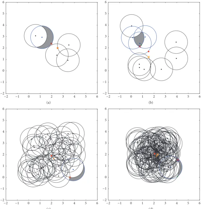
The pseudocode of the ABC is given as Algorithm 2.
3.2. Crossover-Based Artificial Bee Colony Algorithm for
Solving the CWP. Recent improved variant of the ABC for
COPs, called crossover-based artificial bee colony, is also used to solve the constrained Weber problem [54]. The main modifications introduced in the CB-ABC are related to the search operators used in each bee phase in order to improve the distribution of good information between solutions [54]. The differences between the CB-ABC and the ABC for COPs are given as follows.
In the employed bee phase, the CB-ABC algorithm uses modified search equation (5), in which𝜑is the same random number of each parameter𝑗which will be changed. Also, the CB-ABC does not use the fixed value of MR control parame-ter. Value of MR linearly increases from0.1to the predefined
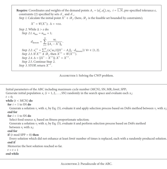
Require: Coordinates and weights of the demand points𝐴𝑖= (𝑎𝑖1, 𝑎2𝑖), 𝑤𝑖, 𝑖 = 1, 𝑁, pre-specified tolerance𝜀, constraints (2) specified by setsS<andS>.
Step 1. Calculate the initial point𝑋∗∈R𝑓(here,R𝑓is the feasible set bounded by constraints); 𝑋∗=C(𝑋∗); Δ = +∞.
Step 2. WhileΔ > 𝜀do:
Step 2.1.𝑛iter= 𝑛iter+ 1; 𝑑denom= 𝑁 ∑ 𝑖=1 𝑤𝑖 ‖𝐴𝑖− 𝑋∗‖2. Step 2.2.𝑥∗∗𝑟 = ∑𝑁𝑖=1(𝑥∗𝑟𝑤𝑖/(‖𝑋∗− 𝐴𝑖‖2⋅ 𝑑denom)) ∀𝑟 ∈ {1, 2}. Step 2.3. If𝑋∗∗∉R𝑓then𝑋∗∗=C(𝑋∗∗). Step 2.4.Δ = ‖𝑋∗− 𝑋∗∗‖;𝑋∗= 𝑋∗∗.
Step 2.5. Continue Step2.
Step 3. STOP, return𝑋∗∗.
Algorithm 1: Solving the CWP problem.
Initial parameters of the ABC including maximum cycle number (MCN), SN,MR, 𝑙𝑖𝑚𝑖𝑡,SPP; Generate initial population𝑥𝑖(𝑖 = 1, 2, . . . ,SN) randomly in the search space and evaluate each𝑥𝑖;
𝑡 = 0;
while(𝑡 <MCN)do for𝑖 = 1to SNdo
Generate a solutionV𝑖with𝑥𝑖by Eq. (5), evaluate it and apply selection process based on Deb’s method betweenV𝑖with𝑥𝑖;
end for
for𝑖 = 1to SNdo
Select food source𝑥𝑙based on fitness proportionate selection;
Generate a solutionV𝑙with𝑥𝑙by Eq. (5), evaluate it and perform selection process based on Deb’s method
betweenV𝑙with𝑥𝑙;
end for
if(𝑡mod SPP= 0)then
Every solution which did not enhance at least𝑙𝑖𝑚𝑖𝑡number of times is replaced, each with a randomly produced solution.
end if
Memorize the best solution reached so far.
𝑡 = 𝑡 + 1 end while
Algorithm 2: Pseudocode of the ABC.
Table 1: The values of specific control parameters of the algorithms.
FA E-FA ABC CB-ABC
𝛼 0.25 𝛼 0.25 MR 0.8 MRmax 0.9 𝛽 1 𝛽 1.5 𝑙𝑖𝑚𝑖𝑡 SN 𝑙𝑖𝑚𝑖𝑡 1
𝛾 1 𝛾 1 SPP SN SPP 50
𝑃 0.3
value MRmaxin the first𝑃 ∗MCN iterations, while the value
MR = MRmaxis used in the remaining iterations. The value
of𝑃is defined in Table 1.
In the onlooker bee phase, the CB-ABC proposes a new search equation with the aim of enabling better exploration of the neighborhood of the high-quality solution. This equation is given by
V𝑖𝑗= 𝑥𝑖𝑗+ 𝜑 ⋅ (𝑥𝑙𝑗− 𝑥𝑘𝑗) , (6)
where𝜑is a uniform random number in range[−1, 1],𝑥𝑙and
𝑥𝑘represent the other two solutions selected randomly from
the population,𝑅𝑗 is a randomly chosen real number in the range[0, 1), and𝑗 = 1, 2.
In the scout bee phase, the CB-ABC uses uniform crossover operator to generate new solutions in a promising region of the search space. Therefore, after each SPPth iter-ation, each solution𝑥𝑖which did not improve𝑙𝑖𝑚𝑖𝑡number of times is replaced with a new solution which is created by
V𝑖𝑗={{ {
𝑦𝑗, if𝑅𝑗< 0.5
𝑥𝑖𝑗, otherwise, (7) where𝑦𝑗is the𝑗th element of the global best solution found so far,𝑅𝑗is a randomly chosen real number in range[0, 1), and𝑗 = 1, 2.
Initial parameters of the FA including SN,MCN, 𝛼0, 𝛽0, 𝛾.
Generate initial population of fireflies𝑥𝑖(𝑖 = 1, 2, . . . ,SN) randomly distributed in the solution space. Assume that𝜑(𝑥𝑖)is the expanded objective function of𝑥𝑖(𝑖 = 1, 2, . . . ,SN) calculated by (10).
𝑡 = 0.
while𝑡 <MCNdo for𝑖 = 1to SNdo for𝑗 = 1to SNdo
if(𝜑(𝑥𝑗) < 𝜑(𝑥𝑖))then
Generate a new𝑥𝑖according to Eq. (8) and evaluate it.
end if end for end for 𝑡 = 𝑡 + 1. 𝛼(𝑡) = 𝛼(𝑡 − 1) ⋅ (10.0−4.0/0.91/MCN ).
Rank the fireflies and memorize the best solution achieved so far.
end while
Algorithm 3: Pseudocode of the FA.
3.3. Firefly Algorithm for Solving the CWP. In order to solve
the CWP we have employed a numerical optimization version of the FA for COPs, introduced in [37]. In the FA, a colony of artificial fireflies searches for good solutions in every iteration.
The search operator represents the movement of a firefly
𝑖to another more attractive or brighter firefly𝑗and it is given by
𝑥𝑖𝑘= 𝑥𝑖𝑘+ 𝛽 ⋅ (𝑥𝑗𝑘− 𝑥𝑖𝑘) + 𝛼 ⋅ 𝑆𝑘⋅ (rand𝑘− 12), (8)
where the second term is due to the attraction and the third term is a randomization term.
In the second term of (8), the parameter 𝛽 is the attractiveness of fireflies which is calculated according to the following monotonically decreasing function [62]:
𝛽 = 𝛽0⋅ 𝑒−𝛾⋅𝑟 2
𝑖𝑗, (9)
where𝑟𝑖𝑗denotes the distance between firefly𝑥𝑖and firefly
𝑥𝑗, while𝛽0and𝛾are predetermined algorithm parameters:
maximum attractiveness value and absorption coefficient, respectively. Distance between fireflies is calculated by the Euclidean distance.
In the third term of (8),𝛼 ∈ [0, 1] is a randomization parameter, 𝑆𝑘 are the scaling parameters, and rand𝑘 is a random number uniformly distributed between0and1. The scaling parameters 𝑆𝑘 (𝑘 = 1, 2) are calculated by 𝑆𝑘 =
|𝑢𝑘− 𝑙𝑘|, where𝑙𝑘and𝑢𝑘 are the lower and upper bound of
the parameter 𝑥𝑖𝑘. Diversity of solutions is controlled by the randomization parameter𝛼which needs to be reduced gradually during iterations so that it can vary with the iter-ation counter𝑡[63].
In the FA for solving CWP, penalty functions approach is used in order to handle the constraints. In this way, a constrained problem is solved as an unconstrained one. A
general formula of calculation penalty functions is given in [64] by 𝜑 (𝑋) = 𝑓 (𝑋) +∑𝑞 𝑗=1𝑟𝑗⋅ max(0, 𝑔𝑗(𝑋))2+ 𝑚 ∑ 𝑗=𝑞+1𝑐𝑗 ⋅ ℎ𝑗(𝑋), (10)
where𝜑(𝑋)is the new (expanded) objective function to be optimized, 𝑟𝑗 and𝑐𝑗 are positive constants normally called “penalty factors,”𝑞is the number of inequality constraints, and𝑚 − 𝑞is the number of equality constraints for a given problem. We found it suitable to set each 𝑟𝑖 to the value
𝑟𝑖= 108. The penalty factors for equality constraints were not
used, since these problems have only inequality constraints. The pseudocode of the FA is given as Algorithm 3.
3.4. An Enhanced Firefly Algorithm for Solving the CWP. An
enhanced firefly algorithm for COPs is presented in [55] and it is also applied to solve the CWP. Two modifications are incorporated in the E-FA in order to improve the perfor-mance of the firefly algorithm for COPs.
The first modification is related to using Deb’s rules instead of the penalty approach. Three feasibility rules are employed instead of the greedy selection in order to decide which firefly is brighter. These rules are also used each time after (8) is applied in order to decide whether the solution will be updated. Evaluation of solution population is given as Algorithm 4.
The second modification is employing the geometric progression reduction scheme to reduce the scaling factors
𝑆𝑘at the end of each cycle, by the rule
𝑆𝑘(𝑡) = 𝑆𝑘(𝑡 − 1) ⋅ 𝜃1/MCN, (11)
where MCN is the maximum cycle number,𝑡is the current iteration number, and𝜃 = 10.0−4.0/0.9.
for𝑖 = 1to SNdo for𝑗 = 1to SNdo
if(𝑥𝑗is better than𝑥𝑖based on Deb’s rules)then for𝑘 = 1to𝐷(dimension of the problem)do
𝑔𝑘= 𝑥𝑖𝑘+ 𝛽 ⋅ (𝑥𝑗𝑘− 𝑥𝑖𝑘) + 𝛼 ⋅ 𝑆𝑘⋅ (rand𝑘− 1/2) end for
if(𝑔is better than𝑥𝑖based on Deb’s rules)then 𝑥𝑖= 𝑔 {the solution is updated}
end if end if end for end for
Algorithm 4: Evaluation of a new population in the E-FA.
4. Experimental Study
The ABC, CB-ABC, FA, and E-FA are implemented in the Java programming language on a PC Intel Core i5-3300@3 GHz with 4 GB of RAM. The heuristic algorithm based on the modified Weiszfeld procedure is also implemented for the purpose of comparison with the metaheuristic approaches.
4.1. Benchmark Functions. The performance of the four
meta-heuristics techniques and behavior of the heuristic algorithm are evaluated through eighteen test instances of the single-facility constrained Weber problems with the connected feasible region bounded by arcs with equal radius.
The benchmark problems with the increasing number of input points are randomly generated according to the algo-rithm given in [44]. These problems have 5, 10, 50, 100, 250, and 500 input points. Three different random test problems are generated for each number of input points. Hence, these test instances have a nonconvex feasible set given from 5 up to 500 constraints.
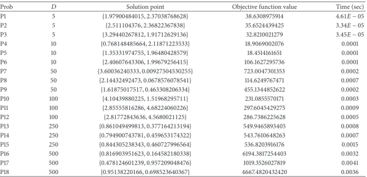
Four example problems, named P1, P4, P7, and P10 with 5, 10, 50, and 100 input points, respectively, are shown in Figure 1. In each test image, the feasible region is represented by a gray surface area and the final solution obtained by the heuristic algorithm [44] is represented by a red cross.
4.2. Parameter Settings. The solution number (SN) in the four
metaheuristic algorithms was set to 20. The maximum number of fitness function evaluations (FEs) was used as the stopping criterion. The allowed FEs were set to8000. In addi-tion, the metaheuristic algorithms presented in Section 2 have several other control parameters that considerably influence their performance. The values of these control parameters are presented in Table 1.
In order to calculate FEs researchers usually use the rule SN∗MCN, where MCN is the maximum number of iterations [65, 66]. Hence, the FA and E-FA were terminated after400 iterations. The number of consumed fitness evaluations in each iteration of the ABC and CB-ABC algorithms is 2 ∗ SN, since it calculates the solutions both in the employed bee and in onlooker bee phase [65]. Therefore, to ensure
a fair comparison, the ABC and CB-ABC algorithms were terminated after200iterations.
For the FA, it is widely reported in the literature that the light absorption coefficient𝛾 = 𝑂(1), the initial attractiveness
𝛽0 = 1, and the initial randomness factor𝛼0 ∈ [0, 1]can be
used for most applications [36, 62]. It can be seen from Table 1 that the value of the parameter𝛾was set to1and the initial value of𝛼was set to0.25for both FA and E-FA. A typical value of𝛽0= 1is used in the FA. It was empirically determined that slightly higher value of the parameter𝛽0is more suitable for the E-FA. Hence𝛽0= 1.5was adapted. For the ABC and CB-ABC algorithms, the values of the specific control parameters were taken from [53, 54], where these algorithms were proposed to solve COPs. Especially for the CB-ABC, it was empirically determined that a lower value of the scout pro-duction period SPP is more appropriate for solving the CWP. Therefore, it was set to 50. Each of the experiments was repeated for30runs.
4.3. Analysis of Solution Quality and Robustness. The
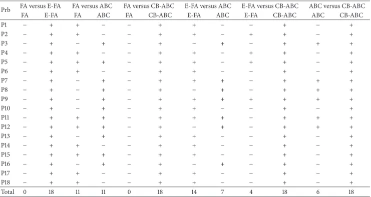
coordi-nates of the solution, corresponding objective function value, and the CPU time (in seconds) obtained by the heuristic algo-rithm are arranged in Table 2. To analyze the solution quality of the tested four metaheuristic algorithms, the best values, mean values, and standard deviations have been obtained by the ABC, CB-ABC, FA, and E-FA algorithms over30runs. Significance tests are used to achieve reliable comparisons. According to [67], two-sample 95%-confidence t-test was conducted between each pair of compared metaheuristics on every benchmark function. The calculated best results are presented in Table 3, while the mean values and standard deviations are arranged in Table 4. Results of two-samplet -tests are reported in Table 5. The sign “+” indicates that the associated comparative algorithm is significantly better than the other one, while the sign “−” indicates it is significantly worse than the opposite one. If both algorithms show similar performance, they are both marked by “+.”
Kazakovtsev in [44] experimentally proved the conver-gence of the heuristic algorithm on randomly generated test problems. Hence, the calculated best values of the meta-heuristics can be compared to the results found by the heuris-tic approach in order to show the ability of the metaheurisheuris-tic algorithm to reach the near-optimal result. The obtained mean and standard deviation values indicate the robustness of the metaheuristic approaches.
It can be seen from Table 3 that each of the metaheuristic algorithms found the best results which are very close to the results obtained by the heuristic algorithm. More precisely, the FA obtained 10 better best results (P2, P4, P5, P6, P8, P9, P11, P16, P17, and P18) and 8 worse best results with respect to the heuristic approach. The E-FA obtained 11 better best results (P1, P2, P4, P5, P6, P8, P9, P11, P16, P17, and P18), one equal best result (P3) and 6 slightly worse best results in comparison with the heuristic approach. The ABC algorithm achieved 12 better best results (P2, P4, P5, P6, P8, P9, P10, P11, P12, P16, P17, and P18), one equal best result (P3), and 5 worse best results with respect to the heuristic approach. The algorithm CB-ABC was able to find better or the same best solution for all problems with respect to the heuristic
6 5 4 3 2 1 0 −1 −2 −2 −1 0 1 2 3 4 5 6 (a) 6 5 4 3 2 1 0 −1 −2 −2 −1 0 1 2 3 4 5 6 (b) 6 5 4 3 2 1 0 −1 −2 −2 −1 0 1 2 3 4 5 6 (c) 6 5 4 3 2 1 0 −1 −2 −2 −1 0 1 2 3 4 5 6 (d)
Figure 1: Example problems with (a) 5 points (P1), (b) 10 points (P4), (c) 50 points (P7), and (d) 100 points (P10).
algorithm, with the exception of the problem P7, where the CB-ABC obtained slightly worse best result.
In terms of best results from Table 3, it can be noticed that the CB-ABC achieved better and in several cases the same values in comparison with each considered metaheuristic approach. Further, each of the improved metaheuristics, the E-FA and CB-ABC, obtained better best results with respect to both original metaheuristic algorithms for the majority of test problems. If we compare the performance of the original ABC to that of the original FA, it can be seen that both algorithms show similar ability to reach the near-optimal result; that is, the ABC has found 9 slightly better best results and 9 slightly worse ones compared to the FA.
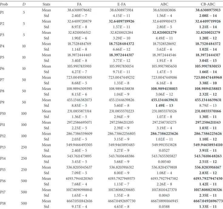
From Table 4, it can be seen that mean and standard deviation results obtained by the CB-ABC are much better than the results obtained by the other metaheuristic algo-rithms. The CB-ABC converged consistently to the same solution with the same objective function value and very lower standard deviation. If we compare the robustness of the remaining three metaheuristics, it can be noticed that the E-FA outperformed the FA and ABC. Compared with the ABC, the FA obtained9 better mean results and standard deviation values (P1, P2, P4, P6, P11, P13, P14, P17, and P18). The remaining mean and standard deviation results are better in the case of the ABC algorithm, with the exception of P5 and P15 where the FA and ABC show similar performances.
Table 2: The solution point, corresponding objective function, and time in seconds provided by the heuristic algorithm.
Prob 𝐷 Solution point Objective function value Time (sec)
P1 5 {1.97900484015, 2.37038768628} 38.6308975914 4.61𝐸 − 05 P2 5 {2.511104376, 2.36822367838} 35.6524439425 3.34𝐸 − 05 P3 5 {3.29440267812, 1.91712629136} 32.8210021279 3.45𝐸 − 05 P4 10 {0.768148485664, 2.11871223533} 18.9069002076 0.0001 P5 10 {1.35331974755, 1.96480428579} 18.4514161651 0.0001 P6 10 {2.40607643306, 1.99679256415} 106.1627295736 0.0001 P7 50 {3.60036240333, 0.00927504530255} 723.0047301353 0.0002 P8 50 {2.14432492473, 0.0678576078541} 114.6249767471 0.0007 P9 50 {1.61875017517, 0.463308206334} 455.1344852622 0.0002 P10 100 {4.10439880225, 1.51968295711} 231.0855570171 0.0003 P11 100 {2.85555816286, 4.68224060226} 297.6045429275 0.0009 P12 100 {2.81772843636, 4.5680021125} 286.7386225628 0.0005 P13 250 {0.861049499813, 0.377164213194} 549.9465893405 0.0008 P14 250 {0.794900743781, 0.459653174322} 543.7610648263 0.0007 P15 250 {0.844305238343, 0.460727996564} 536.8203916176 0.0015 P16 500 {0.816903951623, 0.164582180338} 6194.3817254403 0.0032 P17 500 {0.478124601239, 0.957209048476} 1019.3526027819 0.0041 P18 500 {0.95138220166, 0.698523640367} 4667.4820432420 0.0036
Table 3: Comparison of the best solutions obtained from the FA, E-FA, ABC, and CB-ABC algorithms for 18 test instances over 30 runs.
Prob 𝐷 FA E-FA ABC CB-ABC
P1 5 38.6308975997 38.6308975913 38.6309142364 38.6308975913 P2 5 32.6409719983 32.6409719926 32.6409728972 32.6409719926 P3 5 32.8210027975 32.8210021279 32.8210021279 32.8210021279 P4 10 18.7528484406 18.7528484372 18.7528484934 18.7528484372 P5 10 18.3972444320 18.3972444317 18.3972444324 18.3972444317 P6 10 105.9917830548 105.9917830153 105.9917835005 105.9917830153 P7 50 723.0047799356 723.0047449044 723.0047448967 723.0047448967 P8 50 108.9894160829 108.9894138822 108.9894138815 108.9894138815 P9 50 455.1344837962 455.1344639665 455.1344639631 455.1344639631 P10 100 231.0855604428 231.0855570172 231.0855570166 231.0855570165 P11 100 297.2586347001 297.2586211173 297.2586217396 297.2586211143 P12 100 286.7386294462 286.7386225632 286.7386225626 286.7386225626 P13 250 549.9466005355 549.9465893424 549.9476076576 549.9465893411 P14 250 543.7610916668 543.7610648272 543.7611199289 543.7610648263 P15 250 536.8204201801 536.8203916186 536.8203922596 536.8203916167 P16 500 6193.7933019446 6193.7927947779 6193.7927947450 6193.7927947450 P17 500 1017.8088547714 1017.8088230476 1017.8091304405 1017.8088230326 P18 500 4667.0497043757 4667.0492697127 4667.0515567517 4667.0492696773
Results of two-samplet-tests are given in Table 5, and they show that the CB-ABC is significantly better than the FA, E-FA, and ABC on18,14, and12test problems, respectively. It is similar to the FA, E-FA, and ABC on0,4, and6problems, respectively. It is worth noting that the FA, E-FA, and ABC can not outperform the CB-ABC on any problem. Further, it can be observed that the E-FA is significantly better than the FA on each test problem. In comparison with the ABC, the E-FA is superior on11test problems, inferior on 4 problems,
and similar on3benchmarks. When comparing the perfor-mances of the FA and ABC it can be noticed that the FA is significantly better than the ABC on7problems, while it is inferior to it on7problems. The FA and ABC show similar performances on4benchmarks.
According to the results reported in Tables 3, 4, and 5, we can conclude that the CB-ABC and E-FA exhibit superior performances compared to both original versions, ABC and FA, in solving constrained Weber problems with
Table 4: Comparison of the mean values and standard deviations obtained from the FA, E-FA, ABC, and CB-ABC algorithms for 18 test instances over 30 runs.
Prob 𝐷 Stats FA E-FA ABC CB-ABC
P1 5 Mean 38.6308978682 38.6308975914 38.6310183806 38.6308975913 Std 2.40𝐸 − 7 4.15𝐸 − 11 1.56𝐸 − 4 2.08E−14 P2 5 Mean 32.6409720879 32.6409719926 32.6409910473 32.6409719926 Std 8.97𝐸 − 8 1.57𝐸 − 11 2.80𝐸 − 5 1.21E−14 P3 5 Mean 32.8210056512 32.8210021284 32.8210021279 32.8210021279 Std 1.90𝐸 − 6 3.29𝐸 − 10 4.49𝐸 − 11 1.20E−12 P4 10 Mean 18.7528484769 18.7528484372 18.7528528692 18.7528484372 Std 1.14𝐸 − 8 6.66𝐸 − 12 5.62𝐸 − 6 1.02E−14 P5 10 Mean 18.3972444465 18.3972444317 18.3972444546 18.3972444317 Std 3.40𝐸 − 8 3.77𝐸 − 12 1.91𝐸 − 8 3.04E−15 P6 10 Mean 105.9917835910 105.9917830154 105.9917985650 105.9917830153 Std 4.27𝐸 − 7 9.71𝐸 − 11 1.47𝐸 − 5 1.66E−14 P7 50 Mean 723.0049108305 723.0047449232 723.0047449186 723.0047448968 Std 8.68𝐸 − 5 1.33𝐸 − 8 6.16𝐸 − 8 3.38E−10 P8 50 Mean 108.9894309395 108.9894138838 108.9894138815 108.9894138815 Std 8.15𝐸 − 6 1.04𝐸 − 9 3.06𝐸 − 12 2.32E−12 P9 50 Mean 455.1346382073 455.1344639826 455.1344639631 455.1344639631 Std 8.83𝐸 − 5 5.60𝐸 − 8 1.49E−13 8.79𝐸 − 13 P10 100 Mean 231.0855873314 231.0855570223 231.0855570526 231.0855570166 Std 1.36𝐸 − 5 2.94𝐸 − 9 1.07𝐸 − 8 1.30E−11 P11 100 Mean 297.2586695071 297.2586211205 297.2587315275 297.2586211143 Std 2.23𝐸 − 5 2.39𝐸 − 9 3.19𝐸 − 4 1.03E−11 P12 100 Mean 286.7386559609 286.73862256805 286.7386225626 286.7386225626 Std 2.03𝐸 − 5 3.15𝐸 − 9 1.02𝐸 − 11 1.10E−12 P13 250 Mean 549.9466493305 549.9465893483 549.9913513828 549.94658934110 Std 2.40𝐸 − 5 3.27𝐸 − 9 0.0527 3.91E−11 P14 250 Mean 543.7611473895 543.7610648386 543.7655305827 543.7610648263 Std 3.45𝐸 − 5 5.68𝐸 − 9 0.00540 2.51E−12 P15 250 Mean 536.8205045637 536.8203916312 536.8204579818 536.8203916167 Std 7.09𝐸 − 5 8.00𝐸 − 9 1.08𝐸 − 4 2.83E−12 P16 500 Mean 6193.7944120365 6193.7927949375 6193.7927947582 6193.7927947450 Std 7.68𝐸 − 4 1.13𝐸 − 7 2.26𝐸 − 8 1.42E−11 P17 500 Mean 1017.8090988841 1017.8088230685 1017.8110427370 1017.8088230326 Std 1.63𝐸 − 4 1.55𝐸 − 8 0.0043 2.35E−11 P18 500 Mean 4667.0511842616 4667.0492697730 4667.0890166945 4667.0492696773 Std 9.17𝐸 − 4 4.63𝐸 − 8 0.0588 1.33E−11
the connected feasible region bounded by arcs. Further, from these results and according to the results from Table 2, it is clear that the CB-ABC outperformed all other three meta-heuristic algorithms as well as the meta-heuristic algorithm with respect to the quality of the obtained results. Although the CB-ABC has more accurate and more stable results than the remaining three metaheuristics, all four metaheuristic approaches perform better than or equal to the heuristic approach with respect to the quality of the obtained results for most of the tested problems.
4.4. Computational Time Analysis. In order to compare the
computational cost of the four metaheuristic algorithms, we computed the mean of the CPU times over30runs taken by
each metaheuristic algorithm. These results are reported in Table 6. The results from Table 6 show that the execution time for each of the metaheuristics approaches linearly increases when the number of the constraints or input points increases. By comparing computational times for the ABC and CB-ABC algorithms with respect to the FA and E-FA, it is observable that ABC and CB-ABC algorithms are about 4 times faster than the FA and about20times faster than the E-FA for the majority of test problems. The computational times of the ABC and CB-ABC algorithms are not significantly different. In addition, when the number of constraints is
500 that time is less than 0.1seconds. The computational time requirements for the E-FA algorithm are about five times greater compared to the FA and when the number
Table 5: The results of 95%-confidence two-sample𝑡-test over each test problem.
Prb FA versus E-FA FA versus ABC FA versus CB-ABC E-FA versus ABC E-FA versus CB-ABC ABC versus CB-ABC FA E-FA FA ABC FA CB-ABC E-FA ABC E-FA CB-ABC ABC CB-ABC
P1 − + + − − + + − − + − + P2 − + + − − + + − + + − + P3 − + − + − + − + − + + + P4 − + + − − + + − + + − + P5 − + + + − + + − + + − + P6 − + + − − + + − − + − + P7 − + − + − + + + − + + + P8 − + − + − + − + − + + + P9 − + − + − + + + + + + + P10 − + − + − + + − − + − + P11 − + + + − + + + − + + + P12 − + + + − + − + − + + + P13 − + − + − + + − − + − + P14 − + + − − + + − − + − + P15 − + + + − + + − − + − + P16 − + − + − + − + − + − + P17 − + + − − + + − − + − + P18 − + + − − + + − − + − + Total 0 18 11 11 0 18 14 7 4 18 6 18
Table 6: Mean of the CPU times (in seconds) obtained from the FA, E-FA, ABC, and CB-ABC algorithms for 18 test instances over 30 runs.
Prob 𝐷 FA E-FA ABC CB-ABC
P1 5 0.022 0.036 0.004 0.004 P2 5 0.020 0.044 0.005 0.004 P3 5 0.022 0.040 0.004 0.004 P4 10 0.025 0.060 0.005 0.006 P5 10 0.022 0.060 0.006 0.006 P6 10 0.025 0.062 0.004 0.005 P7 50 0.056 0.226 0.013 0.016 P8 50 0.052 0.224 0.014 0.014 P9 50 0.057 0.252 0.014 0.010 P10 100 0.090 0.690 0.035 0.043 P11 100 0.090 0.738 0.034 0.043 P12 100 0.086 0.544 0.022 0.025 P13 250 0.200 0.990 0.044 0.044 P14 250 0.216 1.316 0.048 0.051 P15 250 0.194 1.046 0.045 0.042 P16 500 0.376 2.182 0.082 0.093 P17 500 0.360 1.990 0.080 0.091 P18 500 0.374 2.128 0.081 0.094
of constraints or input points is 500 that time is about two seconds.
Compared with the computational time results of the heuristic approach, which are presented in Table 2, it can be seen that the heuristic algorithm requires less computational time than the four metaheuristic algorithms. However, the computational time of the four metaheuristics is reasonable
and it can be considered as negligible, since it is less than one second in most cases.
5. Conclusion
The constrained Weber problem with feasible region bound-ed by arcs represents a problem of a nonconvex optimization.
Finding a global optimum of such a problem is difficult considering the fact that it has multiple locally optimal points within the feasible region. Metaheuristic approaches for solving this problem are suitable choice, since these tech-niques can obtain quality results in a reasonable amount of time.
The performances of two prominent swarm-intelligence algorithms (the artificial bee colony and firefly algorithm) and their recently proposed improved versions for constrained optimization (the crossover-based artificial bee colony and enhanced firefly algorithm) are compared. The heuristic algorithm based on modified Weiszfeld procedure is also implemented for the purpose of the comparison with the metaheuristic approaches.
The four metaheuristic algorithms are compared on eigh-teen randomly generated test instances in which the number of input points or constraints increases up to 500. Numerical results indicate that all four metaheuristic algorithms are superior compared to the heuristic approach with respect to the precision of the results, with the notable ascendancy of the CB-ABC algorithm. In terms of the execution time, the ABC and CB-ABC are more efficient than the FA and E-FA. Although these four algorithms require somewhat higher computational cost than the heuristic approach, the CPU times for all these algorithms are reasonable and grow at a linear rate as the number of input points or constraints increases. Finally, it turns out that the CB-ABC algorithm is superior compared to other metaheuristics with respect to the quality of the results, robustness, and computational efficiency.
From this research it can be concluded that metaheuristic approaches can be successfully used for problems with max-imum and minmax-imum distance limits. Further, this research encourages the application of the metaheuristic algorithms for solving some other complex constrained optimization problems of practical importance.
Conflicts of Interest
The authors declare that there are no conflicts of interest regarding the publication of this paper.
Acknowledgments
The second and third authors gratefully acknowledge support from the Project supported by Ministry of Education and Sci-ence of Republic of Serbia, Grant no. 174013. The first, third, and fifth authors gratefully acknowledge support from the Project Applying Direct Methods for Digital Image Restoring of the Goce Delˇcev University. The fourth author gratefully acknowledges support from the Ministry of Education and Science of Russian Federation (Project 2.5527.2017/8.9).
References
[1] R. Z. Farahani and M. Hekmatfar,Facility Location: Concepts, Models, Algorithms and Case Studies, Springer-Verlag, Berlin, Germany, 2009.
[2] A. Weber,Ueber den Standort der Industrien, Erster Teil: Reine Theorie des Standortes, J.C.B. Mohr, T¨ubingen, Germany, 1909. [3] G. Wesolowsky, “The Weber problem: history and perspectives,”
Location Science, vol. 1, pp. 5–23, 1993.
[4] Z. Drezner, K. Klamroth, A. Sch¨obel, and G. O. Wesolowsky, “The Weber problem,” inFacility Location, pp. 1–36, Springer, Berlin, Germany, 2002.
[5] P. S. Stanimirovi´c, M. S. ´Ciri´c, L. A. Kazakovtsev, and I. A. Osinuga, “Single-facility Weber location problem based on the lift metric,” Facta Universitatis. Series: Mathematics and Informatics, vol. 27, no. 2, pp. 175–190, 2012.
[6] R. F. Love, W. G. Truscott, and J. Walker, “Facilities Location: Models and Methods,”International Journal of Machine Learn-ing and Cybernetics, North-Holland, New York, 1988.
[7] E. Weiszfeld, “Sur le point sur lequel la somme des distances de n points donnes est minimum,”Tohoku Mathematical Journal, vol. 43, no. 1, pp. 335–386, 1937.
[8] Y. Vardi and C.-H. Zhang, “A modified Weiszfeld algorithm for the Fermat-WEBer location problem,”Mathematical Program-ming, vol. 90, no. 3, Ser. A, pp. 559–566, 2001.
[9] C. Szegedy,Some Applications of the Combinatorial Laplacian, University of Bonn, 2005.
[10] P. Hansen, N. Mladenovi´c, and E. Taillard, “Heuristic solution of the multisource Weber problem as a𝑝-median problem,”
Operations Research Letters, vol. 22, no. 2-3, pp. 55–62, 1998. [11] S. Gonzalez-Martin, A. Ferrer, A. A. Juan, and D. Riera,
“Solving non-smooth arc routing problems throughout biased-randomized heuristics,” Advances in Intelligent Systems and Computing, vol. 262, pp. 451–462, 2014.
[12] A. H. Gandomi, X.-S. Yang, S. Talatahari, and A. H. Alavi, “Metaheuristic algorithms in modeling and optimization,” in
Metaheuristic Applications in Structures and Infrastructures, A. H. Gandomi, X.-S. Yang, S. Talatahari, and A. H. Alavi, Eds., pp. 1–24, Elsevier, 2013.
[13] R. Mart´ı and G. Reinelt,The Linear Ordering Problem: Exact and Heuristic Methods in Combinatorial Optimization, vol. 175, Springer, New York, NY, USA, 2011.
[14] A. Afshar, F. Massoumi, A. Afshar, and M. A. Mari˜no, “State of the art review of ant colony optimization applications in water resource management,”Water Resources Management, vol. 29, no. 11, pp. 3891–3904, 2015.
[15] A. Banks, J. Vincent, and C. Anyakoha, “A review of particle swarm optimization. I. Background and development,”Natural Computing. An International Journal, vol. 6, no. 4, pp. 467–484, 2007.
[16] I. Fister Jr., M. Perc, S. M. Kamal, and I. Fister, “A review of chaos-based firefly algorithms: perspectives and research challenges,”Applied Mathematics and Computation, vol. 252, pp. 155–165, 2015.
[17] I. Fister, X. S. Yang, and D. Fister, “Cuckoo search: a brief literature review,” in Cuckoo Search and Firefly Algorithm: Theory and Applications, Xin-She Yang, Ed., pp. 49–62, Springer International Publishing.
[18] I. Fister, I. Fister Jr., X.-S. Yang, and J. Brest, “A comprehensive review of firefly algorithms,”Swarm and Evolutionary Compu-tation, vol. 13, no. 1, pp. 34–46, 2013.
[19] D. Karaboga, B. Gorkemli, C. Ozturk, and N. Karaboga, “A comprehensive survey: artificial bee colony (ABC) algorithm and applications,”Artificial Intelligence Review, vol. 42, pp. 21– 57, 2014.
[20] M. Bilal, M. Shams-ur-Rehman, and M. A. Jaffar, “Reconstruc-tion: Image restoration for space variant degradation,”Smart Computing Review, vol. 3, no. 4, pp. 220–232, 2013.
[21] P. Siarry,Optimisation in Signal and Image Processing, Wiley-ISTE, 2009.
[22] X. Yang, S. F. Chien, and T. O. Ting, “Computational Intelligence and Metaheuristic Algorithms with Applications,”The Scientific World Journal, vol. 2014, Article ID 425853, 4 pages, 2014. [23] I. Fister Jr., X.-S. Yang, I. Fister, J. Brest, and D. Fister, “A
brief review of nature-inspired algorithms for optimization,”
Elektrotehniˇski Vestnik, vol. 80, no. 3, pp. 1–7, 2013.
[24] M. Dorigo, V. Maniezzo, and A. Colorni, “Ant system: optimiza-tion by a colony of cooperating agents,”IEEE Transactions on Systems, Man, and Cybernetics B: Cybernetics, vol. 26, no. 1, pp. 29–41, 1996.
[25] B. C. Mohan and R. Baskaran, “A survey: ant colony opti-mization based recent research and implementation on several engineering domain,”Expert Systems with Applications, vol. 39, no. 4, pp. 4618–4627, 2012.
[26] R. F. Tavares Neto and M. Godinho Filho, “Literature review regarding ant colony optimization applied to scheduling prob-lems: guidelines for implementation and directions for future research,”Engineering Applications of Artificial Intelligence, vol. 26, no. 1, pp. 150–161, 2013.
[27] J. Kennedy and R. Eberhart, “Particle swarm optimization,” inProceedings of the IEEE International Conference on Neural Networks (ICNN ’95), vol. 4, pp. 1942–1948, Perth, Western Australia, November-December 1995.
[28] A. Banks, J. Vincent, and C. Anyakoha, “A review of particle swarm optimization. II. Hybridisation, combinatorial, multicri-teria and constrained optimization, and indicative applications,”
Natural Computing. An International Journal, vol. 7, no. 1, pp. 109–124, 2008.
[29] A. Khare and S. Rangnekar, “A review of particle swarm optimization and its applications in Solar Photovoltaic system,”
Journal Applied Soft Computing, vol. 13, no. 5, pp. 2997–3006, 2013.
[30] B. Akay and D. Karaboga, “A modified artificial bee colony algo-rithm for real-parameter optimization,”Information Sciences, vol. 192, pp. 120–142, 2012.
[31] D. Karaboga, “An Idea Based on Honey Bee Swarm for Numer-ical Optimization,” TechnNumer-ical Report-TR06, Erciyes University, Engineering Faculty, Computer Engineering Department, 2005. [32] A. Baykasoglu, L. Ozbakir, and P. Tapkan, “Artificial bee colony algorithm and its application to generalized assignment prob-lem,” inSwarm Intelligence, Focus on Ant and Particle Swarm Optimization, F. T. S. Chan and M. K. Tiwari, Eds., pp. 113–144, I-Tech Education and Publishing, Vienna, Austria, 2007. [33] S. Zhang and S. Liu, “A novel artificial bee colony algorithm for
function optimization,”Mathematical Problems in Engineering, vol. 2015, Article ID 129271, 10 pages, 2015.
[34] Y. Liang, Z. Wan, and D. Fang, “An improved artificial bee colony algorithm for solving constrained optimization prob-lems,”International Journal of Machine Learning and Cybernet-ics, vol. 8, no. 3, pp. 739–754, 2017.
[35] T. K. Sharma and M. Pant, “Shuffled Artificial Bee Colony Algorithm,”Soft Computing, pp. 1–20, 2016.
[36] X.-S. Yang, “Firefly algorithms for multimodal optimization,” in
Stochastic Algorithms: Foundations and Applications, vol. 5792 of
Lecture Notes in Computer Science, pp. 169–178, Springer, Berlin, 2009.
[37] A. H. Gandomi, X.-S. Yang, and A. H. Alavi, “Mixed variable structural optimization using firefly algorithm,”Computers and Structures, vol. 89, no. 23-24, pp. 2325–2336, 2011.
[38] M. Huang, J. Yuan, and J. Xiao, “An adapted firefly algorithm for product development project scheduling with fuzzy activity duration,” Mathematical Problems in Engineering, vol. 2015, Article ID 973291, 11 pages, 2015.
[39] X.-S. Yang and S. Deb, “Cuckoo search via L´evy flights,” in
Proceedings of the World Congress on Nature and Biologically Inspired Computing (NABIC ’09), pp. 210–214, Coimbatore, India, December 2009.
[40] Y. Lin, C. Zhang, and Z. Liang, “Cuckoo search algorithm with hybrid factor using dimensional distance,”Mathematical Problems in Engineering, vol. 2016, Article ID 4839763, 11 pages, 2016.
[41] A. R. Yildiz, “Cuckoo search algorithm for the selection of opti-mal machining parameters in milling operations,”International Journal of Advanced Manufacturing Technology, vol. 64, no. 1–4, pp. 55–61, 2013.
[42] M. Hakan Aky¨uz, T. ¨Oncan, and I. Kuban Altinel, “Beam search heuristics for the single and multi-commodity capaci-tated multi-facility weber problems,”Computers and Operations Research, vol. 40, no. 12, pp. 3056–3068, 2013.
[43] J.-L. Jiang and X.-M. Yuan, “A heuristic algorithm for con-strained multi-source Weber problem—the variational inequal-ity approach,”European Journal of Operational Research, vol. 187, no. 2, pp. 357–370, 2008.
[44] L. A. Kazakovtsev, “Algorithm for constrained Weber problem with feasible region bounded by arcs,”Facta Universitatis. Series: Mathematics and Informatics, vol. 28, no. 3, pp. 271–284, 2013. [45] M. Luis, S. Salhi, and G. Nagy, “Region-rejection based
heuris-tics for the capacitated multi-source Weber problem,” Comput-ers and Operations Research, vol. 36, no. 6, pp. 2007–2017, 2009. [46] S. M. H. Manzour-Al-Ajdad, S. A. Torabi, and K. Eshghi, “Single-source capacitated multi-facility weber problem—an iterative two phase heuristic algorithm,”Computers and Oper-ations Research, vol. 39, no. 7, pp. 1465–1476, 2012.
[47] M. Bischoff and K. Klamroth, “An efficient solution method for Weber problems with barriers based on genetic algorithms,”
European Journal of Operational Research, vol. 177, no. 1, pp. 22– 41, 2007.
[48] A. Ghaderi, M. S. Jabalameli, F. Barzinpour, and R. Rahmaniani, “An efficient hybrid particle swarm optimization algorithm for solving the uncapacitated continuous location-allocation problem,”Networks and Spatial Economics, vol. 12, no. 3, pp. 421–439, 2012.
[49] H. G. Gharravi and M. S. Farham, “Applying metaheuristic approaches on the single facility location problem with polygo-nal barriers,”International Journal of Metaheuristics, vol. 3, no. 4, p. 348, 2014.
[50] M. Saleh Farham, H. S¨ural, and C. Iyigun, “The Weber problem in congested regions with entry and exit points,”Computers and Operations Research, vol. 62, pp. 177–183, 2015.
[51] N. Javadian, R. Tavakkoli-Moghaddam, M. Amiri-Aref, and S. Shiripour, “Two meta-heuristics for a multi-period minisum location-relocation problem with line restriction,”International Journal of Advanced Manufacturing Technology, vol. 71, no. 5-8, pp. 1033–1048, 2014.
[52] N. Mohammadi, M. R. Malek, and A. A. Alesheikh, “A new GA based solution for capacitated multi source Weber problem,”
International Journal of Computational Intelligence Systems, vol. 3, no. 5, pp. 514–521, 2010.
[53] D. Karaboga and B. Akay, “A modified Artificial Bee Colony (ABC) algorithm for constrained optimization problems,” Ap-plied Soft Computing Journal, vol. 11, no. 3, pp. 3021–3031, 2011. [54] I. Brajevic, “Crossover-based artificial bee colony algorithm
for constrained optimization problems,”Neural Computing and Applications, vol. 26, no. 7, pp. 1587–1601, 2015.
[55] I. Brajevic and J. Ignjatovi´c, “An enhanced firefly algorithm for mixed variable structural optimization problems,” Facta Universitatis. Series: Mathematics and Informatics, vol. 30, no. 4, pp. 401–418, 2015.
[56] L. A. Kazakovtsev and P. S. Stanimirovic, “Algorithm for Weber problem with a metric based on the initial fare,”Journal of Applied Mathematics & Informatics, vol. 33, no. 1-2, pp. 157–172, 2015.
[57] Z. Drezner, C. Scott, and J.-S. Song, “The central warehouse location problem revisited,”IMA Journal of Management Math-ematics, vol. 14, no. 4, pp. 321–336 (2004), 2003.
[58] P. Hansen, D. Peeters, and J. F. Thisse, “Algorithm for a constrained weber problem,”Management Science, vol. 28, no. 11, pp. 1285–1295, 1982.
[59] P. Hansen, D. Peeters, and J.-F. Thisse, “Constrained Location and the Weber-Rawls Problem,”North-Holland Mathematics Studies, vol. 59, no. C, pp. 147–166, 1981.
[60] D. Karaboga and B. Basturk,Artificial Bee Colony (ABC) Opti-mization Algorithm for Solving Constrained OptiOpti-mization Prob-lems, Springer-Verlag, Berlin, Germany, LNAI 4529: IFSA’07, 2007.
[61] K. Deb, “An efficient constraint handling method for genetic algorithms,”Computer Methods in Applied Mechanics and Engi-neering, vol. 186, no. 2–4, pp. 311–338, 2000.
[62] X.-S. Yang,Nature-Inspired Metaheuristic Algorithms, Luniver Press, UK, 2010.
[63] X.-S. Yang, S. Deb, M. Loomes, and M. Karamanoglu, “A frame-work for self-tuning optimization algorithm,”Neural Comput-ing and Applications, vol. 23, no. 7-8, pp. 2051–2057, 2013. [64] E. Mezura-Montes and C. A. Coello Coello,
“Constraint-handling in nature-inspired numerical optimization: past, present and future,”Swarm and Evolutionary Computation, vol. 1, no. 4, pp. 173–194, 2011.
[65] M. Mernik, S.-H. Liu, D. Karaboga, and M. Crepinˇsek, “On clarifying misconceptions when comparing variants of the arti-ficial bee colony algorithm by offering a new implementation,”
Information Sciences, vol. 291, pp. 115–127, 2015.
[66] I. Fister, X. Yang, J. Brest, and I. Fister Jr., “Modified firefly algorithm using quaternion representation,” Expert Systems with Applications, vol. 40, no. 18, pp. 7220–7230, 2013. [67] E. Mezura-Montes and O. Cetina-Dom´ınguez, “Empirical
anal-ysis of a modified artificial bee colony for constrained numerical optimization,”Applied Mathematics and Computation, vol. 218, no. 22, pp. 10943–10973, 2012.