Machine learning methods for the analysis of liquid chromatography-mass spectrometry datasets in metabolomics

Doctoral Thesis

Machine Learning Methods for the

Analysis of Liquid

Chromatography-Mass Spectrometry

datasets in Metabolomics

Author:

Francesc Fern´andez Albert

Supervisors: Dr Alexandre Perera Lluna Dr Rafael Llorach Asunci´on

A thesis submitted in fulfilment of the requirements for the degree of Doctor in Biomedical Engineering

B2SLab

Department d’Enginyeria de Sistemes, Autom`atica i Inform`atica Industrial

Richard P. Feynman

Phfft! Facts! Facts are meaningless. You can use them to prove anything that is even remotely true.

Homer J. Simpson

”¡ ´Esto peta y repeta!”

Dr Rafael Llorach debugging the MAIT package

”El teorema del jard´ın? Es quan un es posa a explicar massa coses i acaba en un jard´ın, llavors... ´es igual, treu aquesta part.

Abstract

Departament d’Enginyeria de Sistemes, Autom`atica i Inform`atica Industrial

Doctor of Philosophy

Machine Learning Methods for the Analysis of Liquid Chromatography-Mass Spectrometry datasets in Metabolomics

by FrancescFern´andez Albert

Liquid Chromatography-Mass Spectrometry (LC/MS) instruments are widely used in Metabolomics. To analyse their output, it is necessary to use computational tools and algorithms to extract meaningful biological information. The main goal of this thesis is to provide with new computational methods and tools to process and analyse LC/MS datasets in a metabolomic context. A total of 4 tools and methods were developed in the context of this thesis.

First, it was developed a new method to correct possible non-linear drift effects in the retention time of the LC/MS data in Metabolomics, and it was coded as an R package called HCor. This method takes advantage of the retention time drift correlation found in typical LC/MS data, in which there are chromatographic regions in which their retention time drift is consistently different than other regions. Our method makes the hypothesis that this correlation structure is monotonous in the retention time and fits a non-linear model to remove the unwanted drift from the dataset. This method was found to perform especially well on datasets suffering from large drift effects when compared to other state-of-the art algorithms.

in which are corrected possible intensity drift effects by modelling the drift and then the data is normalised using the median of the resulting dataset. The drift was modelled using a Common Principal Components Analysis decomposition on the Quality Control classes and taking one, two or three Common Principal Components to model the drift space. This method was compared to four other drift correction and normalisation methods. The two-step method was shown to perform a better intensity drift removal than all the other methods. All the tested methods including the two-step method were coded as an R package called intCor and it is publicly available.

Third, a new processing step in the LC/MS data analysis workflow was proposed. In general, when LC/MS instruments are used in a metabolomic context, a metabolite may give a set of peaks as an output. However, the general approach is to consider each peak as a variable in the machine learning algorithms and statistical tests despite the important correlation structure found between those peaks coming from the same source metabolite. It was developed an strategy called peak aggregation techniques, that allow to extract a measure for each metabolite considering the intensity values of the peaks coming from this metabolite across the samples in study. If the peak aggregation techniques are applied on each metabolite, the result is a transformed dataset in which the variables are no longer the peaks but the metabolites. 4 different peak aggregation techniques were defined and, running a repeated random sub-sampling cross-validation stage, it was shown that the predictive power of the data was improved when the peak aggregation techniques were used regardless of the technique used.

Fourth, a computational tool to perform end-to-end analysis called MAIT was developed and coded under the R environment. The MAIT package is highly modular and pro-grammable which ease replacing existing modules for user-created modules and allow the users to perform their personalised LC/MS data analysis workflows. By default, MAIT takes the raw output files from an LC/MS instrument as an input and, by applying a set of functions, gives a metabolite identification table as a result. It also gives a set of figures and tables to allow for a detailed analysis of the metabolomic data. MAIT even accepts external peak data as an input. Therefore, the user can insert peak table obtained by any other available tool and MAIT can still perform all its other capabilities on this dataset like a classification or mining the Human Metabolome Dataset which is included in the package.

I know that this section might be the most read section of this document so I will try to thoroughly thank and acknowledge any individual (or set of) related to this work and I will also try not to disappoint anyone expecting some memorable words. It might seem a clich´e, but first of all I really would like to express my sincere gratitude to my advisors Dr Rafael Llorach (AKA Rafa) and Dr Alexandre Perera (AKA Alex). Both of them taught me so many things these years that would not fit in these pages, so I will just say that if I am far better scientist than four years ago, it is merely their merit. I especially thank Rafa for his extreme degree of patience to perform a thorough debugging process of the MAIT package by running uncountable data analysis and pointing me to possible inconsistencies and errors in the coding. He even managed to insert some really biological/chemical knowledge into a mind of a physicist. I think that is really an accomplishment, especially because I am that physicist. I would like to especially thank Alex for his overall guidance throughout all my thesis, especially when I was a freshman and I still had to learn the tools of the trade. He was also patient enough that he never said a word when I was popping up continuously to his office to ask him (mostly stupid) questions. He is also taught me the Garden’s Theorem, the Tarar´ı Effect and the OWA’s Method which I found of paramount importance in science and which I will definitely not forget (do not worry Alex!). I would also like to say that I consider Alex and Rafa not only my mentors but also my friends.

I would like to thank Dr Pere Caminal and Dr Cristina Andr´es-Lacueva for letting me stay and work in their groups. Working in these two groups having so different scientific focus truly enriched me as a scientist. I really appreciate that they treated me as a member of their own team since the very beginning. Thanks to all the staff from the nutrimetabolomics group in UB for making me feel at home while I was there. Very special thanks to Dr Mar Garcia Aloy who not only recorded the large datasets I used for the intensity and retention time drift chapters, but also provided me with the necessary data to code the drift correction methods.

Very special thanks to the people from the gsisbio group (now B2SLab), especially to the PhD students with whom I shared my good and bad moments as well as theirs. In particular, thanks a lot to Jan Maynou to teach me many things (probably more than he thinks), especially that the end is not as important as the way to get there and the people you meet in that way; to Dr Helena Brunel who is one of the strongest people I know (even though she will deny it), for teaching me to persevere and for being a better FC Barcelona fan than myself (shame on me!); to Raimon Massanet for teaching me that there are some people that can repair computers and printers using magic (I think it is some kind of computer engineers’ spell...) and for enlighten me with the

I was nervous, for learning how to improve my coding skills in R, for not getting mad about every time I asked him how to pronounce/write his surname and for not following my advice of installing a cannon on the top of his robot; To Giovana Gavidia with whom I shared the lab for the last months and to Samir Kanaan, keep it up! I hope to be in your PhD defence the coming year! To Sergi Picart, who is inheriting my research line in the group, I have no doubt he will perform better than me, so I will just say to him good luck (especially when you will be in Australia) and keep in touch.

Another group of special thanks for the people in the Bioengineering Institute of Cat-alonia (IBEC) with whom I share the lunch everyday. Thank you very much to Dr Leonardo Sarlabous for listening me when I am having lunch annoyed by some reason and by teaching me the mysteries that underly in the PIN codes of the SIM cards; to Rudys Magrans who is a very nice guy and whom I will encourage to finish his thesis until the very last day; to Puy Ruiz de Alba for being always happy and friendly to everyone and the best DJ I know; to Andr´es Arcentales with whom I have shared a classroom first and later a lab for the last 6 years, for being always there to share a laugh or a joke despite singing to loud and not very well.

Another thanks all the pairs of running shoes I have shredded during the whole thesis that allowed me to get rid of the great deal of stress I usually accumulated and to the coffee machines that provided me with enough caffeine to work every day and to shred those shoes.

I cannot remark enough in words how thankful I am to my family and to my parents. For being always there when I needed support even for the slightest thing, and for providing me with guidance when I felt lost. Moltes gr`acies.

And finally the biggest thank you goes to the person who really helped me the most in carrying on not only this thesis, but also my entire life. For listening and cheering me up everyday when I told her about my worries and complaints, for continuously encouraging me to follow my dreams even when that interfered with hers, and for just being herself, to my wife Anna.

Abstract iv

Acknowledgements vi

List of Figures xi

List of Tables xiii

Abbreviations xv Symbols xvii 1 Introduction 1 1.1 The Metabolome . . . 1 1.2 Experimental Devices . . . 1 1.2.1 GC/MS . . . 2 1.2.2 LC/MS . . . 3

2 State of the Art 7 2.1 Metabolomic Workflow. . . 8 2.2 LC/MS Data Processing . . . 10 2.2.1 Peak Detection . . . 10 2.2.1.1 Matched Filter . . . 11 2.2.1.2 centWave . . . 13 2.2.2 Peak alignment . . . 13 2.2.2.1 LOESS . . . 14 2.2.3 Amplitude Normalisation . . . 15

2.2.4 Multivariate and Statistical Data Analysis. . . 17

2.2.5 Peak Annotation . . . 20

2.3 Computational Tools . . . 21

2.3.1 R packages and other tools . . . 22

2.3.2 Online Computational Tools . . . 24

3 Goals 35 3.1 Main Objective . . . 35

3.2 Goals of the Project . . . 35

3.3 Expected Contributions . . . 36

4 Peak aggregation as an innovative strategy for improving the predictive

power of LC-MS metabolomic profiles 37

4.1 Abstract . . . 37

4.2 Introduction. . . 38

4.3 Materials and Methods. . . 39

4.3.1 Spectrum Definition . . . 39

4.3.2 Peak Aggregation Techniques . . . 40

4.3.2.1 No Peak Aggregation Method . . . 41

4.3.2.2 Maximum Peak . . . 41

4.3.2.3 Spectral Mean . . . 42

4.3.2.4 Principal Component Analysis Decomposition . . . 42

4.3.2.5 Non-Negative Matrix Factorisation Reduction . . . 43

4.3.3 Experimental Data . . . 44

4.3.3.1 Experimental design . . . 44

4.3.3.2 Urine analysis . . . 44

4.3.4 Statistical Validation. . . 45

4.4 Results. . . 45

4.4.1 Effect of the Peak Aggregation . . . 45

4.4.2 Class Prediction Results . . . 49

4.5 Conclusions . . . 50

5 An R package to analyse LC/MS metabolomic data: MAIT (Metabo-lite Automatic Identification Toolkit) 55 5.1 Abstract . . . 55 5.2 Availability: . . . 56 5.3 Introduction. . . 57 5.4 Methods . . . 57 5.5 Results. . . 58 5.6 Conclusions . . . 59

6 Intensity drift removal in LC/MS metabolomics by Common Variance Compensation 63 6.1 Abstract . . . 63

6.2 Availability: . . . 64

6.3 Introduction. . . 64

6.4 Materials and Methods. . . 66

6.4.1 Description of the Data . . . 66

6.4.2 Preprocessing . . . 67

6.4.3 Methods. . . 68

6.4.3.1 Component Correction . . . 68

6.4.3.2 Median Fold Change. . . 70

6.4.3.3 ComBat. . . 71

6.4.3.4 CPCA. . . 71

6.4.3.5 CPCA + Median Fold Change . . . 72

6.4.4 Validation . . . 73

6.5 Results and Discussion . . . 74

7 Correcting time drift effects in Liquid Chromatography using a new

non-linear model-based methodology 85

7.1 Abstract . . . 85

7.2 Introduction. . . 86

7.3 Materials and Methods. . . 87

7.3.1 Experimental Section . . . 88

7.3.2 H-Cor Model . . . 88

7.3.3 Validation . . . 89

7.4 Results and Discussion . . . 89

7.4.1 Dataset 1 . . . 90

7.4.2 Dataset 2 . . . 92

7.5 Conclusions . . . 95

8 Publications 99 8.1 Indexed Journal Papers . . . 99

8.2 Conference Papers . . . 100

8.3 Computational Tools and Packages developed . . . 101

9 Results and Conclusions 103 9.1 Summary of the Results . . . 103

9.2 Discussion of the results and further work . . . 106

9.3 Conclusions . . . 107

A Supporting Information: Peak aggregation techniques 111 A.1 Peak Correlations. . . 111

A.2 Metabolomic Data Processing . . . 111

B Supporting Information: MAIT vignette 115 B.1 Abstract . . . 115

B.2 Introduction. . . 115

B.3 Available Computational Tools . . . 116

B.4 MAIT Modularity . . . 119

B.5 Methodology . . . 121

B.5.1 Peak Detection . . . 121

B.5.2 Peak Annotation . . . 121

B.5.3 Statistical Analysis . . . 122

B.5.4 Support for Peak Aggregation Techniques . . . 122

B.6 MAIT workflow . . . 122

B.6.1 Peak Annotation . . . 125

B.6.2 Statistical Analysis . . . 127

B.6.3 Support for Peak Aggregation Techniques . . . 128

B.6.4 Statistical Plots. . . 128

B.6.5 External Peak Data . . . 131

B.7 Using MAIT . . . 131

B.7.2 Peak Detection . . . 133 B.7.3 Peak Annotation . . . 135 B.7.4 Statistical Analysis . . . 137 B.7.5 Statistical Plots. . . 144 B.7.6 Biotransformations . . . 146 B.7.7 Metabolite Identification. . . 149 B.7.8 Validation . . . 151

B.7.9 Using External Peak Data . . . 154

B.8 Conclusions . . . 155

C intCor vignette document 159 C.1 abstract . . . 159

C.2 Using intCor . . . 159

C.2.1 Importing data . . . 160

C.2.1.1 Using an External Data Matrix . . . 160

C.2.1.2 Using an xcmsSet object . . . 162

C.2.1.3 Using Sample files . . . 164

C.2.2 Correcting the drift in the data . . . 167

C.2.3 intCor Output . . . 174

D Supporting information: Intensity drift removal in LC/MS metabolomics by Common Variance Compensation 177 D.1 Dataset size effects on the drift removal . . . 177

E Supporting Information: Correcting time drift effects in Liquid Chromatography using a new non-linear model-based methodology 183 E.1 Alignment algorithms and Packages . . . 183

E.2 Peak Drifts Computation . . . 184

E.3 Peak quality measures . . . 185

1.1 Diagram of an LC/MS device . . . 4

2.1 Metabolomic Workflow for Metabolomic Studies from Zhou et al [21]. . . 9

2.2 LC/MS profile for a urine sample . . . 11

2.3 Liquid chromatogram sample recording. . . 11

2.4 Mass spectrometry recorded spectrum . . . 12

2.5 Unaligned Chromatograms . . . 14

2.6 Batch effects on LC/MS Data . . . 16

2.7 2D PCA Scoreplot and Boxplot . . . 18

2.8 Heatmap. . . 19

2.9 Class Boxplot . . . 20

4.1 Heatmap of peak correlation values . . . 46

4.2 Peak aggregation methods effect over spectra . . . 47

4.3 Boxplot showing the cross-validation results per class . . . 54

5.1 Correspondence between MAIT functions (centre column), generated out-put files (left column) and their functionality (right column). . . 56

6.1 Set of PCA Scoreplots showing the raw data and the effect on data for each method. The class labelled as sample is the study class. The numbers in brackets on the axes of the plots refer to the estimated variance for that particular direction in the data. . . 69

6.2 PCA Scoreplot of all the classes in the data. The three plots in the lower left show the effect of the time elapsed since the first sample was injected, whereas the plots in the top right refer to the batch of the sample. The numbers in the diagonal plots correspond to the variance captured by each PC. The order in the legend of the batches corresponds to the real injection order of the samples.. . . 73

6.3 CPCs loading values and mean chromatogram for the QC samples. The chromatogram is plotted in arbitrary units. The loadings of the CPCs correspond to the columns of theV matrix shown in equation (6.8) . . . . 76

6.4 PCA Scoreplot of all the classes in the data. The three plots in the lower left show the effect of the time elapsed since the first sample was injected, whereas the plots in the top right refer to the batch of the sample. The numbers in the diagonal plots correspond to the variance captured by each PC.. . . 78

7.1 Sample raw and average chromatograms for dataset 1. . . 90

7.2 Peak drift correlation for Dataset 1. . . 91

7.3 Sample aligned and average chromatograms for dataset 1 using H-Cor

and LOESS methods . . . 93

A.1 Boxplot results between peak aggregation techniques using PLSDA classifier114

A.2 Boxplot results between peak aggregation techniques using SVM classifier 114

B.1 Flowchart showing the main MAIT functions. Each box refers to a func-tion and each circle points to the funcfunc-tionality of the funcfunc-tion in the workflow. Solid arrows refer to possible data processing path. The left

column plots contain the output of the functions. . . 129

B.2 Example of the correct sample distribution for MAIT package use. Each

sample file has to be saved under a folder with its class name. . . 132

B.3 Heat map created by the function plotHeatmap. Row numbers refer to

spectra numbers. . . 147

B.4 PCA and PLS score plots (left and right plots respectively) generated by functions plotPCA and plotPLS. The PLS decomposition in this case has

just one principal component. . . 148

C.1 Raw Data score plots. The left plot depicts the samples into the plane PC1-PC2 using the class labels whereas the right plot shows the same

PCA score plot but using the time labels. . . 168

C.2 PCA score plots of the corrected data using the Common Principal Com-ponents + Median Normalisation method. The class assignment (left) and the time elapsed since the first sample injection (right) were used as

labelling.. . . 171

C.3 PCA score plots of the corrected data using the Batch compensation (ComBat function) method. The class assignment (left) and the time

elapsed since the first sample injection (right) were used as labelling. . . . 173

C.4 PCA score plots of the corrected data using the Median Normalisation method. The class assignment (left) and the time elapsed since the first

sample injection (right) were used as labelling. . . 174

D.1 PCA Scoreplot showing the corrected data when the Component

Correc-tion method was applied extracting two PCs. . . 178

D.2 PCA Scoreplot showing the batch effects for the corrected data set using

the ComBat method ZComBat. Colours refer to different batches (the

order in the legend correspond to the real injection order of the samples despite the numbers) whereas the geometrical shape of the sample points,

refer to the class. . . 179

D.3 PCA Scoreplot showing the time elapsed effect for the corrected data set

using the Median Fold Change Method method ZM edians. Colours refer

to the time elapsed since the first sample injection. A drift component is observed in the PC2 direction for the clusters corresponding to the Water

and Spikes classes. . . 180

D.4 PCA Scoreplot showing the time elapsed effect for the corrected data set using the CPCA method with one CPC removed. Colours refer to the

time elapsed since the first sample injection. . . 181

D.5 PCA Scoreplot showing the time elapsed effect for the corrected data set using the CPCA with one CPC removed and a Median Fold Change

E.1 Raw Chromatograms for Dataset 2 . . . 189

E.2 Peak Drifts before and after applying the H-correction methodology. . . . 189

E.3 Peak Drifts for Dataset 2 . . . 190

E.4 Sample aligned and average chromatograms for dataset 1 using LOESS

method with span= 0.8 . . . 191

E.5 Sample aligned and average chromatograms for dataset 1 using piecewise

linear method . . . 191

E.6 Sample aligned and average chromatograms for dataset 1 using PTW

method . . . 192

E.7 Sample aligned chromatograms for dataset 2 using H-Cor and LOESS

methods for span=0.8 . . . 192

E.8 Peak Density for Dataset 1 . . . 193

2.1 Summary of the main available computational tools. . . 25

4.1 Fisher’s LSD results for the cross-validation stage . . . 50

6.1 Dunn and Silhouette values for all the tested methods. The CPCA and

CC methods were tested removing one, two and three components (the number in brackets refers to the components subtracted from the data). The last three entries of the table correspond to sequentially using the CPCA with one CPC, and then the Median fold change method. The

highest clustering indices are shown in bold. . . 75

7.1 Peak correlation values depending on the alignment method for Dataset 1 94

7.2 Peak correlation values depending on the alignment method for Dataset 2 94

B.1 Comparison of some of the main available computational tools for analysing

LC/MS data. . . 118

B.2 Slots of the MAIT-class object filled for each step. Optional slots are

labelled with an asterisk.. . . 120

B.3 Output files of the main MAIT functions . . . 130

B.4 Correspondence between the necessary arguments of the MAITbuilder and the MAIT functions that can be launched. Given a function, the arguments not mentioned in the should be considered as optional for that function. The argument significantFeatures is a flag that, if it is set to TRUE, the provided features are considered to be statistically significant.

A field labelled with an asterisk refers to an optional argument. . . 132

D.1 Results of a linear model fitting and an ANOVA test on each of the meth-ods depicted in Figure 4. The Slope is related to the dataset size (cofactor of the linear model). The Standard Error measures the uncertainty of the Slope in the linear model. The p-value contains the p-values of a

statis-tical test for the Slope. . . 178

E.1 Spike in or endogenous metabolites and its chromatographic peak

corre-spondence . . . 187

E.2 P-values for the linear drift models seen in Figure E.2 . . . 190

NMR NuclearMagneticResonance

GC/MS GasChromatography Mass Sectrometry

LC/MS LiquidChromatography MassSectrometry

MS MassSpectrometry devices

HPLC-MS HighPerformanceLC/MS

UPLC-MS UltraPerformanceLC/MS

ESI ElectroSprayIonisation

TOF Time Of Flight

NIST NationalInstitute of Standards andTechnology

NIH NationalInstitute of Health

GMD GolmMetabolome Database

PLS PartialLeastSquares

PCA PrincipalComponent Analysis

PC PrincipalComponent

PLSDA PartialLeastSquares and linear DiscriminantAnalysis

OPLS Ortogonal Partial Least Squares

OPLSDA Ortogonal Partial Least Squares and linearDiscriminantAnalysis

SVM SupportVector Machine

ROI RegionsOf Interest

CWT Continuous Wavelet Transform

LOESS LOcally wEighted Scatterplot Smoothing

PTW ParametricTime Warping

QC Quality Controls

FDR False DiscoveryRate

HMDB HumanMetabolomeDataBase

SOM Self OrganisingMaps

NMF Non-negativeMatrixFactorisation

MAIT MetaboliteAutomaticIdentificationToolkit

m/z ratio between the mass and the charge Da

rt retention time s or min

Introduction

1.1

The Metabolome

The genome of a specie is defined as the set of genes that comprises all its hereditable material [1]. The proteome for that specie is made of all the proteins that are obtained from the genome of that specie [2]. In a similar way, the metabolome of that specie is defined as the set of metabolites involved in the metabolic reactions of that specie [3]. The corresponding sciences that study the genome, the proteome and the metabolome are called Genomics, Proteomics and Metabolomics respectively. It is known that these three omics show deep and complex links between them. For example some metabolite abundance variations seem to be related to some associated genetic variances [4]. Al-though being related, there is an important difference between the Human Genome and the Human Metabolome: the Human Genome has been sequenced, which means that the human DNA sequence is known [5], whereas the exact size of the Human Metabolome at the present time is unknown [6].

1.2

Experimental Devices

In Metabolomics it is used a wide range of analytical devices to obtain empirical metabo-lite measures [6]. Gas Chromatography coupled to Mass Spectrometry (GC/MS) and NMR platforms were the first devices used in the early stages of Metabolomics [7, 8]. The use of Liquid Chromatography coupled to Mass Spectrometry (LC/MS) devices

has increased in metabolomic analyses since the development of the High Performance LC/MS (HPLC-MS) and Ultra Performance LC/MS (UPLC-MS) [9].

1.2.1 GC/MS

GC/MS platforms consist in two coupled analytical instruments: a gas chromatograph and a Mass Spectrometer (MS) [10]. The main feature of the gas chromatograph is a large column whose walls are coated with an stationary phase. Through the column it flows a carrier gas called mobile phase. Once a sample is injected into the GC/MS, the mobile phase carries the metabolites in the sample through all the column. These metabolites interact with the stationary phase of the column by means of intermolecular forces. As a consequence, the molecules that in the sample were all mixed, at the end of the column, appear at different times [10]. The time spent for a molecule to get through all the column is defined as retention time (rt) of that molecule. Typical GC/MS single sample analysis lasts for about 20-35 min [11].

At the end of the chromatographic column it is attached the MS. In many MS configu-rations, the device uses a ionisation source to bombard the molecules to ionise them or to break them down to pieces. Using a mass analyser and a detector, the MS computes the ratio between the mass and the charge (m/z) of the ionised molecules or pieces of molecules. To detect a signal, the mass analysers need these ionised molecules and/or pieces of molecules to have a net electric charge. Among the available mass analysers, the most commonly used are the time-of-flight (TOF) and the single or triple quadrupoles [8,12]. Other types of available mass analysers are ion traps, orbitrap and fourier trans-form ion cyclotron resonance [13].

As the main advantages of the GC/MS devices, it is highlighted its high sensitivity and reproducibility of the molecule fragmentation process [11, 14]. Because of this high reproducibility in the fragmentation patterns of the molecules, there are GC/MS mass spectral searchable libraries like the National Institute of Standards and Technol-ogy (NIST) / National Institute of Health (NIH) Mass Spectral Library 1 or GOLM

1

Metabolome Database 2 that allow for a fast metabolite identification [15]. However, GC/MS platforms can only can detect volatile compounds. Some of the non-volatile molecules can be turned into volatile by applying on them a chemical process known as derivatisation [11, 14]. As a consequence, an GC/MS platform can only profile apolar metabolites which are in the range from volatile to semi-volatile having masses typically under 700 Da [11].

1.2.2 LC/MS

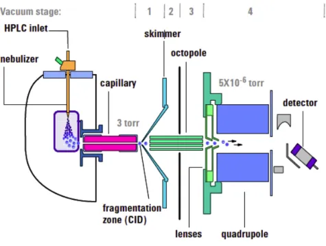
LC/MS platforms (also in its HPLC and UPLC configurations ) also consist of two differ-ent coupled analytical instrumdiffer-ents: a liquid chromatograph and a MS. LC/MS devices have been used widely in Metabolomics and they are probably one of the most widely analytical device used in metabolomic studies at the moment [13,16]. Figure1.1shows a scheme of a LC/MS experimental device. A liquid chromatograph uses a liquid as a mobile phase to transport the sample molecules through the chromatographic column. In Metabolomics, it is specially used the LC/MS setup having an Electrospray Ionisation (ESI) source and a TOF mass analyser. The molecules reaching the electrospray undergo a soft ionisation process called Electrospray Ionisation [8,17]. In general this ionisation does not break the molecules in the samples but it ionises them, allowing the creation of aggregates with the gain or loss of atoms or molecules. If the resulting aggregate has greater mass than the original molecule it is called an adduct and if it has lower mass, it is a fragment. ESI ionisers generate a great number of ions and they can be set up in either positive or negative polarisation modes. Depending on the characteristics of the molecule, it is easier ionised in the positive or negative polarisation set up. To obtain a complete metabolite profiling of the samples it is required to analyse the samples in both ionisation modes [11]. The reverse phase chromatograph set up is a usual choice when using an LC/MS platform in the Metabolomics context [11]. This configuration allows for suitable analysis of medium and low polarity metabolites. However, there are important metabolites like aminoacids or sugars that are hardly detected under this setup, as they elute in a very small retention time [11,18]. Due to this fact, it has been developed of a new type of LC/MS device called Hydrophilic Interaction LIquid Chro-matography (HILIC) that uses a special chromatographic column to detect this kind of

2

Figure 1.1: Diagram of an LC/MS device using a quadrupole as a mass analyser.

The model of the picture is a Agilent 6100 Series Quadrupole http://www.kprime.

net/pdf/products/6100_Data_Sheet.pdf

.

molecules [11,18]. It has been suggested that combining the output of the LC/MS with the HILIC might give a more complete profiling of the metabolites in the samples [11]. Typical single sample analysis in LC/MS in Metabolomics lasts for about 10-15 min [11].

In contrast to GC/MS, the samples need not to be derivatised prior to be analysed with a LC/MS device [14, 15]. Other advantages are a wider polarity range and molecular mass compared to GC/MS [15]. On the other hand, LC/MS sample analysis, as all MS-related devices, may suffer from ion suppression effect. This problem is related to the coelution of matrix components with the analytes affecting the device detection capabilities that is reflected in a drop of peaks intensities [11].

Bibliography

[1] Matt Ridley. Genome: The Autobiography of a Species in 23 Chapters. NY: Harper Perennial, New York, first edition, 2006. ISBN 0-06-019497-9.

[2] N. Leigh Anderson and Norman G. Anderson. Proteome and proteomics: New technologies, new concepts, and new words. ELECTROPHORESIS, 19(11):1853– 1861, 1998. ISSN 1522-2683. doi: 10.1002/elps.1150191103.

[3] S G Oliver, M K Winson, D B Kell, and F Baganz. Systematic functional analysis of the yeast genome. Trends in biotechnology, 16(9):373–378, 1998.

[4] Eva K. F. Chan, Heather C. Rowe, Bjarne G. Hansen, and Daniel J. Klieben-stein. The complex genetic architecture of the metabolome. PLoS Genetics, 6(11): e1001198, 11 2010. doi: 10.1371/journal.pgen.1001198.

[5] Venter J. Craig et al. The sequence of the human genome. Science, 291(5507): 1304–1351, 2001. doi: 10.1126/science.1058040. URL http://www.sciencemag.

org/content/291/5507/1304.abstract.

[6] David S. Wishart, Timothy Jewison, An Chi Guo, Michael Wilson, Craig Knox, Yifeng Liu, Yannick Djoumbou, Rupasri Mandal, Farid Aziat, Edison Dong, Souhaila Bouatra, Igor Sinelnikov, David Arndt, Jianguo Xia, Philip Liu, Faizath Yallou, Trent Bjorndahl, Rolando Perez-Pineiro, Roman Eisner, Felicity Allen, Vanessa Neveu, Russ Greiner, and Augustin Scalbert. Hmdb 3.0the human metabolome database in 2013. Nucleic Acids Research, 2012. doi: 10.1093/nar/ gks1065.

[7] E.J. Want, B.F. Cravatt, and G Siuzdak. The future of liquid chromatographymass spectrometry (lc-ms) in metabolic profiling and metabolomic studies for biomarker discovery. Biomark Med, 1(1):159–185, 2007.

[8] E.J. Want, B.F. Cravatt, and G Siuzdak. The expanding role of mass spectrometry in metabolite profiling and characterization. Chembiochem A European Journal Of Chemical Biology, 711:1941–1951, 2005.

[9] Katherine Hollywood, Daniel R. Brison, and Royston Goodacre. Metabolomics: Current technologies and future trends. PROTEOMICS, 6(17):4716–4723, 2006. ISSN 1615-9861. doi: 10.1002/pmic.200600106. URL http://dx.doi.org/10.

1002/pmic.200600106.

[10] Kermit K Murray. Glossary of terms for separations coupled to mass spectrometry. Journal of chromatography A, pages 209–212, 2010. URLhttp://www.ncbi.nlm.

[11] G. Theodoridis, H.G. Gika, and I.D. Wilson. Mass spectrometry-based holistic analytical approaches for metabolite profiling in systems biology studies. Mass Spectrometry Reviews, 30:884–906, 2011.

[12] G. Theodoridis, H.G. Gika, E.J. Want, and I.D. Wilson. Liquid chromatography-mass spectrometry based global metabolite profiling: a review. Analytica Chimica Acta, 711:7–16, 2012.

[13] Lu Xin, Zhao Xinjie, Bai Changmin, Zhao Chunxia, Lu Guo, and Xu Guowang. Lc-ms-based metabonomics analysis. Journal of Chromatography B, 866:64–76, 2007.

[14] Zhang Aihua, Sun Hui, Wang Ping, Han Ying, and Wang Hijun. Modern analytical techniques in metabolomics analysis. Analyst, 137:293–300, 2012.

[15] Vladimir Shulaev. Metabolomics technology and bioinformatics.Briefings in Bioin-formatics, 7(2):128–139, 2006. doi: 10.1093/bib/bbl012.

[16] Aur´elie Roux, Dominique Lison, Christophe Junot, and Jean-Fran¸cois Heilier. Applications of liquid chromatography coupled to mass spectrometry-based metabolomics in clinical chemistry and toxicology: A review. Clinical Biochem-istry, 44:119–135, 2011.

[17] John B. Fenn. Electrospray ionization mass spectrometry: How it all began.Journal of Biomolecular Techniques, 13(3):101–118, 2002.

[18] Zhou Bin, Xiao Jun Feng, Tuli Leepika, and Ressom Habtom W. Lc-ms-based metabolomics. Molecular BioSystems, 8:470–481, 2012.

State of the Art

Metabolomics has been the latest omic science (after genomics and proteomics) to undergo an important computational development in their data analysis workflows. Metabolomic studies apply experimental instruments and protocols devised in analyt-ical chemistry to biologanalyt-ical samples, with special emphasis in analysing biofluids and tissues [1]. Metabolomics aims at detecting and identifying low weight molecules (typ-ically under 1500-1800 Da) called metabolites [2,3] in biological samples under certain external conditions [4, 5,6]. Despite the fact that initially there were some differences between the terms Metabolomics and Metabonomics (see the classical Nicholson refer-ences [7, 8, 9]) the two terms are nowadays used interchangeably. In this thesis it will only be used the term Metabolomics.

There are two main approaches to perform Metabolomic studies depending on whether the metabolites to be detected are known (Targeted Metabolomics) or they are unknown (Untargeted Metabolomics) [3,4,10,11,12,13]. Performing a targeted or an untargeted metabolomic study is a critical issue for sample preparation [10], for the choice of the experimental setup [11] and for the statistical approach used [4, 10]. The basic under-lying difference between both types of study is that the main objective in Untargeted Metabolomics is to detect the highest possible amount of metabolites in the samples, whereas Targeted Metabolomics is only focused on detecting certain metabolites of in-terest.

2.1

Metabolomic Workflow

The main objective in Metabolomics is to study the metabolism using either quantita-tively or semi-quantitaquantita-tively approaches [1,3,13]. In metabolomic studies it is followed a well-established pipeline going from experiment design and statistical data analysis to biological interpretation of the results [1,3, 6,14]. Figure 2.1depicts the stages of the typical workflow for metabolomic studies. The main processing steps in a metabolomic analysis include the following stages:

• First steps are focused on an experimental context and they include the exper-imental design and collecting the biological samples. The samples are gathered following a sample protocol extraction [13,15]. The data acquisition is performed through analytical instruments such as an LC/MS or a Nuclear Magnetic Reso-nance (NMR) [4,11].

• Next stages include computational data processing steps such as peak detection, data filtering and data normalisation (Figure 2.1). One of the objectives of this stage for metabolomic untargeted studies is to obtain which peaks of the system are the most significant in terms of class separability in the data. That means to find which variables separate mostly separate the classes in the dataset. These classes usually refer to different study conditions like patients that have followed different diets or that have undergone some drug treatment. To find these signif-icant masses, the data are analysed through different statistical approaches [16] including multivariate and machine learning methods [3,17,18,19,20].

• The Statistical Analysis stage shown in Figure 2.1, might include a validation stage, whose objective is to evaluate the statistical predictive power contained in a subset of variables. Different Machine Learning techniques are applied in this stage being Partial Least Squares linear Discriminant Analysis (PLSDA) one of the most used approaches in Metabolomics [17].

• Peak annotation procedure is a processing step to improve the biological interpre-tation of the metabolomic data. This stage gives biological and chemical insight by labelling the variables (i.e. peaks) of the data with biological and/or chemical information. There are several kinds of peak annotation. Database mining is a type of peak annotation in which a database (or databases) are mined to match the

Figure 2.1: Metabolomic Workflow for Metabolomic Studies from Zhou et al [21].

peaks in the data to actual metabolites in the data. Another type of peak anno-tation step is the adduct or fragment identification depending on the polarisation used in the LC/MS instrument (see Section 2.2.5).

• Last steps of the workflow might include pathway and metabolic network analy-sis [1, 3]. Functional analysis is performed by searching for overrepresented and underrepresented labels from known biological data. In most metabolomic stud-ies, it is common to perform additional steps based on metabolite verification and quantification of the candidate metabolites (e.g. using a tandem MS for better metabolite identification) [3].

2.2

LC/MS Data Processing

The first data preprocessing steps after LC/MS data acquisition are signal filtering and peak picking, also known as peak detection (Figure2.1). The output of LC/MS instru-ments is a sparse 3D signal whose dimensions are intensity, m/z and the rt for each detected feature (peak mass). Figure2.2depicts an LC/MS profiling for a urine sample. The figure shows that the LC/MS signals are intrinsically sparse, as the majority of the 2D plane formed by m/z and rt does not contain any peaks. Furthermore, Figure 2.2

also shows that LC/MS signals are highly anisotropic. If we consider the integral of the whole signal in Figure 2.2 on the plane I-rt, the resultant signal has broader peaks and almost all the rt range has an intensity signal. On the other hand, the integral of the signal on the I-m/z plane gives narrow peaks and gaps in the m/z range without any intensity signal. This anisotropy is also depicted in the TIC shown in Figure 2.3

compared to the masses of Figure2.4

Peak mass signals can be recorded in either profile or centroid mode. Centroid mode records peak masses as a set of discrete values in which the peak masses have no width (Figure 2.4 shows a centroid mass recording). On the other hand, in profile recording the peak mass signal is continuous. Centroid mode recording produces smaller file sizes as only the peak centroid is saved. There are algorithms and tools provided by the commercial vendors of analytical devices to switch the signal recording from profile mode to centroid mode in a process called centroidisation [22].

2.2.1 Peak Detection

Peak Detection (also called Peak Picking) is a complex mathematical step that usually in-volve the use of complex peak detection algorithms and filtering methods [22,24,25,26]. The main objective of this step is to detect signal peaks which will ultimately be related to metabolites. The anisotropy of the LC/MS signals is exploited by many peak picking algorithms that detect the peaks taking into account that rt and m/z dimensions are different in terms of peak behaviour and peak resolution (m/z measures are more precise than rt measures) [24]. Two of the most used methods for peak detection are Matched

Figure 2.2: LC/MS profile for a urine sample from Guan et al [23]. The height

depicts the intensity in arbitrary units, horizontal axis is the m/z for the piece whereas the in-depth axis is the retention time in seconds

Figure 2.3: Chromatographic profile registered in a LC/MS device from Zhu et al

[27]. Horizontal axis is the retention time in minutes whereas the vertical axis is the

intensity measured in arbitrary units.

Filter [24,26] and centWave [22].

2.2.1.1 Matched Filter

Matched Filter method uses a two-fold differentiation approach and it has been one of the most widely used algorithms to filter LC/MS signals [26]. This method is implemented in the R package XCMS [24]. It makes the hypothesis that the chromatographic peaks can

Figure 2.4: Sample centroid spectrum profile registered from a urine sample in a

LC/MS device from Zhu et al [27]. Horizontal axis is the mass charge ratio in Dalton

whereas the vertical axis is the intensity measured in arbitrary units

be approximated by a certain function. It is usually assumed that the peak shapes are similar to a gaussian function. The next step is to perform a slicing of the signal known as binning in the m/z domain, and superimpose the second derivative of the gaussian function on the rt dimension of the signal to obtain a sharper chromatographic shape of the peaks [26]. XCMS software suggests taking a signal-to-noise cutoff value to finally detect the peaks once the filter has been applied [24]. This software tool also proposes to take the mean of the unfiltered data to determine the noise threshold value. The Matched Filter method shows some drawbacks related to having to manually choose the binning value, and to the dependence of the method with the gaussian function parameters [22]. If the binning value is too small, the m/z slices are so thin that the same chromatographic peaks are found in many slices and they are not detected as peaks. On the other hand, if the binning value is so large, small chromatographic peaks will not be detected as they will be added to other chromatographic peaks [22, 24]. The issue with the gaussian parameters is related to the different shapes that chromatographic peaks show in biological samples. Depending on the input parameters, the Matched Filter method can lead to detect more or less peaks than exist in the chromatogram due to the different shape between the input gaussian and the real chromatographic peaks.[22].

2.2.1.2 centWave

Another different approach is the centWave method which was specially design to avoid the binning problems associated to the Matched Filter algorithm. The centWave al-gorithm is based on detecting the so-called regions of interest (ROIs) in the centroided m/z domain, combined with a Continuous Wavelet Transform (CWT) approach for chro-matographic peak resolution [22]. Given a mass accuracy value, masses are classified to ROIs depending on their mass value. Regions with an amount of centroids below a user-defined threshold are removed. centWave method proposes the use of CWT to replace the second derivative of the Gaussian in the filtering as it correctly detects chro-matographic peaks of different width [22]. The CWT is applied to the extracted ion chromatogram and the local maxima of the coefficients are used to detect the chromato-graphic peak of the ROI [22]. Chronologically, the Matched Filter method was developed earlier than the centWave. Nowadays it is recommended to use the centWave method instead of the Matched Filter [28].

In a similar way than in the Matched Filter method, the centWave algorithm is also implemented in the XCMS package as another peak detection method.

2.2.2 Peak alignment

In a metabolomic study many biological samples are collected and analysed. A critical step in the metabolomic workflow is the a peak alignment stage. Computational data processing workflows typically include a transformation of the original raw data into a data matrix containing information of the peak masses and retention time values for all the samples [29]. This mathematical procedure requires the samples to be aligned in the retention time dimension to ensure that the retention time axis is the same for all the samples. The fact that the sample chromatograms may show different peak behaviour can have different reasons: replacement of the chromatographic column, changes in the mobile phase, drift in the instrument etc. [30]. Because of this wide variety of causes, the alignment procedure should consider possible unwanted non-linear effects in the reten-tion time [31]. Figure2.5shows how the chromatograms taken from consecutive samples may be unaligned. The objective of the alignment algorithms is to correct these effects

Figure 2.5: Group of unaligned LC/MS chromatograms the drift caused by an LC/MS

instrument, from van Nederkassel et al [32]. Each row corresponds to a sample and the

horizontal axis is the retention time. The lighter the colour, the higher the intensity of the signal.

and to get the same chromatographic peaks from all the samples as much aligned as possible. Ideally, after performing the peak alignment, the peaks of the resulting mean TIC chromatogram would have higher and sharper peaks thus improving the chromato-graphic behaviour of the samples as the uncertainty of the peaks would be lower.

The need for peak alignment in chromatography has been known for a long time and many alignment algorithms has been proposed [30,31,33,34,35,36,37]. The alignment algorithms can be divided into two main categories: those that require to run a peak mass detection stage prior to perform the alignment [38], and those algorithms that are applied directly on the chromatogram profiles without using the m/z values [30,37]. Among the most used methods for both types of algorithms there is the Locally Weighted Scatterplot Smoothing (LOESS) that uses peak masses and the Parametric Time Warping (PTW) that need not to detect the peak masses to run the chromatographic alignment.

2.2.2.1 LOESS

The LOESS method uses a warping approach using groups of well-behaved peak mass groups to adjust local polynomials and align the chromatograms [24]. To find the re-gression function, it is only used those points close to a certain pointx where we want

to evaluate the function [39]. The weight functions used in the LOESS algorithm are usually either quadratic or cubic polynomials. As a consequence, the LOESS algorithm performs the alignment of the chromatograms by performing a piecewise local adjust-ment of second- or third-order polynomials where the retention time intervals are found by detecting the groups of well-behaved peak mass groups. The LOESS method is also implemented in the XCMS package. The version implemented in the XCMS package uses high density peak regions considering all the samples to define the well-behaved peaks. When a group of samples show peak masses in a close region, it is likely that that peak is not much unaligned an is chosen as a well-behaved peak.

Despite being widely used in recent times and being implemented in a package like XCMS, LOESS method present the drawbacks of the warping methods. Being a piece-wise warping algorithm, the pieces of the chromatograms are stretched or compressed following the optimisation of an objective function. This warping procedure might cause artefacts in the aligned chromatograms or produce models with overfitting depending on the binning parameter.

2.2.3 Amplitude Normalisation

The next step in the LC/MS signal processing is the amplitude or intensity normal-isation. This stage corrects the overall changes in the intensity of the samples when different batches were used and/or because some samples were injected in different days and the experimental device shows a drift in the intensity measurements. Figure 2.6

depicts a PCA score plot of the LC/MS metabolomic data described in Wang et al [40]. In this plot it is shown that batch and injection order effects have an strong influence on the structure of the data by being and important source of variance in the data. In particular, the second PC of Figure 2.6 contains a combination of batch and injection order effects.

Batch effects cause the variables to behave differently depending on which sample is being considered. Because the sources of this misleading variance are many, the noise structure of LC/MS data have heteroscedastic behaviour, which means that signals with higher intensity values show higher variance [41]. As a consequence applying machine

Figure 2.6: PCA Scoreplot of the LC/MS data set from Wang et al [40]. Solid and open circles refer to WC and study samples respectively. Different colours are used to

label different batches. Solid lines show the injection order.

learning or multivariate methods such as PCA on the raw data may give wrong infor-mation [41] although these statistical methods has been applied in metabolomic studies for long time without normalising the intensity of the signal [18].

In recent years, many amplitude normalisation methods have been developed using dif-ferent approaches to the same problem [28, 40, 41, 42,43,44]. A number of them rely on the use of internal standards [28,42,44] to perform the intensity normalisation. The idea is that internal standards only undergo variations caused by the batch effects or time biases. The reason is that the internal standards are always the same samples so they do not contain biological variability (i.e. they will only show technical variability). As a consequence, if the internal standard for a certain sample shows a lower intensity value than a sample of the previous batch, it is expected that all the intensity levels for the samples of that batch (or that have been analysed closely in time to the QC) are going to show overall lower intensity values as well. These internal standards are usually called Quality Controls (QC) and typically can made of a pool of aliquots from all or a subset of the samples being analysed to ensure that they contain similar metabolic information[28]. Other QC strategies include using spikes or water samples as a control of the performance of the analytical instrument [18].

• LOESS method is used to correct the between-batch variations [28]. This method uses the QC peak expression to adjust a LOESS curve. As the QCs are injected in each batch, the LOESS adjustment measures the drift of the intensity across the time [28]. This curve is then used to correct the intensity values of the peaks for every sample.

• Veselkov et al. describes and compares the performance of four typical approaches to intensity normalisation with and without a variance stabilisation transformation that compensates the heteroscedastic noise of the LC/MS data [41]. The four tested approaches are LOESS, Median fold change (forces the median of log fold changes of peak intensities to be 0), Total Intensity (all samples are forced to have the same total intensity) and Quantile (forces the peak intensity distribution to be the same in all samples) normalisations. Their conclusions show that the best performance is reached by performing the variance stabilisation transformation and using the median fold change normalisation [41].

• A method called Batch Normaliser based in a linear regression model to normalise the intensity is proposed by Wang et al. [40]. The underlying idea of this model is to fit a linear model using the QC samples to capture the effects of both the batch and the injection order. Once the model is fit, the parameters of the model are used to correct the intensity of the rest of the samples [40]. In this paper, the Batch Normaliser method is compared to other standard methods like the quantile method. The results show that the Batch Normaliser outperforms all the methods tested.

2.2.4 Multivariate and Statistical Data Analysis

Once the features in the samples are detected (i.e. the m/z and rt for each peak), their chromatograms aligned and the intensity normalised, the next data processing stage is to perform the analysis of the data using Statistical or Machine Learning approaches. At this point the data takes form of a matrix with a row for each detected peak and a column for each analysed sample plus two more columns containing the m/z and rt data for each feature. The data of the matrix is the intensity of the peak for that sample. There are usually two different ways of computing this intensity which are the maximum

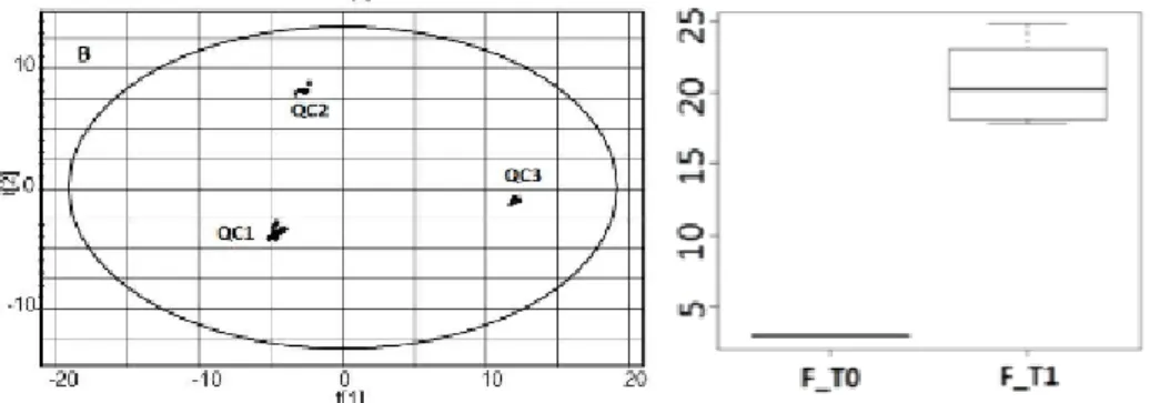
Figure 2.7: Left plot shows an scoreplot of QC samples analysed using an LC/MS

instrument. Right plot depicts a box plot of a single statistically significant feature of a dataset containing two classes (F T0 and F T1). Both plots are from Tulipani et al.

[45]

of the chromatographic peak or the area of the chromatographic peak [24].

Three main types of mathematical approaches might applied on this data matrix:

• A range of statistical tests such as parametric tests (e.g. Student’s t-test or ANOVA) or non-parametric tests (e.g. Mann-Whitney or Welch tests) are nor-mally applied on the data in order to obtain the most statistically significant features that separate the classes of the data [45]. As these tests are applied on each feature individually, the number of computed tests is high and performing a multiple test correction like Bonferroni or False Discovery Rate (FDR) is recom-mended to avoid false positives [46]. Plotting Boxplots (see the one shown in the right plot of Figure 2.7) is also a classical approach used in metabolomic studies to evaluate the differences of statistically significant features between the classes involved in the data. For example the box plot of Figure2.7shows that the plotted feature is statistically significant because the metabolite is found for samples of class F T1 but it is not found for both class F T0.

• The most common non-supervised technique applied on metabolomic LC/MS data is a PCA score plot of the data for visualisation purposes [47, 48]. Plotting the data in a PCA score plot allows a dimensionality reduction of the data and it revels the main sources of variance in the data. Left plot of Figure 2.7 depicts a 2D PCA score plot with three different types of QC samples. In this Figure it can be seen that the three classes are clearly separable in the PC1/PC2 plane as they appear depicted wide apart in the score plot. Another mathematical approach

Figure 2.8: Heat map showing the unsupervised clustering of samples at the top

(colours refer to real sample classification) and of the statistically significant features at the left side of the plot from Tulipani et al [45].

regarding non-supervised techniques are the unsupervised classifiers. In LC/MS metabolomic studies, unsupervised classifiers usually take the form of heat map plots in which are performed unsupervised clusterings of features and samples. Figure2.8depicts a heat map of samples having of two classes. The actual sample labelling is shown at the column colour at the top of the plot. The samples shown in the figure correspond to the statistically significant features found after performing a Student’s test on each feature. The most typical distances used for these hierarchical clustering are either the euclidean or the correlation distances. As it is clear from Figure2.8, heatmap figures are useful for analysing the results of metabolomic studies as they allow an easy correspondence of every significant feature to a class.

• Supervised classifiers such as PLSDA and SVM are normally used in an LC/MS metabolomic context to evaluate the class-related information of the features [47,

50, 49]. Repeated random sub-sampling cross-validation stages are applied us-ing SVM and PLSDA to evaluate the statistical predictive power of the LC/MS

Figure 2.9: Boxplot showing the classification ratio in a 50-fold random sub-sampling

cross-validation SVM classification stage from Nam et al [49]. The different boxes refer to different biomarkers used as variables to predict the samples.

metabolomic data. Figure 2.9shows the classification ratio of performing a cross-validation stage in a metabolomic study using four different biomarkers in SVM. Random forests can be used either as a supervised or unsupervised classifier and they are based on constructing sets of classification trees. The use of this technique in the LC/MS metabolomic context has increased in recent years [51].

2.2.5 Peak Annotation

Peak Annotation is a stage of the metabolomic data that has as an objective, to make the biological interpretation of the results easier by gaining some chemical and biolog-ical insight. In general, in LC/MS metabolomic data, the ionisation of a single source metabolite might give a set of features. To make easier the metabolite identification, there are some approaches that find the peaks coming from the same metabolite and relate them through possible chemical transformations that the molecules might have undergone in the MS. Depending on the polarisation mode used when analysing the samples, the peaks might form agglomerates with some other atoms or molecules, re-sulting in a overall charged positive (if the polarisation mode of the ESI was set to positive) or negative (if the polarisation mode of the ESI was set to negative) feature. The positively charged agglomerates are called adducts (for example if a sodium atom

was attached a piece of metabolite having neutral electrical charge) whereas the nega-tive are called fragments (for example if a hydrogen atom was removed from a piece of metabolite having neutral electrical charge). A typical approach to find these agglom-erated peaks is to define a retention time allowance window and a correlation threshold value [52,53,54]. Another agglomeration that the molecule pieces might undergo is the neutral loss or biotransformations, in which a neutral molecule is lost or attached to a piece of the ionised molecule (for example a loss of glucose from a a piece of metabolite having neutral electrical charge) [52].

Database mining can also be considered a type of peak annotation. Databases usually contain a relation between the metabolite and a primary mass i.e. a characteristic piece of the metabolite fragmentation or ionisation. To perform the metabolite identification step, the typical approach is using an allowance mass window to query a metabolite database for example METLIN [55] or Human Metabolome DataBase (HMDB) [21,27,

55, 56]. The main problem of this strategy is that, in general, the allowance window method is not restrictive enough and there are multiple possible hits for each query mass. Several approaches have been proposed to tackle this issue. A first approach to choose between several metabolite hit candidates, proposes to introduce a gaussian model in order to generate a probabilistic measure of the possible candidates [57]. Another approach is to used the so-called ”In silico fragmentation”. This strategy is based on performing the opposite procedure than the regular metabolite identification. The idea is to simulate the fragmentation pattern of the metabolites in the database following chemical laws and the check which of the simulated peaks appear in the real data [57,58]. As the final step of this procedure, the candidate metabolites are then ranked according to the number of matched peaks between the real and the simulated peaks.

2.3

Computational Tools

Analysing biological samples using an LC/MS in a metabolomic context produces high throughput data. Therefore, due to the sizes of the data involved in a typical metabolomic analysis, using software tools is a mandatory step in the data processing workflow. Many commercial brands producing their own LC/MS instruments, deliver their own in-house software tools with the analytical instrument. The softwares from Analyst http://

www.absciex.com/products/software/analyst-software or the software MarkerL-ynx from Watershttp://www.waters.com/waters/en_US/MarkerLynx-/nav.htm?cid=

513801&locale=en_US perform the first signal processing steps. There also exist

com-putational tools from companies focused on the statistical analysis of high-throughput data produced by such devices. These software tools are usually applied as black boxes with limited user intervention. Among these commercial computational tools, one of the most used softwares is SIMCA-P+ from Umetrics (http://www.umetrics.com/simca). Free tools usually developed in R [24], Python [59] or Java [60] to cite some, are also available and they are also widely used. R is a free software programming language specially focused on statistics with which have been developed many tools for analysing metabolomic data [61]. Besides R, in recent times it has been developed a great number of computational tools developed in many other programming languages like Python, Java or web tools. In this thesis, only free tools will be considered. Basically, the avail-able free tools fall within two different classes. There are tools which are specific of certain processing stages of the metabolomic data analysis workflow, like for example the CAMERA package which is focused on peak annotation (i.e. adduct, fragment and neutral loss annotation stages)[52]. Most of R packages fall within this category. Nev-ertheless more tools are needed to perform a complete complex metabolomic analysis when these kind of tools are used. On the other hand, there also exist free online tools that allow to perform a complete end-to-end metabolomic analysis such as Metaboan-alyst [62]. However, this kind of tools are usually implemented as a web service and they are not as flexible as the other set of tools due to its limited user customisation capabilities. Additionally, due to their web-based nature, it is hard to implement an automatic procedure to fully analyse the data with little user intervention. Table 2.1

contains a summary of the main available computational tools with their main stages of application in the metabolomic workflow.

2.3.1 R packages and other tools

R is perhaps the programming language in which the number of metabolomic packages is growing the most. Because of the package-based nature of the R language, newer R packages are normally supported on other older R packages. Therefore, the user can develop complex R packages with ease. Because of this feature of the R language, the

library of R packages which are focused on processing metabolomic data is increasing in number and complexity. Normally, the available R packages to perform metabolomic data analysis are focused on the first stages of the metabolomic workflow [24,52,53].

Among the available R packages in the metabolomic context, XCMS is one of the most used packages. The main tasks of this package are to perform the peak detection and peak alignment, as well as basic statistical processing in metabolomic data analysis. The package is designed to analyse signals from both GC/MS and LC/MS platforms. As it is explained in Sections2.2.1.1 and2.2.1.2, XCMS allows the use of both Matched Filter and centWave methods when it comes to filtering the raw signals and perform the peak detection stage. Before moving on to the peak alignment stage, XCMS groups the peaks across the samples. As it is said in section 2.2.2.1, Besides the LOESS method (explained in section2.2.2.1) to align the chromatograms, the XCMS package also con-tains other alignment methods such as Obiwarp [64] or the piece-wise linear alignment methods.

Besides the peak detection and peak alignment stages, XCMS also allows to perform basic univariate statistical tests such as ANOVA test (when there are more than two classes in the data) or a Student’s t-test (when there are two clases on the data) for each feature. The results of these statistical tests are retrieved as p-values in the output table of the package. Moreover, XCMS is able to perform and online query the Metlin database [55]. It was also published a protocol englobing the use of XCMS to perform the peak detection stage and the Metlin Database to identify the statistically significant features [27].

Another used package is CAMERA. This R package is designed to perform the peak annotation of adducts, fragments and neutral losses. The package requires the previous use of the package XCMS to detect the peaks before computing the peak annotation. It includes tables of adducts, fragments and neutral losses but it accepts a user-defined table as an input parameter to allow customisation of the peak annotations.

As it is explained in section 2.2.5, one of the methods to perform the peak annotation is to group the peaks using an allowance retention time window and a peak correla-tion threshold strategy. The Retencorrela-tion time allowance window is defined according to the shape of the chromatographic peak and a user input parameter. According to this procedure, the peaks falling inside the retention time allowance window are grouped as

possible candidates to come from the same source metabolite. In a second step, the correlation between the peaks of each group and across the samples is computed. If the correlation value is lower than a certain user-defined correlation threshold value, the group is split in groups where the peak correlation in the peak groups is equal or greater than the threshold.

In a similar way than the XCMS package, the output of the CAMERA analysis is a table. This table includes the XCMS output the peak annotation and also contains the peak groups obtained in the CAMERA workflow.

metaXCMS is another R package that proposes to perform an extra processing step besides the XCMS statistical tests [65,66]. The package is based on finding significant features between different pairwise experiments, giving as an the different combinations of statistical significant features in a Venn Diagram.

mzMine is a toolset implemented in Java and designed to analyse metabolomic signals [67]. The original mzMine launched in 2006 has been updated and improved recently to its second version mzMine 2.0 [60]. It performs the peak detection stage and basic statistical processing while the tool is designed putting emphasis on visualisation tools.

2.3.2 Online Computational Tools

Online Computational tools to perform metabolomic data analysis are a recent devel-opment compared to many software packages. Among the web tools available, Metabo-Analyst [62,68] and XCMS online [69] are two of the most widely used online tools for metabolomic data processing.

The first version of the MetaboAnalyst web server was launched in 2009 [68] but it has been updated recently to its second version [62]. Overall MetaboAnalyst is one of the most complete computational tools available for performing Metabolomic data analysis. It allows for and end-to-end processing workflow that analyse GC/MS, LC/MS and NMR metabolomic data. Among its processing steps, there are the data processing (including peak detection and noise filtering), data normalisation, statistical analysis (including

time-series analysis) and pathway/enrichment analysis [62]. A wide array of statisti-cal tools are available in the MetaboAnalyst 2.0 classified in traditional chemometric analysis including multivariate (like PCA, PLSDA) and univariate (ANOVA, t-tests) approaches or more advanced machine learning apporaches such as SVM or Random Forest methods. It also includes several methods to perform unsupervised clustering analysis like K-means or self-organising maps (SOM). Furthermore, MetaboAnalyst 2.0 has enhanced graphical interface compared to its first version making it more user-friendly. Before launching the second version of the MetaboAnalyst software tool, it was published a protocol to perform and end-to-end metabolomic analysis and obtain biological interpretation from raw data [70].

XCMS Online is another recently launched tool to perform end-to-end untargeted anal-ysis of metabolomic data. Its objective is to be an easy-to-use computational tool to analyse LC/MS data in a user-friendly environment [69]. XCMS Online uses the R package XCMS to perform the peak detection and peak alignment stage. The soft-ware automatically identifies the statistically significant metabolites using the Metlin database [69].

Table 2.1: Summary of the main available computational tools.

Tool Type Description and Functionality

XCMS R Package

Peak Detection, Statistical Test (Student’s T-test/ANOVA) and Metabolite Identification through Metlin Database query

CAMERA R Package

Peak Annotation of Adducts/Fragments and Neutral Losses. It complements the XCMS package.

metaXCMS R Package

Statistical Analysis. It complements the XCMS package by adding pairwise comparison of the significant features for pairs of experiments.

mzMine Java tool

Peak detection and basic statistical processing. Its main feature is the great range of visualisa-tion tools.

metaboAnalyst R Online Tool

The tool covers all the workflow, including peak detection, statistical analysis, peak annotation and pathway enrichment.

XCMS Online R Online Tool Peak detection, statistical analysis and Metabo-lite Identification through Metlin Database.

Bibliography

[1] Lu Xin, Zhao Xinjie, Bai Changmin, Zhao Chunxia, Lu Guo, and Xu Guowang. Lc-ms-based metabonomics analysis. Journal of Chromatography B, 866:64–76, 2007.

[2] Zhang Aihua, Sun Hui, Wang Ping, Han Ying, and Wang Hijun. Modern analytical techniques in metabolomics analysis. Analyst, 137:293–300, 2012.

[3] Zhou Bin, Xiao Jun Feng, Tuli Leepika, and Ressom Habtom W. Lc-ms-based metabolomics. Molecular BioSystems, 8:470–481, 2012.

[4] G. Theodoridis, H.G. Gika, and I.D. Wilson. Mass spectrometry-based holistic analytical approaches for metabolite profiling in systems biology studies. Mass Spectrometry Reviews, 30:884–906, 2011.

[5] E.J. Want, B.F. Cravatt, and G Siuzdak. The future of liquid chromatographymass spectrometry (lc-ms) in metabolic profiling and metabolomic studies for biomarker discovery. Biomark Med, 1(1):159–185, 2007.

[6] Aur´elie Roux, Dominique Lison, Christophe Junot, and Jean-Fran¸cois Heilier. Applications of liquid chromatography coupled to mass spectrometry-based metabolomics in clinical chemistry and toxicology: A review. Clinical Biochem-istry, 44:119–135, 2011.

[7] J. K. Nicholson, J. C. Lindon, and E. Holmes. ’Metabonomics’: understanding the metabolic responses of living systems to pathophysiological stimuli via multivariate statistical analysis of biological NMR spectroscopic data.Xenobiotica, 29(11):1181– 1189, November 1999. ISSN 0049-8254.

[8] J. K. Nicholson, J. Connelly, J. C. Lindon, and E. Holmes. Metabonomics: a platform for studying drug toxicity and gene function. Nat Rev Drug Discov, 1(2): 153–161, February 2002. ISSN 1474-1776.

[9] J. K. Nicholson and Wilson I.D. Understanding ’Global’ Systems Biology: Metabo-nomics and the Continuum of Metabolism. Nat Rev Drug Discov, 2(2):668–676, 2003.

[10] Nawaporn Vinayavekhin and Alan Saghatelian. Untargeted metabolomics. Cur-rent protocols in molecular biology edited by Frederick M Ausubel et al, Chapter 30 (April):Unit 30.1.1–24, 2010.