Distributed Inference and Query Processing for
RFID Tracking and Monitoring
∗Zhao Cao, Charles Sutton
†, Yanlei Diao, Prashant Shenoy
Department of Computer Science †
School of Informatics University of Massachusetts, Amherst University of Edinburgh
caozhao, yanlei, [email protected],
†ABSTRACT
In this paper, we present the design of a scalable, distributed stream processing system for RFID tracking and monitoring. Since RFID data lacks containment and location information that is key to query processing, we propose to combine location and containment infer-ence with stream query processing in a single architecture, with inference as an enabling mechanism for high-level query process-ing. We further consider challenges in instantiating such a system in large distributed settings and design techniques for distributed inference and query processing. Our experimental results, using both real-world data and large synthetic traces, demonstrate the ac-curacy, efficiency, and scalability of our proposed techniques.
1.
INTRODUCTION
RFID is a promising electronic identification technology that en-ables a real-time information infrastructure to provide timely, high-value content to monitoring and tracking applications. An RFID-enabled information infrastructure is likely to revolutionize areas such as supply chain management, healthcare, and pharmaceuti-cals [9]. Consider, for example, a healthcare environment such as a large hospital that tags all pieces of medical equipment (e.g., scalpels, thermometers) and drug products for inventory manage-ment. Each storage area or patient room is equipped with RFID readers that scan medical devices, drug products, and their associ-ated cases. Such an RFID-based infrastructure offers a hospital un-precedented near real-time ability to track and monitor objects and detect anomalies (e.g., misplaced objects) as they occur. The use of RFID tags provide similar benefits in distributed supply chains where objects, cases and pallets must be tracked, and in pharma-ceutical environments that require combating counterfeit drugs and preventing pilfering. To illustrate, consider the following types of continuous queries that may be posed on the RFID streams:
• Tracking queries, which include queries such as “report any pallet that has deviated from its intended path,” or “list the path taken by a medical device equipment through the hospi-∗This work has been supported in part by NSF grants IIS-0746939, IIS-0812347, and CNS-0923313.
Permission to make digital or hard copies of all or part of this work for personal or classroom use is granted without fee provided that copies are not made or distributed for profit or commercial advantage and that copies bear this notice and the full citation on the first page. To copy otherwise, to republish, to post on servers or to redistribute to lists, requires prior specific permission and/or a fee. Articles from this volume were invited to present their results at The 37th International Conference on Very Large Data Bases, August 29th - September 3rd 2011, Seattle, Washington.
Proceedings of the VLDB Endowment,Vol. 4, No. 5
Copyright 2011 VLDB Endowment 2150-8097/11/02...$10.00.
tal before it was misplaced.” Such tracking queries are loca-tionqueries that require object locations or location histories. • Containment queries,which include queries such as “raise an alert if a flammable item is not packed in a fireproof case,” or “verify that food containing peanuts is never exposed to other food cases for more than an hour.” This class of queries involve inter-object relationships, e.g., containment between objects, cases, and pallets, and are useful for enforcing pack-aging and shipping regulations.
• Hybrid queries,which include “for any temperature sensitive drug product, raise an alert if it has been placed outside a freezer and exposed to room temperature for 6 hours.” This class of queries combine sensors streams (e.g., temperature) and RFID streams (e.g., object location and containment) to detect various conditions.
Unfortunately, the nature of RFID data makes these queries dif-ficult to answer. The key challenge is that although such anomaly detection queries typically involve object locations and inter-object relationships such as containment, the RFID data does not directly contain this information. Rather, the data contains only the ob-served tag id and the reader id; this is a fundamental limitation of RFID technology. To enable queries on the data that is not actu-ally available, the key is to exploit statistical regularities in the tag id and reader information so that one canestimateobject locations and object relationships. The estimation problem is complex, how-ever, because RFID readings are inherently noisy due to the sensi-tivity of radio frequency to occluding metal objects and interference [7]. For example, in our lab setup (Section 5.2), we observed read rates of 70%-85% even with state-of-the-art readers and tags. Real deployments in complex environments such as hospitals would be expected to experience similar issues.
A second key challenge is that environments such as large hos-pitals or supply chains are distributed in scope, for which a central-ized approach may be limiting. In a centralcentral-ized approach, RFID streams from various readers are sent to a central location for query processing. This approach can fail to scale because of the band-width overheads incurred due to high data volume and can also potentially increase the latency of detecting anomalous events, es-pecially in geographically distributed settings. In contrast, a dis-tributed approach processes data streams as they emerge, thereby reducing the delay of answering queries. However, as objects move from one location to another, tracking and monitoring queries must also “move” with these objects. To do so, both the state of objects and the state of monitoring queries relevant to these objects must be transferred to the new location to seed the computation there.
Research contributions:In this paper, we present the design of a scalable, distributed stream processing system for RFID tracking and monitoring. Our system combines location and containment
inference with stream query processing into a single architecture, with inference as an enabling mechanism for high-level query pro-cessing for tracking, monitoring, and anomaly detection. We fur-ther scale such inference and thus enable query processing in large distributed environments that span multiple sites and numerous ob-jects. More specifically, our contributions include the following:
Novel statistical framework (Section 3). The key novelty in our approach to location and containment inference is to introduce the notion ofsmoothing over object relations, whereas all existing work on RFID data cleaning [8, 11] and location inference [14, 16] is limited to the traditional approach of smoothing over time. In contrast to temporal smoothing approaches, smoothing over con-tainment in our work leads to a much simpler graphical model, thereby allowing more efficient inference. At the same time, our model and inference techniques can still accurately estimate loca-tion and containment informaloca-tion, so that high-level query process-ing can return high-quality answers.
Our general approach is as follows: (i) Our probabilistic model describes a physical world comprising object locations, contain-ment relationships, and noisy RFID readings. (ii) We devise an in-ference algorithm, called RFINFER, for our model, working within an expectation maximization (EM) framework. The design of our model allows us to derive a simple customized M-step, which is essential for working at scale but still offers provable optimality. Furthermore, our algorithm is developed in anunsupervised learn-ingframework; that is, it does not use machine learning techniques that require access to any specially-generated training data. (iii) We finally extend our algorithm to also detect changes of contain-ment using a statistical method calledchange point detection.
Distributed inference and query processing(Section 4). To suit the increasing scale of RFID tracking and monitoring, we develop a distributed approach that performs inference and query process-ing locally at each location, but transfers the state of inference and state of query processing as objects move across sites. A naive in-ference algorithm would incur high transfer overhead by requiring the entire history of observations collected from multiple sites over a long period of time. Instead, we propose to truncate history by sifting out the observations most informative about the true con-tainment, and further distill such useful history into a few numbers for each object to minimize the inference state transferred. In dis-tributed processing of tracking and monitoring queries, the main issue is that we need to transfer one copy of query state for each object. Our work exploits the inference results, in particular, stable containment to share query state among objects.
Performance evaluation(Section 5). Our evaluation, using both real-world data and large synthetic traces, shows the following: (i) Our inference algorithm is highly accurate, with less than 7% er-ror on containment and 0.5% erer-ror on location, for noisy traces with stable containment. (ii) With containment changes, our algo-rithm can achieve 85% accuracy when read rates reach 0.7 while keeping up with stream speed, as shown using real lab traces and simulations. (iii) Our distributed inference method offers 3 orders of magnitude reduction in communication cost over a centralized method without compromising accuracy, and scales to millions of objects over multiple sites. (iv) Our highly accurate inference al-lows a query processor to produce high-quality answers and further exploit sharing of query state across objects for state migration.
2.
BACKGROUND
In this section, we provide background on RFID technology and RFID tracking and monitoring applications. Our system targets any distributed environment with multiple locations such as hospi-tals with multiple storage areas, supply chains with multiple
ware-houses, etc. For ease of exposition, the rest of this paper assumes that the environment is a distributed supply chain; however, our techniques are general and can be applied to other domains as well. Each item in the supply chain is assumed to be packed into a case, and multiple cases packed onto a pallet, which yields a containment relationship between items, cases and pallets. Items, cases, and pal-lets are assumed to be tagged. Each tag has a unique identity; the tag id can also indicate the level of packaging, e.g., a pallet, a case, or an item. We focus on passive RFID tags, which are battery-less and have a small amount of on-board memory, e.g., 4-64 KB. This memory is writable and can be exploited to store supply-chain-specific object state and enable “querying anytime anywhere”.1We assume that each distribution center employs multiple RFID read-ers, for example, at the entry and exit points as well as at the belt and shelves to scan resident objects. Each such reader periodically interrogate tags in its read range and immediately returns the sensed data in the form of (time,tag id,reader id). The local servers of a distribution center collect raw RFID data streams from all readers and process these streams. The data streams from different centers are further aggregated to support global tracking and monitoring.
We next illustrate the tracking and monitoring queries that our work aims to support. Such queries assume an event stream with rich information including (time, tag id, location, container) and optional attributes describing object properties, such as the type of food or type of container (which can be obtained from the man-ufacturer’s database). Note the different schemas for raw RFID readings and events used in query processing—events in the latter schema are produced by an inference module as we discuss shortly. Query 1 is an example of a hybrid query that combines object locations, containment relationships, and temperature sensor read-ings. This query raises an alert if a frozen food or drug product has been placed outside a freezer and exposed to room temperature for 6 hours. The query is written using the CQL Language [2] with an extension for pattern matching [1]. The inner (nested) query checks for each product if its container is not a freezer or does not exist, and if so retrieves the temperature based on the product’s location. The outer query aggregates the retrieved temperatures for the prod-uct and checks if it has been exposed to room temperature for 6 hours. The query finally returns all the temperature readings in the 6 hour period and the tag id of the object.
Q1:Select tag id, A[].temp
From ( Select Rstream(R.tag id, R.loc, T.temp)
From Products [Now] as R, Temperature
[Partition By sensor Rows 1] as T
Where (!(R.container IsA ‘freezer’)
or R.container = NULL) and R.loc = T.loc and T.temp > 0 °C ) As Global Stream S
[ Pattern SEQ(A+)
Where A[i].tag id = A[1].tag id and
A[A.len].time > A[1].time + 6 hrs ]
3.
INFERENCE ALGORITHM
In this section, we present our inference module that translates raw noisy RFID readings, (time, tag id,reader id), into high-level events with rich attributes (time,tag id,location,containe
-r) and optionally other attributes about object properties from the manufacturer. Our solution to this problem makes use of techniques from probabilistic reasoning, statistics, and machine learning.
1
This technology trend motivated us to minimize the computation state as-sociated with a tag, as discussed in Section 4, so it can be held in a tag’s local memory to enablequerying anytime anywherein the future.
Locations: Time Containers Objects A t = 1 1 3 4 2 5 6 B t = 2 1 3 4 2 5 6 C D t = 3 1 3 4 2 5 6 C E F t = 4 1 3 4 2 5 6 D E
Figure 1:Example of noisy RFID readings and containment changes Intuitively, the idea is that whenever an object is read, its con-tainer is likely to be read as well. Over time, we can use the co-location historyof containers and objects to derive the containment relationships. To develop this intuition into a robust system, how-ever, several design considerations must be addressed to effectively handle the noisy and incomplete input. To explain these considera-tions, we use the example in Figure 1: Each node represents a tag, and each edge a containment relation. The shaded nodes represent tags that were read (by the reader specified in the bottom row), and the unshaded nodes are tags that were missed by all readers.
A main design consideration is how to handle missed readings. If some objects are not observed, it is difficult to accurately de-termine their locations, which makes it also difficult to tell when objects are co-located. If the containment relations were known for certain, then a powerful way to determine object locations would be tosmooth over containment relations, meaning that whenever we read one object in a container, we know that all of the other ob-jects must be in the same place. For example, in Figure 1, at time
t= 3, we miss reading container 2, but we do read object 5. If we knew that container 2 contained object 5, then we could correctly infer that container 2 is also present at location C.
Unfortunately, the containment relationships are not known in advance, so instead we use aniterative approach. First, we start with the best available information about object locations and have a guess about containment relationships based on co-location. Then we can improve our understanding of object locations via smooth-ing over containment relationships. For example, in Figure 1, con-tainer 2 and object 5 are repeatedly co-located in the raw readings, so we can infer a containment relationship right away. Given the containment relationship, we can infer the location of container 2 att = 3. The resulting better understanding of locations allows us to further improve our understanding of containment relation-ships. Revisit Figure 1. We did not have strong evidence about the container for object 6, but with the new location information about container 2, we see that it is consistently co-located with object 6.
A second main design consideration is how to detect changes in containment relationships. Consider an object and a container that have been consistently co-located, such as container 1 and object 4 in the first two time steps of Figure 1. If later on (t = 3in the example), we fail to read the object, then following the idea of smoothing over containment, it is reasonable to infer than object 4 is still co-located with container 1. But at some point, if we repeat-edly fail to read the object (as att= 4), we may suspect that the object has actually been moved. To distinguish between these two competing explanations—either the object has been removed from the container, or it has not moved but its tag has been missed—we need a way to decide when there is enough recent evidence to con-clude that the containment relationship has actually changed. How much evidence is enough should depend on the read rate: if the readers are less accurate, then we ought to demand more evidence. We resolve all of these difficulties in a principled way using a general methodology based on graphical modeling. We design a graphical model that represents the probabilistic dependencies between the observed RFID readings and the latent object loca-tions and containment relaloca-tionships. Inference algorithms infer containment and locations in a unified way, naturally smoothing over the dependencies between them. In the following, we propose
... ... ... 1 2 R Container 1 Reader �t,c=2 ... ... ... 1 2 R Container 2 Reader �t,c=1 �t,o=1 �t,o=2 �t,o=3 �t,o=4
xt,c=1 yt,o=1 yt,o=2 xt,c=2 yt,o=3 yt,o=4 Figure 2:Graphical model of locations and RFID readings. a graphical model (Section 3.1) and a new algorithm RFINFER
(Section 3.2) for inferring containment and location from RFID readings. Containment changes can be further detected using a change point detection algorithm (Section 3.3). Moreover, infer-ence must run at stream speed, which poses a challenge to existing machine learning methods. The techniques we employ include op-timizations (Appendix A.3) and history truncation (Section 4).
3.1
Graphical Model
In this section we describe a probabilistic model of container locations, object locations, and RFID readings. The model is a probability distribution over random variables that represent both the true state of the world, which we do not observe, and the RFID readings, which we do. For the purposes of describing the model, we assume that we know the containment relationships exactly; in fact, we infer them from RFID data, as explained in Section 3.2.
We discretize both time and space: We divide time into a set of discrete epochsof, for example, one second in duration. All RFID readings that occur in the same epoch are treated as simulta-neous. As for locations, given the set of tracking and monitoring queries we aim to support, it suffices to localize objects to the near-est reader. Therefore, we model locations as a discrete setR, which is the set of locations of all of the static readers. Finally, we assume that there areC containers, denoted by integersc ∈ [1, C], and there areOobjects, denoted by integerso∈[1, O].
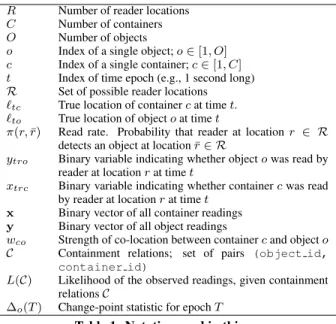
The random variables in the model are as follows. For each epocht, and each containerc, let`tc be the true location of the container. This is a random variable which takes values from the set of locationsR. Similarly, let`tobe the true location of each ob-jecto. As for the readings, letxtrcbe a binary random variable that indicates whether the reader at locationr ∈ Rreceived a reading of the containerc. Defineytrosimilarly for each objecto. To make the notation more compact, let`={`tc|∀t, c} ∪ {`to|∀t, o}be the vector of all the true object and container locations over all time, and similarly definex={xtrc|∀t, r, c}for the container readings andy = {ytro|∀t, r, o}for the object readings. The model is a joint distributionp(`,x,y)over all of these random variables.
Our model is depicted graphically in Figure 2 for a single epoch. To describe the model, we explain how to sample from the proba-bility distribution that describes the world, assuming that the world behaves exactly according to our model. At every epocht, first the true location`tcis sampled for each containerc. Because we do not assume any prior knowledge about the layout of the factory, we model this distribution as uniform over the set of all possible loca-tionsR. Now there is no need to sample object locations, because each object must be in the same place as its container.
Now we can generate the RFID readings. Each reader has aread rate, which we denoteπ(r,r¯), which is the chance of the reader at locationrreading an object which is actually at location¯r. Typ-ically, a reader detects an object if both are at the same location.
However, with a small chance a reader can detect an object that is closer to a nearby reader. In an actual deployment, one can measure the read rates periodically by using reference tags fixed to known locations and listening for these tags’ responses to a given number of interrogations [11, 16]. To create readings, each reader indepen-dently interrogates the tag on every container and the tag on every object. Formally, each binary observation variablextrcis sampled independently with probability according to the read rate; that is,
xtrcis true with probabilityπ(r, `tc). We write this probability as p(xtrc|`tc) =
(
π(r, `tc) ifxtrc= 1(tag read) 1−π(r, `tc) ifxtrc= 0(otherwise),
(1) and similarly forytro.
Putting it together, this defines ajoint probability distributionas
p(`,x,y) = T Y t=1 C Y c=1 p(`tc) Y r∈R p(xtrc|`tc) Y o|(o,c)∈C p(ytro|`to) (2) It can be seen that this model treats all time steps as independent and all containers as independent. For each epoch and container, it iterates over all readers and considers the probabilities of each reader observing the container as well as its contained objects. Be-cause the model treats all epochs as independent, it does not per-form any temporal smoothing over readings; however, it compen-sates for this by smoothing over containment relations instead. To smooth the readings over time as well would add significant com-plexity to the model, and significant computational cost to the in-ference procedure. In Section 5, we verify experimentally that smoothing over containment relations is effective at inferring ob-ject locations.
An important quantity is the probability that the model assigns to the observed data, that is,p(x,y) =P
`p(`,x,y). This quantity is called thelikelihoodof the data. Note that the likelihood is a function of the containment relationshipsC. To emphasize this, we defineL(C) = logp(x,y). According to our model, this is
L(C) = T X t=1 C X c=1 logX a∈R p(`tc) Y r∈R p(xtrc|`tc) Y o|(o,c)∈C p(ytro|`to) (3) The log likelihood measures how probable the RFID readings are under the current set of containment relationships. It will be an important quantity for inferring the containment relationships.
3.2
Inferring Containment Relationships
To infer containment relationships from RFID readings, we use a maximum likelihoodframework, that is, we determine the contain-ment relationships such that, according to the model, the observed readings are most likely. Formally, this amounts to maximizing the log likelihoodL(C)with respect to the set of containment relation-shipsC. In this section, we describe the algorithm that performs this maximization, which we call RFINFER.
The idea is that determining containment relationships would be simple if, besides the RFID data, we also observed the true loca-tions of all containers. However, the true container localoca-tions are in fact unknown. To handle this, we develop RFINFERin the EM framework, which offers a general approach for maximizing like-lihood functions in the presence of missing data, in our case the container locations. The algorithm alternates between two steps. In the first step, theexpectation step(or E-step), we infer a dis-tribution over the locations of each container, given some current guess about the containment relations. In the second step, the maxi-mization step(or M-step), we choose the best containment relations
given our current guess of the container locations. We iterate these two steps until the containment relations do not change.
In the E-step, the distribution that we want to compute is the conditional distributionp(`|x,y) over the location of each con-tainer that results from the joint distribution of Eq (3)—this distri-bution is called theposterior distributionof the container location and sometimes denoted asqtc(·)for simplicity. From the definition of conditional probability, it can be shown that
p(`tc|x,y) = S Y r∈R p(xtrc|`tc) Y o|(o,c)∈C p(ytro|`to), (4)
whereSis a constant that does not depend on`tc.
In the M-step, we update the current estimates of containment relationships based on the current belief about locations. We do so by defining a scorewcoto measure thestrength of co-location between objectoand containerc:
wco= T X t=1 X a∈R p(`tc=a|x,y) X r∈R logp(ytro|`to=a). (5) This score measures how likely are the readings of objectoif it were always co-located with containerc. To estimate the container foro, we simply pick the best containerC(o) = arg maxwco.
Note that RFINFERalso computes location information. When the algorithm has converged, the final values ofp(`tc|x,y)are our best estimates of the location of each container at each time step and the locations of objects believed to be in the container.
Finally, the following theorem states that our algorithm is guar-anteed to converge to an optimum of the likelihood:
Theorem 1. TheRFINFERalgorithm converges, and the resulting valuesC∗
are a local maximum of the likelihood defined in Eq(3). The proof is given in the Appendix A. The key step is to show that our simple, custom M-step indeed maximizes the likelihood.
Complexity, Optimizations, and Extensions.We refer the rea-der to the Appendix A for the complexity analysis, implementation, optimizations, and extensions of our algorithm. After a series of optimizations, our algorithm achieves a linear complexity,O(C+
O), in each iteration, and usually converges in just a few iterations.
3.3
Change Point Detection
In this section, we describe how we infer changes in contain-ment relationships. This type of problem, calledchange-point de-tection, is the subject of a large literature in statistics (see [3] for an overview). Achange point is a timetat which the contain-ment relationships change, that is, some object has either changed containers or been removed altogether. Finding change points is challenging because of the noise in RFID readings. For example, in Figure 1 att= 4, it may be unclear if object 4 has actually been removed from container 1, or it has simply been “unlucky” enough to be missed twice in a row. To distinguish these two possibilities, we need a way to quantify the unluckiness of a set of readings.
We propose a statistical approach based on hypothesis testing. Suppose that we have received readings from epochs[0, T]. Then we define anull hypothesis, which is that the containment relation-ships have not changed at all during epochs[0, T]. Then, if under the null hypothesis, it turns out that the observed RFID readings are highly unlikely, we reject the null hypothesis, concluding that a change point has in fact occurred. To measure whether the ob-served readings are unlikely, we again use the likelihood Eq (3). Consider a single objecto. LetC0:T be the maximum likelihood containment relations based on the full data, so that L(C0:T) is
State migration Objects (Tags) Inference Query Processing RFID readings (tag, reader, time)
Global Proc. Local Proc. Object events (tag, loc, cont, ...)
Site 2 Site 1 Site 3 Sensor readings State migration
Figure 3:A distributed RFID data management system. the best possible likelihood if there is no change point. Alterna-tively, suppose there is a change point at some timet0. Then let C0:t0 andCt0:T be the best containment relations that allow object oto change locations at timet0. Maximizing over possible change points, the best possible likelihood if there is any change point foro
ismaxt0L(C0:t0) +L(Ct0:T). We perform change point detection using the difference of these two log likelihoods, that is,
∆o(T) =L(C0:T)− max t0∈[0,T]
[L(C0:t0) +L(Ct0:T)] (6)
Essentially, this measures how much better we can explain the data if we use two different sets of containment relationships instead of one. This is a type ofgeneralized likelihood ratiostatistic, which is a fundamental tool in statistics. The change point detection pro-cedure will signal that there has been a change point whenever the value of∆o(T)is greater than a thresholdδ.
Intuitively, to choose the threshold we would like to know what values of∆o(T)would be typical if there were no change point. Fortunately, we can obtain as much of this data as we want, simply by sampling hypothetical observation sequences from the model, exactly as described in Section 3.1. Since none of the hypothetical sequences actually contain a change point, if our procedure signals a change point on one of them, it must be a false positive. In prac-tice, all of the hypothetical∆o(T)values are quite small, so we chooseδto be their maximum. Furthermore, all of this compu-tation can be done in advance before any RFID data is observed. The details of the change point detection procedure are given in Appendix A.2.
4.
DISTRIBUTED PROCESSING
As object tracking and monitoring systems grow into many geo-graphically separate sites and millions of objects, the sheer volume of data poses a scalability challenge. A centralized approach, like centralized warehousing, requires all the data to be transferred to a single location for processing. This approach incurs both delay of answering queries and high communication costs.
In this work, we propose a distributed approach natural for ob-ject tracking and monitoring, which performs“querying where an object (and data) is located”. The architecture of such a distributed system is illustrated in Figure 3. As can be seen, each site performs inference and query processing on local RFID streams as objects are observed. Inference runs on raw RFID streams and produces an object event stream describing the location and container of each object. Query processing runs continuously on the object event stream and other sensor streams to return all answers. Inference and query processing, however, often require information from the previous sites that an object has passed. To solve this problem, we performstate migration, which transfers the state of inference and query processing for an object when it moves across sites.
-160 -140 -120 -100 -80 -60 -40 -20 0 20 40 60 80 100 120 140 160 180 200
Cumulative Evidence (log)
Time t R NRC NRNC -160 -140 -120 -100 -80 -60 -40 -20 0 20 40 60 80 100 120 140 160 180 200
Cumulative Evidence (log)
Time t R NRC NRNC
(a)Cumulative evidence -4 -3 -2 -1 0 40 60 80 100 120 140 160 180 200
Point Evidence (log)
Time t R NRC NRNC -4 -3 -2 -1 0 40 60 80 100 120 140 160 180 200
Point Evidence (log)
Time t R NRC NRNC
(b)Point evidence
Figure 4:Evidence of co-location of three candidate containers. State migration can be realized in several ways: (i) When an ob-ject is scanned at the exit of a site, if domain knowledge about its next location is available, its inference and query processing state can be transferred directly to that site. (ii) Alternatively, when an object reaches a new site, the server there can locate the object’s previous place using the Object Naming Service (ONS) and re-trieves its state from that place. (iii) Finally, it is desirable to write the object’s state to the local storage of the RFID tag (once the tech-nology of writable tags matures for large deployments), while leav-ing a copy of the state at the current site as backup. This method will enablequerying instantly when a tag is in sight, with minimum delay of answering queries and minimum communication costs.
To reduce communication costs or cope with limited local tag storage, it is important to minimize inference and query processing state while ensuring accuracy of query answers. We address this issue in both inference and query processing as described below.
4.1
State Migration for Inference
Our inference algorithm presented in the previous section re-quires the entirehistory of readings associated with each object produced from all the sites that this object has passed. When an object leaves one site for another, the history of this object and the history of all of its possible containers, collectively called the infer-ence stateof the object, need to be transferred to the new location for subsequent inference. Evidently, transferring the complete his-tory of objects and containers would incur both a high communica-tion cost across sites and a high processing cost at the new locacommunica-tion. Below, we describe two techniques to address these problems.
Truncating History. The goal ofhistory truncationis to sift out the observations that are most informative about true contain-ment relationships from history, and retain only those for future processing. This can be accomplished by monitoring the strength of co-location computed in our containment inference algorithm RFINFER. Recall from Eq (5) for the M-step of the RFINFER algo-rithm, the co-location strengthwcofor each objectoand container cis a sum over all time steps of a quantity which we call thepoint evidenceof co-location. We denote this quantity by:
eco(t) = X a∈R qtc(a) X r∈R logp(ytro|`to=a). (7) Then thecumulative evidence of co-location can be computed as
Eco(t) =Ptt0=1eco(t0).
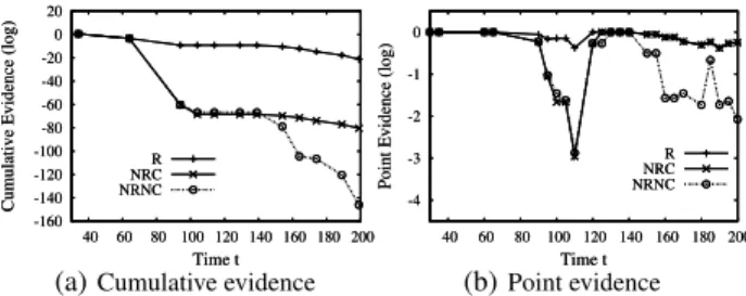
To see how these quantities are used, suppose that in a warehouse an object started at the entry door at time 0, was scanned on the con-veyor belt around time 100, and then placed on a shelf at time 150. Consider three candidate containers that were co-located with this object at the entry door: the real container (denoted byR) always traveled with the object; a second container (N RC) was co-located at the door and at the shelf, but not at the belt; a third container (N RN C) was not co-located after the door. Figure 4(a) shows the cumulative evidence of co-location of three candidate containers with the object. Around time 100, the belt reader scanned the real container alone with the object, causing the cumulative evidence of
the other two containers to drop fast. This is exactly the informa-tive region we want to find in history truncation. The information afterwards is less useful, because the false containerN RCis co-located with the object again on the shelf, while the false container
N RN Cwas already eliminated from contention by the belt reader. Our history truncation algorithm aims to find a time period, called thecritical region, whose observations are most informative for de-termining containment. While our intuition was explained using the cumulative evidence of co-location, our algorithm actually uses the point evidence of co-location, as shown in Figure 4(b) (in log space). During the critical region around time 100, the real con-tainer has much higher point evidence than the two false concon-tainers; this is not true either before or after the region.
After containment inference completes, our history truncation algorithm runs as follows: It searches through time by applying a small sliding window [t−w,t]. Given the current window, for each objecto, it computes the sum of point evidencePt
t0=t−weco(t0) for each possible container ofo. If the difference in sum between the best container and the second best is large enough (using a heuristic-based threshold), the current window is considered a crit-ical regionCRof the object, overwriting the previousCRif exis-tent. When the search reaches the end, the most recentCRis the final critical region of the object. Readings of the object and its possible containers outside the critical region will be all ignored.
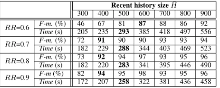
After running the algorithm, we have compressed the entire his-tory from [0,T] to a small regionCR. When the new readings arrive in the time period[T, T0], rather than running inference over the entire period[0, T0], we run inference only over the data in the the critical regionCRand in recent history denoted byH¯. If con-tainment is stable, it suffices to haveH¯ = [T,T0], i.e., including all new readings obtained since last inference. To support change point detection, however, we may need a somewhat larger recent historyH¯. According to Eq (6), the change point can be any point in the entire history. In practice, it is more likely to be in the recent history since it was not detected last time. However, it may be im-prudent to restrict the change point only to the most recent period [T, T0] because a change point before the timeT might not get sufficient evidence in the previous change point detection. Our ex-perimental results in Section 5.1 show that the sufficient size ofH¯
is within a factor of 2 ofT0-T. As time elapses, the recent history ¯
Hmoves forwards and we can truncate the readings falling behind ¯
Hby applying the critical region algorithm again.
Collapsing Inference State. When an object leaves a site for the next, theinference statefor the object includes the readings of the object and the readings of its candidate containers in both the critical regionCRand the recent historyH¯. One solution is simply shipping the inference state to the next site to seed inference there. However, the inference state for an object may not be small since each object can have dozens of candidate containers, and each container or object can have hundreds of readings inCRandH¯.
In our work we employ a technique to collapse the inference state to a single number for each container-object pair, i.e., the co-location weightwco, hence avoiding the overhead of transfer-ring readings entirely. This dramatically reduces the inference state transferred between sites. Then the inference algorithm at a new lo-cation simply adds the old transferred weights to the new weights that are computed from the readings at the new site. This technique, however, can affect accuracy: if later evidence shows that the con-tainment inference results from the old location were incorrect, we can no longer revise the old estimates as the corresponding read-ings have been discarded. Even in this case, however, inference in the new place still has a chance to correct the old estimates because readings obtained there will eventually overrule the old weights.
4.2
State Migration for Querying
Given an event stream with object location and containment in-formation, the query processor processes this stream and other sen-sor streams to answer monitoring queries. Our discussion below assumes CQL-based relational stream processing [2] extended with the pattern matching functionality [1].
Under our approach “querying where an object is located”, a monitoring query is registered with every site. It is split into local processing and global processing parts based on the labels of in-put streams specified in the query. For each query block, if any of the input streams is labeled as “global”, then this block uses global processing across sites; otherwise, it is processed only on the lo-cal streams. While lolo-cal processing can be performed by existing stream systems [1, 2], global query processing requires additional mechanisms. First, global query processing needs to maintain com-putation statefor each object. Since all stream systems maintain computation state (a.k.a. synopsis [2]) and update it with each ar-riving tuple, our work further partitions the state according to in-dividual objects. Then as an object leaves one site for another, we performstate migrationusing one of the three strategies mentioned at the beginning of the section. See Appendix B for illustration of the above approach using Query 1 in Section 2.
A main issue in state migration is that the total amount of state to be transferred can be enormous given a large number of objects. To reduce communication costs, we exploitstable containmentto share query states across objects. At the exit point of a storage area, we consider the objects in each container, e.g., frozen food prod-ucts considered in Query 1. These objects have the same container and location at present (but possibly different histories). The query states for these objects are likely to have commonalities. Hence, we propose a centroid-based sharing technique that finds the most rep-resentative query state and compresses other similar query states by storing only the differences. Details are available in Appendix B.
5.
PERFORMANCE EVALUATION
We have implemented a prototype of our inference approach, (in-cluding the optimizations in Appendix A), connected it to a stream query processor [1], and extended both to distributed processing. We evaluate our system using both synthetic traces emulating RFID-based supply chains and real traces from a laboratory setup.
5.1
Single-Site Inference
We first evaluate our inference algorithm on synthetic RFID stre-ams from a single warehouse. The detailed experimental setup, per-formance metrics, and additional results are given in the Appendix C. By default, we run inference every 300 seconds.
Inference with stable containment.We evaluate our inference algorithm first using traces with stable containment. To deal with traces of various lengths, we consider the Critical Region (CR) method that we proposed for history truncation in distributed pro-cessing (Section 4.1) as an optimization also for traces produced at a single warehouse. This method results in the use of the criti-cal region and a short recent historyH¯ (by default, the most recent 600 seconds) for inference. For comparison, we also include a sim-ple window-based truncation method that keeps the most recentW
readings for inference (W=1200 seconds here).
We first test the sensitivity of these methods to the read rateRR. As Figure 5(a) shows, while all three methods offer high accuracy for location inference (all three lines for location inference are very close, so we show only the line for Location(CR) for readability), they differ widely for containment inference: The window method has the worse accuracy because when the useful observations, such
0 2 4 6 8 10 0.6 0.7 0.8 0.9 1.0 Error Rate (%) Read Rate Containment(W1200) Containment(All) Containment(CR) Location(CR) 0 2 4 6 8 10 0.6 0.7 0.8 0.9 1.0 Error Rate (%) Read Rate Containment(W1200) Containment(All) Containment(CR) Location(CR)
(a)Basic (all history), fixed window, and history truncation methods with varied read rates
0 200 400 600 800 1000 1200 600 1200 1800 2400 3000 3600 Time cost (s) Trace length Inference(W1200) Inference(All) Inference(CR) 0 200 400 600 800 1000 1200 600 1200 1800 2400 3000 3600 Time cost (s) Trace length Inference(W1200) Inference(All) Inference(CR)
(b)Basic (all history), fixed window, and history truncation methods with varied trace lengths
20 40 60 80 100 0 20 40 60 80 100 120 F-measure (%)
Containment change interval RR=0.8 H=500 RR=0.7 H=500 RR=0.8 SMURF RR=0.7 SMURF
(c)Change point detection with varied anomaly frequencies (against SMURF∗)
0 5 10 15 20 25 30 T1 T2 T3 T4 T5 T6 T7 T8 Error rate (%) SMURF Cont. SMURF Loc. RFINFER Cont. RFINFER Loc. 0 5 10 15 20 25 30 T1 T2 T3 T4 T5 T6 T7 T8 Error rate (%) SMURF Cont. SMURF Loc. RFINFER Cont. RFINFER Loc.
(d)RFINFERvs. SMURF∗using real lab traces
0 5 10 15 20 0.6 0.65 0.7 0.75 0.8 0.85 0.9 0.95 1 Error rate (%) Read rate None CR Centralized 0 5 10 15 20 0.6 0.65 0.7 0.75 0.8 0.85 0.9 0.95 1 Error rate (%) Read rate None CR Centralized
(e)Distributed inference with varied read rates 0 5 10 15 20 20 40 60 80 100 120 Error rate (%)
Containment change interval None CR Centralized 0 5 10 15 20 20 40 60 80 100 120 Error rate (%)
Containment change interval None
CR Centralized
(f)Varied containment change intervals
Figure 5:Experimental results for single-site inference (a-c), our lab warehouse deployment (d), and distributed inference (eandf). as the belt readings, fall outside the window, the inference
algo-rithm can no longer use them to infer containment. Using the entire history or the CR method gives better accuracy as expected. Inter-estingly, while the CR method was initially proposed for improving performance, it also improves over the basic algorithm in accuracy due to the removal of noise (e.g., co-location of a false container and an object on a shelf) from inference. Moreover, its sensitivity to the read rate is comparable to that using the full history, which is the best that one can expect.
We next vary the trace length from 600 to 3600 seconds and compute the total inference time when using the entire history, the window, and the CR methods in Figure 5(b). Here we see that using the entire history severely penalizes the performance, the window based truncation stays in the middle, and the CR method performs the best with its running time insensitive to the trace length.
Containment change detection. We next employ the change point detection algorithm from Section 3.3 to detect containment changes. We use a recent history size ofH¯(600 seconds by default) in addition to the detected critical region for inference with change point detection. To generate events of interest, we inject anomalies that randomly choose an item and move it to a different case in the warehouse. The frequency of such anomalies is every 20 seconds by default but also varied over a wide range. Each run simulates a warehouse with 32,000 items in steady state over 4 hours.
Choice of threshold. We first examine the effect of the threshold
δfor change point detection. We consider fixed values in a range as well as our offline method as described in Section 3.3. Due to space constraints, the details of this study are left to Appendix C.4 (see Table 3). In summary, our chosen threshold always approximates the optimal value within 2% across all read rates.
Tradeoff between accuracy and efficiency. We further study the tradeoff between accuracy and efficiency. The change point detec-tion algorithm requires a recent history (whose size isH¯), besides the critical region in the past, to detect containment changes. Re-sults of our study show that a longer recent history helps improve accuracy especially when read rates are low, while it may increase inference cost. Overall, our algorithm can achieve 85% accuracy
given read rates≥0.7 while keeping up with stream speed (by us-ing a relatively smallH¯). The details are shown in Appendix C.4.
Frequency of unexpected containment changes.We next test the sensitivity of our algorithm to the frequency of unexpected tainment changes, i.e., without using special readers to scan con-tainers separately. We varied the interval between two containment changes, from 10 to 120 seconds. For comparison, we include an alternative method, called SMURF∗, that extends the state-of-the-art SMURF[11] method for RFID data cleaning with heuristics for containment inference (see Appendix C.3 for details). For our al-gorithm, we chose theH¯ size to keep up with stream speed based on Table 4 in Appendix C.4, i.e., H¯=500 for bothRR=0.7 and
RR=0.8. As Figure 5(c) shows, our algorithm is much more ac-curate than SMURF∗and is not very sensitive to the containment change interval. SMURF∗is much worse because it lacks a princi-pled approach to exploiting the iterative feedback between location and containment estimates.
5.2
Evaluation of Lab RFID Deployment
To evaluate our system in real-world settings, we developed an RFID lab with 7 readers and 20 cases containing 5 items each to simulate a small warehouse. We created 8 traces, labeledT1,. . ., T8, with different characteristics regarding the environmental noiseand overlap among readers (for details see Appendix C.2). We ran inference every 5 minutes using a 10-minute history (or all the data available if the history is less than 10 minutes). For comparison, we include the SMURF∗algorithm described in Appendix C.3.
Figure 5(d) shows the inference error rates for RFINFER and SMURF∗. As can be seen, RFINFER is much more accurate than SMURF∗across all traces although they both use intuitions such as smoothing and co-location. Again, this is because RFINFERuses smoothing over containment relationsand a principled approach for the iterative feedback between location and containment esti-mates. This is shown to be more effective than smoothing over time for individual objects and then combining such location evi-dence in a heuristic way to infer containment as in SMURF∗. For RFINFER, the location error rates are low across all traces. In the absence of containment changes, the containment error rates are
within 5% in tracesT1toT4despite the heterogeneous read rates,
added environmental noise, and significant overlap between read-ers. Containment changes cause containment error rates to rise, especially given lower read rates or higher overlap rates, but with a maximum of 13% with all the noise factors combined inT8.
5.3
Distributed Inference
Accuracy and Communication Cost. We next compare cen-tralized and distributed approaches to inference by simulating 10 warehouses for 4 hours. Each warehouse has 32,000 items in steady state, totally 0.32 million items. Our system runs inference at stream speed for each warehouse. Figure 5(e) shows the error rates for var-ied read rates. The naive no state-transfer method (labeled “None”) has a high error rate, while our critical region (CR) method perform close to the centralized method. Figure 5(f) shows similar results when the containment change frequency varies. The communica-tion costs (shown in Appendix C.5) show that our CR methods of-fer 3 orders of magnitude reduction in communication cost over a centralized approach while approximating its accuracy.
Scalability. We further test the scalability of our inference sys-tem by using larger numbers of objects in simulation. Our inference system can scale to 150,000 items per warehouse while keeping up with stream speed, totaling 1.5 million objects over 10 warehouses. The above reported results on accuracy and communication costs stay true. One way to support more objects is to use mobile readers for scanning objects on shelves (which is a more cost-effective de-ployment than static readers). In another simulation, we use a mo-bile reader to scan each isle of 90 shelves. The momo-bile reader reads every second and spends 10 seconds scanning each shelf. Given such reduced shelf readings, our inference system can scale to 1.21 million items per warehouse while running at stream speed, total-ing 12.1 million objects over 10 warehouses.
5.4
Distributed Inference and Querying
We finally extend our distributed inference experiment with query processing. We report results using two representative queries: Q1 from Section 2, and Q2 that reports the frozen food that has been exposed to temperature over 10 degrees for 10 hours. The table below reports the F-measure of query results and the total size of query state with and without the containment-based sharing method (Section 4.2). We see that the overall accuracy of query results is high (>89%). Also, state sharing yields up to 10x reduction in query state size. Finally, the accuracy and query state reduction ra-tio of Q1 are lower than those of Q2. This is because Q1 combines inferred location and containment, but Q2 only uses the inferred location which is more accurate than the inferred containment.RR=0.6 RR=0.7 RR=0.8 RR=0.9 Q1
F-m.(%) 89.2 94 95.1 96
State w/o share(bytes) 65,500 66,000 67037 67,000 State w. share(bytes) 6,986 5,737 5,589 5,156 Q2
F-m.(%) 93.5 96.1 97.3 97.5 State w/o share(bytes) 80,248 85,510 87,029 87,000 State w. share(bytes) 7,296 6,108 5,341 5,273
6.
RELATED WORK
RFID stream processing. Recent research has addressed RFID data cleaning [8] and location inference for static readers [11, 14, 4] and mobile readers [16]. However, containment inference is more challenging since inter-object relationships cannot be directly ob-served. Our work is the first to employsmoothing over object re-lationsin RFID inference, with demonstrated performance. Our work further supports distributed inference and querying.
RFID databases. Existing work has addressed RFID data archival [17], event specification and extraction [18], integrating data
cleans-ing with query processcleans-ing [13], and exploitcleans-ing known constraints to derive high-level information [19]. Our system addresses a differ-ent problem: it processes raw data streams to infer object location and containment, thereby enabling stream query processing, and scales inference and query processing to distributed environments. Inference in sensor networks.Various techniques [12, 6, 15, 10] have been used to infer true values of temperature, light, object po-sitions, etc., that a sensor network is deployed to measure. Our in-ference problem differs because the inter-object relationships, such as containment, cannot be directly measured, hence requiring dif-ferent statistical models and inference techniques. We further ad-dress distributed inference and query processing for scalability.
7.
CONCLUSIONS
In this paper, we presented the design of a scalable, distributed stream processing system for RFID tracking and monitoring. Our technical contributions include (i) novel inference techniques that provide accurate estimates of object locations and containment re-lationships in noisy, dynamic environments, and (ii) distributed in-ference and query processing techniques that minimize the com-putation state transferred across warehouses while approximating the accuracy of centralized processing. Our experimental results demonstrated the accuracy, efficiency, and scalability of our tech-niques. In future work, we plan to extend our work to include prob-abilistic query processing, exploit on-board tag memory to hold object state and enable anytime anywhere querying, and explore smoothing over object relations for other data cleaning problems.
8.
REFERENCES
[1] J. Agrawal, Y. Diao, et al. Efficient pattern matching over event streams. InSIGMOD, 147–160, 2008.
[2] A. Arasu, et al. The CQL continuous query language: semantic foundations and query execution.. VLDB J. , 15(2): 121-142, 2006. [3] M. Basseville and I. V. Nikiforov.Detection of Abrupt Changes:
Theory and Application. Prentice-Hall, 1993.
[4] H. Chen, W.-S. Ku, et al. Leveraging spatio-temporal redundancy for RFID data cleansing. InSIGMOD ’10, 51–62, 2010.
[5] N. N. Dalvi and D. Suciu. Efficient query evaluation on probabilistic databases.VLDB J., 16(4):523–544, 2007.
[6] M. Cetin, L. Chen, et al. Distributed fusion in sensor networks.IEEE Signal Processing Mag., 23:42–55, 2006.
[7] K. Finkenzeller.RFID handbook: radio frequency identification fundamentals and applications. John Wiley and Sons, 1999. [8] M. J. Franklin, S. R. Jeffery, et al. Design considerations for high
fan-in systems: The HiFi approach. InCIDR, 290–304, 2005. [9] S. Garfinkel and B. Rosenberg, editors.RFID: Applications, Security,
and Privacy. Addison-Wesley, 2005.
[10] A. Ihler, J. Fisher, et al. Nonparametric belief propagation for self-calibration in sensor networks. InIPSN, 225–233, 2004. [11] S. R. Jeffery, et al. An adaptive RFID middleware for supporting
metaphysical data independence.VLDB Journal, 17(2):265–289, 2007.
[12] M. Paskin, C. Guestrin, et al. A robust architecture for distributed inference in sensor networks. InIPSN, 55–62, 2005.
[13] J. Rao, S. Doraiswamy, et al. A deferred cleansing method for RFID data analytics. InVLDB, 175–186, 2006.
[14] C. R´e, J. Letchner, et al. Event queries on correlated probabilistic streams. InSIGMOD, 715–728, 2008.
[15] J. Schiff, D. Antonelli, et al. Robust message-passing for statistical inference in sensor networks. InIPSN, 109–118, 2007.
[16] T. Tran, C. Sutton, et al. Probabilistic inference over RFID streams in mobile environments. InICDE, 1096-1107, 2009.
[17] F. Wang and P. Liu. Temporal management of RFID data. InVLDB, 1128–1139, 2005.
[18] E. Welbourne, et al. Cascadia: a system for specifying, detecting, and managing RFID events. InMobiSys, 281–294, 2008.
[19] J. Xie, J. Yang, et al. A sampling-based approach to information recovery. InICDE, 476–485, 2008.
R Number of reader locations
C Number of containers
O Number of objects
o Index of a single object;o∈[1, O] c Index of a single container;c∈[1, C] t Index of time epoch (e.g., 1 second long)
R Set of possible reader locations
`tc True location of containercat timet.
`to True location of objectoat timet
π(r,r¯) Read rate. Probability that reader at locationr ∈ R
detects an object at location¯r∈ R
ytro Binary variable indicating whether objectowas read by reader at locationrat timet
xtrc Binary variable indicating whether containercwas read by reader at locationrat timet
x Binary vector of all container readings y Binary vector of all object readings
wco Strength of co-location between containercand objecto
C Containment relations; set of pairs (object id, container id)
L(C) Likelihood of the observed readings, given containment relationsC
∆o(T) Change-point statistic for epochT
Table 1: Notation used in this paper
APPENDIX
The notation used in this paper is summarized in Table 1.
A.
ENHANCEMENTS OF RFINFER
Below we present additional details about our inference algo-rithm, its implementation and optimizations, and two extensions.
A.1
Pseudocode and Proof of
RFINFERThe pseudocode for RFINFERis shown in Algorithm 1. We next prove Theorem 1 about the optimality of the RFINFERalgorithm. Proof. We show that RFINFER(Algorithm 1) is guaranteed to con-verge to a local maximum of the likelihoodL(C)in (3). Following the EM theory, we can interpret both the E-step and the M-step as maximizing a lower bound on the likelihood, which is
L(C)≥ T X t=1 C X c=1 X a∈R qtc(a) log p(`tc=a,x,y) qtc(a) =O(C)
The fact that this is a lower bound can be proven by Jensen’s in-equality. The E-step maximizes this bound with respect toqtc, and the M-step with respect toC. In RFINFER, the E-step is identical to the standard E-step of EM, but we use a custom M-step that is specific to our model. So it suffices to prove that the M-step in RFINFERindeed maximizesO(C).
When maximizing with respect toC, we can ignore terms that do not depend onC. ExpandingO(C)using Eq (3) and removing irrelevant terms yields
max C O(C) = maxC T X t=1 C X c=1 X a∈R qtc(a) X o|(o,c)∈C logp(ytc|`to=a) = max {c(o),∀o} O X o=1 wc(o),o,
wherec(o)denotes the container of objecto, andytc={ytrc|∀r}. In this last equation, notice that each containment decisionc(o)that we are maximizing over appears in only one term of the summa-tion. This means that we can find the global maximum by maximiz-ing each term independently, i.e.,maxCO(C) =Pomaxc0wc0,o. This is exactly what is computed in lines 12–20 of RFINFER.
Algorithm 1Pseudocode of RFINFERfor inferring containment whilenot convergeddo
//E step: compute newq
fort= 0toTdo//For each epoch forc= 1toCdo//For each container 5 for alla∈ Rdo//For all possible locations
qtc(a)← Y r∈R p(xtrc|`tc=a) Y o|(o,c)∈C p(ytro|`to=a) //Nowqtc(a) =S−1p(`tc=a|x,y) S←P a∈Rqtc(a)
for alla∈ Rdo//For all possible locations 10 qtc(a)←qtc(a)/S
//Nowqtc(a) =p(`tc=a|x,y) //M step: compute neww
foro= 1toOdo//For each object forc= 1toCdo//For each container 15 wco← T X t=1 X a∈R qtc(a) X r∈R logp(ytro|`to=a) //M step: compute new containment set
C ← ∅
foro= 1toOdo//For each object
c∗←arg max
c∈[1,C]wco 20 C ← C ∪ {(o, c∗)}
Computation Complexity. Each iteration of RFINFERrequires
O(T COR2)time, where byiterationwe mean a single execution of lines 2–20. This is due to two reasons. First, the computation ofqtc(a)in line 6 requiresO(OR)time, and is executedO(T CR) times by the outer loops. Second, the computation ofwcoin line 15 requiresO(T R2)
time, and is executedO(CO)times by its outer loops. This is the running time of a naive implementation of the algorithm; in Appendix A.3, we describe several optimizations that improve the performance significantly. Also, note that this is the computational complexity per iteration. In general, it is difficult to characterize the number of iterations required for EM to converge, because this depends strongly on characteristics of the unknown true distribution. However, we observe empirically that our infer-ence algorithm usually converges in just a few iterations.
A.2
Details of Change Point Detection
The change point detection procedure works as follows: First, before any data arrives, choose the thresholdδas described in Sec-tion 3.3. Then, the change point detecSec-tion is run after each time the RFINFERalgorithm runs, which also provides the null hypothesis. For each objecto, we compute
∆o(T) =L(C0:T)− max
t0∈[0,T][L(C0:t0) +L(Ct0:T)] If∆o(T) < δ, then there is no change point foro. Otherwise, if ∆o(T)≥δ, then we flag a change point at the timet0that achieved the maximum in Eq (6). Moreover, we disregard the data from 0. . . t0in all subsequent calls to the change point algorithm, so we do not flag the same change point more than once.
In implementation, this procedure incurs little extra cost beyond the computation in the RFINFERalgorithm. Recall that in the M-step of the RFINFER algorithm, the co-location strengthwcofor each objectoand containercis a sum over all time steps of a quan-tity that we call the point evidence of co-location, denoted
eco(t) = X a∈R qtc(a) X r∈R logp(ytro|`to=a).
The cumulative evidence of co-location isEco(t) =Ptt0=1eco(t0). The point evidence of objectoand containercat each timetis
memorized so it can be re-used to calculateL(C0:t0)andL(Ct0:T):
L(C0:t0) =Eco(t0)andL(Ct0:T) =PT
t=t0eco(t). If the change point is detected at timet0, we use the w0co =
PT
t=t0eco(t)as the new strength of co-location to get the new container for object
o. All the computation above is simply the sum of the point evi-dence memorized from the computation of the RFINFERalgorithm. Hence change point detection incurs little extra overhead.
A.3
Implementation and Optimizations
In this section, we sketch the main data structures and optimiza-tions that we use to implement the RFINFERalgorithm including the change point detection extension.
Data structures. We use a series of tables: (1) The read rate table (size: R×R) stores the read ratesπ(r,¯r). (2) Two history tables: one for container readingsx(size:T×R×C), and one for object readingsy(size:T ×R×O)(3) The posterior probability table (T×C×R) stores the posterior distributionqtc(a)over con-tainer locations. (4) The weight table (C×O) stores the co-location strengthswco. (5) Finally, the containment table (vector of length O) stores the container inferred for each object. Although the his-tory and posterior probability tables grow with time, in Section 4 we describe a history truncation method that reduces the memory requirement without sacrificing accuracy. Finally, many of these tables, especially the history tables, are sparse, i.e., most cells are 0, and so can be easily compressed to save memory.
Optimizations. We further employ several optimizations to im-prove inference efficiency. Recall from Appendix A.1 that both the E-step and M-step of our algorithm have the complexityO(T COR2). The E-step can be easily improved as each object is typically read in only a small number of locations and each container contains a small number of items. Since both of those are bounded indepen-dently ofRandO, the E-step can be improved by a factor ofOR2
(according to Eq (4)). Then the E-step requires onlyO(T C)time. Regarding the M-step, it can be easily improved by a factor of
R2
(according to Eq (5)) again because each object is typically read in only a small number of locations. Next, we propose an op-timization, calledcandidate pruning, to improve the M-step further toO(T O), eliminating the factor ofC. The idea is that in line 15, when computing the container that is most strongly co-located with a given object, it is probably safe to consider only containers that have been observed frequently with the object. So as a heuristic, we restrict the set of candidate containers to those that were most frequently co-located during the first several epochs. When testing for change points, we also include as candidates the most frequently co-located containers from recent epochs. Our experimental results show that candidate pruning is effective at reducing the time cost without affecting the accuracy.
We further propose amemorizationtechnique that avoids unnec-essary computation: If the set of objects in a container did not change in the previous EM iteration, then the location probabil-ities and co-location strengths for that container cannot change at the current iteration, so we can simply re-use the old values without any extra work. This optimization does not introduce any error.
Moreover, we can also use the history truncation method, de-scribed in Section 4 to truncate the history of sizeT, to a small critical region whose size is independent ofT. All of the above op-timizations combined finally reduce thecomplexities of the E-step and the M-steptoO(C)andO(O), respectively.
A.4
Extensions to the
RFINFERAlgorithm
Missing container tags:We have assumed that we know a priori which tags are container tags and which tags are object tags, which
is typically true according to the EPC tag data standard2. Relaxing this assumption is possible. First, if the containers do not have tags, we simply omit the nodes in the graphical model that correspond to the readings from the container tags, along with the corresponding terms in Eq (4) and in line 6 of Algorithm 1. Alternatively, if all containers and objects have tags, but we do not know which are which, we treat all tags (for containers and objects) as if they were object tags; we use latent and evidence variables in the graphical model to denote the true and observed locations of these objects, respectively. Then, we use another copy of latent variables, `tc, to represent real containers and use them to encode containment relationships with objects. Eq (4) and Algorithm 1 are modified the same as above. We do not further optimize these cases because they are rare given the wide adoption of the EPC tag data standard. Hierarchical containment:Just as objects are grouped into con-tainers, containers may themselves be stored in larger concon-tainers, such as pallets. We can extend our model and algorithms to arbitrar-ily nested containment hierarchies, intuitively by adding latent vari-ables for the pallet locations whose values are imputed using EM in a similar way as the container locations. Since common types of queries such as those listed in Section 1 rely mainly on the imme-diate containers of items that are subject to shipping and packaging regulations, we defer a detailed study of hierarchical containment to future work when new applications requiring so emerge.
B.
DISCUSSION OF QUERY PROCESSING
We next describe our distributed query processing approach more. First, we illustrate our approach using Query Q1 in Section 2. A monitoring query is split into local and global processing based on the labels of input streams of each query block. For instance, for Query 1, the inner query block takes two streamsRandT. Neither of them is labeled as “global”, so this block is treated as local pro-cessing only. However, the output streamSof the inner query block is labeled as “global”, and hence the outer query block consuming
Sis considered for global processing. For global query processing, the computation state is recognized and partitioned for individual objects. Revisit Q1. The outer query block employs pattern match-ing on the stream produced by the inner block. An automaton-based query processor [1] defines the query state to be: (i) the cur-rent automaton state, (ii) the minimum set of values needed for future automaton evaluation, e.g., the tag id and the time of its first exposure to room temperature for Q1, and (iii) the values that the query returns, e.g., the tag id and the sequence of temperature read-ings for Q1. Partitioning the query state for objects is simply based on the tag id. Then as an object leaves one site for another, we per-formstate migrationby shipping the query state for this object to the next site or writing the query state into the tag’s memory.
Second, we propose to exploitstable containmentto share query states across objects. Our centroid-based sharing technique works as follows. LetQodenote the query state for objecto. We choose the most representative query state (the centroid) of allQo’s based on a distance function that counts the number of bytes that differ in the query state of two objects. The centroid selection problem has aO(n2)complexity, but since each case contains a limited number of objects, e.g., 20-50, this computation cost is modest on a mod-ern computer. Given the centroid, we compress the query states of other objects based on the distance to the centroid.
C.
ADDITIONAL EXPERIMENTS
In this section, we describe additional experimental results be-yond the key results presented in the main body of the paper.
2
Table 2:Parameters used for generating RFID streams.
Parameter Value(s) used
Number of warehouses (N) 1 - 10
Frequency of pallet injection (fixed) 1 every 60 seconds Cases per pallet (fixed) 5
Items per case (fixed) 20
Main read rate of readers (RR) [0.6, 1], default 0.8 Overlap rate for shelf readers (OR) [0.2, 0.8], default 0.5 Non-shelf reader frequency (fixed) 1 every second Shelf reader frequency (fixed) 1 every 10 seconds Frequency of anomalies (F A) 1 every 10 - 120 seconds
C.1
Experimental Setup
We developed a simulator using CSIM to emulate an RFID-based enterprise supply chain. The parameters are shown in Table 2. Each supply chain arrangesN warehouses in a single-source directed acyclic graph (DAG). Pallets of cases are injected at the source, and then move through a sequence of warehouses with a sched-uled delay in each warehouse and schedsched-uled transit time between two warehouses, until they reach final destinations. Our simulator guarantees that in a period of time, pallets arrive at a warehouse and depart from it at the same rate (i.e., the system is in steady state).
Within a warehouse, pallets first arrive at the entry door and are read by the reader there. They are then unpacked. By default, each warehouse has a reader at the conveyor belt that scans the cases one at a time. The cases are then placed onto shelves and scanned by the shelf readers. After a period of stay, cases are removed from the shelves and repackaged. The assembled pallets are finally read at the exit door and dispatched to subsequent warehouses in a round-robin fashion. In the simulation, all readers have a read rateRR
for its location, uniformly sampled from [0.6, 1] unless stated oth-erwise. There is significant overlap between adjacent shelf readers: a shelf reader can read objects in a nearby location with probability
ORuniformly sampled from [0.2, 0.8]. Finally, to stress test our containment change detection algorithm, our simulator can inject anomalies that randomly pick an item and place it in a different case, with the frequency specified by the parameterF A.
Our evaluation uses the following metrics:Error rate(%): To measure accuracy, we compare the inference results with the ground truth and compute the error rate. F-measure: For change point detection, we evaluate the accuracy of the reported changes. We useprecisionto capture the percentage of reported changes that are consistent with the ground truth, andrecallto capture the per-centage of changes in the ground truth that are reported by our al-gorithm. We combine them intoF-measure=2∗precision∗ recall/(precision+recall). Running cost: We report the time taken to evaluate a trace using a single-threaded implementation running on a server with an Intel Xeon 3GHz CPU and running Java HotSpot 64-bit server VM 1.6 with maximum heap size 1.5GB.
C.2
Lab RFID Deployment
To evaluate our system in real-world settings, we developed an RFID lab with 2 ThingMagic Mercury5 readers connected to 7 circularly-polarized antennas, 20 cases containing 5 items each, and Alien squiggle Gen 2 Class 1 tags attached to all cases and items. We used the 7 antennas to implement 1 entry reader, 1 belt reader, 4 shelf readers, and 1 exit reader. Cases with contained items transitioned through the readers in that order, receiving 5 interrogations from each nonshelf reader and dozens from a shelf reader. The shelf readers had overlapping read ranges as they were placed close to each other. Using our lab setup, we created 8 traces with distinct characteristics, by varying the environmental noise, overlap among readers, and tag orientations:
0 2 4 6 8 10 0.6 0.65 0.7 0.75 0.8 0.85 0.9 0.95 1 Error Rate (%) Read Rate Containment Location 0 2 4 6 8 10 0.6 0.65 0.7 0.75 0.8 0.85 0.9 0.95 1 Error Rate (%) Read Rate Containment Location
(a)Basic algorithm
0 2 4 6 8 10 600 1200 1800 2400 3000 3600 Error Rate (%) Trace length Containment(H) Containment(CR) Containment(W1200) 0 2 4 6 8 10 600 1200 1800 2400 3000 3600 Error Rate (%) Trace length Containment(H) Containment(CR) Containment(W1200) (b)History truncation
Figure 6: Experimental results for single-site inference
• T1 (RR=0.85, OR=0.25) represents the case of high read
rates, an average of 0.85 across readers, and limited overlap rates, an average of 0.25 for shelf readers using low power. • T2(RR=0.85,OR=0.5) is case of high read rates and
signif-icant overlap rates (using high power), an average of 0.5. • T3(RR=0.7,OR=0.25) involves lower read rates due to added
environmental noise, i.e., a metal bar placed on each shelf that is 1/3 the length of the shelf.
• T4(RR=0.7,OR=0.5) further has higher overlap rates.
• T5toT8extendT1toT4, respectively, with containment
chang-es. When all 20 cases were placed on shelves, 3 items were moved from one case to another and 1 item was simply re-moved, causing containment changes in 35% of the cases. We also obtained traces with varied tag orientations but observed little impact of this factor. This verifies that squiggle tags are orienta-tion-insensitive when used with circularly-polarized antennas.
C.3
Alternative Method for Comparison
We describe the design of the SMURF∗method used as