Chatter avoidance via structural modification of tool-holder geometry

(1)

This is a repository copy of

Chatter avoidance via structural modification of tool-holder

geometry

.

White Rose Research Online URL for this paper:

http://eprints.whiterose.ac.uk/154116/

Version: Published Version

Article:

Gibbons, T.J., Ozturk, E., Xu, L. et al. (1 more author) (2019) Chatter avoidance via

structural modification of tool-holder geometry. International Journal of Machine Tools and

Manufacture. 103514. ISSN 0890-6955

https://doi.org/10.1016/j.ijmachtools.2019.103514

[email protected]

https://eprints.whiterose.ac.uk/

Reuse

This article is distributed under the terms of the Creative Commons Attribution (CC BY) licence. This licence

allows you to distribute, remix, tweak, and build upon the work, even commercially, as long as you credit the

authors for the original work. More information and the full terms of the licence here:

https://creativecommons.org/licenses/

Takedown

If you consider content in White Rose Research Online to be in breach of UK law, please notify us by

(2)

International Journal of Machine Tools & Manufacture xxx (xxxx) xxx

Please cite this article as: Tom J. Gibbons,International Journal of Machine Tools & Manufacture, https://doi.org/10.1016/j.ijmachtools.2019.103514

Available online 2 December 2019

International Journal of Machine Tools and Manufacture

journal homepage:www.elsevier.com/locate/ijmactool

Chatter avoidance via structural modification of tool-holder geometry

Tom J. Gibbons

a

_{, Erdem Ozturk}

b

_{, Liangji Xu}

c

_{, Neil D. Sims}

a,∗

a_{Dynamics Research Group, Department of Mechanical Engineering, The University of Sheffield, Mappin Street, Sheffield S13JD, United Kingdom} b_{Advanced Manufacturing Research Centre with Boeing, The University of Sheffield, Wallis Way, Catcliffe, Rotherham S60 5TZ, United Kingdom} c_{The Boeing Company, Materials and Process Technology, 2400 Perimeter Road, Auburn, Seattle, WA 98001, United States}

A R T I C L E I N F O

Keywords: Chatter Milling Structural modification Tunable-mass Tool-holder

Receptance coupling substructure analysis

A B S T R A C T

Chatter is a self-excited vibration that can occur during milling operations causing undesirable consequences such as poor surface finish and increased levels of tool wear. One possible solution to this problem is to optimise the dynamics of the machine by tuning parameters such as tool stickout length, e.g. by using receptance coupling substructure analysis. Unfortunately, experimental limitations of the method, such as the requirement to model interface dynamics and the inefficient optimisation process, have hindered its advancement to the industrial sector.

This paper looks to resolve these issues by proposing a new structural modification method for chatter avoidance. Firstly, tool-holder diameter is investigated as a potential tuning parameter: a new experimental dataset demonstrates that this design parameter can have a significant and valuable impact on the chatter stability. Secondly, the direct structural modification method is introduced, allowing the tool-holder diameter to be modelled without any knowledge of the interface behaviour between tool and tool-holder. Thirdly, the inverse structural modification method is proposed, allowing tuning and stability optimisation by solving a single equation. Lastly, a new tunable-mass tool-holder is presented, allowing the dynamics of a milling machine to be tuned for each tool diameter and length range with a single tool-holder. This eliminates the need for manufacturers to purchase a wide range of tool-holders, a significant financial investment.

1. Introduction

High speed machining operations, such as milling, are widely used in many industries such as the aerospace sector. However, in these processes unstable self-excited vibrations, known as regenerative chat-ter, can occur due to the dynamic interaction between the tool-tip and the surface being machined. This has undesirable consequences such as poor surface finish, rapid tool and machine wear, as well as high noise levels; all of which lead to a reduction in the material removal rate (MRR). Efforts to avoid the onset of chatter are, therefore, of great importance to both academic and industrial engineers alike.

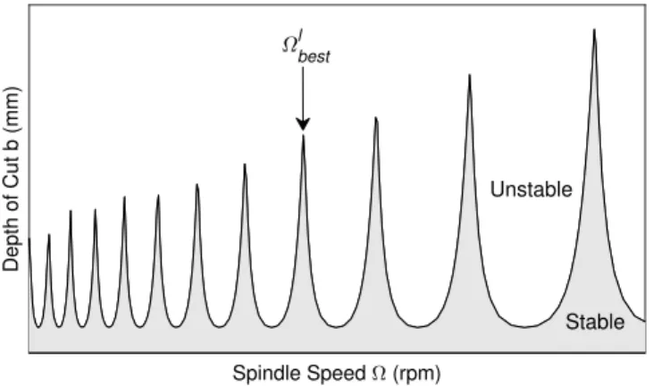
The onset of chatter in milling can be parameterised by the cut-ting parameters axial depth of the cut (b) and spindle speed (�),

and it is well known that this relationship is strongly influenced by the structural dynamics of the complete machine tool system [1,2]. With reference to the schematic example in Fig. 1, chatter can be avoided whilst still maximising the material removal rate by simply selecting a cutting parameter combination in one of the stable peaks in the Stability Lobe Diagram. However, if any parameter is changed, a new experimental model must be captured and the stability analysis repeated.

∗ _{Correspondence to: Department of Mechanical Engineering, The University of Sheffield, Sheffield, S1 3JD, United Kingdom.} E-mail address: [email protected](N.D. Sims).

Passive chatter avoidance is an active research field with many new methods still being proposed. These methods look to optimise the stability threshold by tuning some structural parameter of the machine and a good review of such methods can be found in [3]. By changing the structure’s dynamics, the stability threshold can be optimised for a given operation. For instance, it can be shown that the locations of the stable peaks (��

��inFig. 1) are directly proportional to the natural frequency of the machine [4],

�_�� = ��

2�(�+ 1)�_� (1)

where�_� is the natural frequency of the tool in rad/s,�∈ 0,1,2,…is the lobe number, and�_�is the number of teeth on the tool. Therefore, the location (or spindle speed) of the stable peaks can be optimised via the dominant natural frequency of the machine. Then, by tuning some structural parameter that controls this natural frequency, a stable peak can be re-positioned to a more desirable spindle speed — perhaps the maximum speed of the machine. Some of the more common tuning parameters include, the stickout length of the tool [5], the helix angles of the tool [6] and the bearing stiffness [7]. One such parameter that

https://doi.org/10.1016/j.ijmachtools.2019.103514

(3)

Nomenclature

� Geometric parameter

�_� Proportional damping coefficient

� Frequency (rad/s)

�_� Natural frequency (rad/s)

�_�� Desired natural frequency (rad/s)

�_� Mode shape for mode�

� Spindle speed (rpm)

�_�� Desired spindle speed (rpm)

� Axial depth of cut (mm)

� Lobe Number

�_1,...,4 Nodes 1 to 4

�_� Location of node�at base of adapter

�_� Location of node�at end of adapter

�_� Location of node�at tool tip

� _{Dynamic stiffness of model}_�

� Damping matrix

� Frequency response function matrix

� _{Identity matrix}

� _{Stiffness matrix}

� _{Mass matrix}

� Harmonic force vector

� Harmonic displacement vector

�_�� Frequency response function

�_�� Radial cutting force coefficient (MPa)

�_�� Tangential cutting force coefficient (MPa) �_�� Frequency response function

�_� Number of Teeth on Tool

�_�� Frequency response function

�_�� Frequency response function Subscripts

…_� Subsystem (machine & tool-holder) …� Subsystem (modification to tool-holder) …� Subsystem (assembled system)

…� Modified degrees of freedom

…� Unmodified degrees of freedom

…_� Degrees of freedom

…� Degrees of freedom

has received little attention is the tool-holder geometry, despite it being a relativity simple structure with significant potential to influence the stability threshold [8]. Therefore, this will form the main focus of this paper.

In practice, tuning the geometry of a tool-holder (or indeed any other geometrical parameter) would usually involve performing an experimental modal analysis on each tool-holder available to the user, calculating the stability of each, and selecting the optimum geometry. In order to streamline this process, the receptance coupling substruc-ture analysis (RCSA) method was proposed [9–11], [12–14]. RCSA is an application of dynamic sub-structuring to passive chatter avoidance. The aim of the method is to predict the dynamics of a machine with var-ious tools and tool-holders from a single experimental model, allowing the user to select the optimal set-up without having to perform multiple experimental modal analyses. This involves experimentally modelling

the dynamics of the complex spindle structure, and coupling this with a model of the simpler tool and tool-holder structures.

However, in previous methods, the coupling methodology relies heavily on the accurate modelling or calculation of the interface proper-ties between the tool and tool-holder, and between the tool-holder and spindle. This has proved difficult in practice [15,16], perhaps because the tool to tool-holder interface transmits significant machining forces and can exhibit load-dependent nonlinear behaviour. Moreover, the method does not lend itself easily to optimisation. In order to select the optimal tool-holder geometry, for example, the user must construct multiple numerical models for each and every geometry available, an exercise that can easily become costly. The approach can work well when the cutting tool is long and thin, but in other cases the structural dynamics are more strongly influenced by the spindle shaft and bearings, so that adjustments to the tool geometry are less effective. Furthermore, there are some practical scenarios where the tool stickout length cannot be tuned to the desired value, due to the limitations of the tool holder configuration.

The aim of this contribution is to demonstrate how the tool holder geometry can be designed in order to optimise chatter stability. The theoretical basis is summarised in Section 2. Then, in Section 3, a data set will be presented that demonstrates the significant effect that tool-holder geometry has on tool tip dynamics and, therefore, on the stability of a milling operation. This provides the motivation for three novel contributions:

1. In Section 4.2, a new method of selecting the optimal tool-holder will be presented. From a single experimental model, it will be shown that Direct Structural Modification can be used to predict the stability of a milling operation with a new tool-holder. This matches the capability of RCSA, whilst removing the requirement for knowledge of the interface dynamics. 2. In Section 4.3, it will be shown that the Inverse Structural

Modification method can be used to select the optimal tool-holder using a single experimental model and a single numerical model without any knowledge of the interface dynamics. This extends the capability of RCSA by removing the requirement for multiple numerical models and provides an efficient method for optimisation.

3. In Section 5 a new tunable-mass tool-holder, to be used in conjunction with the Direct Structural Modification method, is presented along with experimental validation. Compared to the approaches described in (2) and (3) above, this tool-holder al-lows for rapid re-tuning of the chatter stability without requiring a large set of toolholders with different geometries. For example because of the tool wear, torque power limitations and/or pro-ductivity requirements, the process planner may need to run the tool at a specific spindle speed. The presented tool holder can be tuned to have a stability lobe around the specific spindle speed. In this way, factories can rely upon a reduced inventory of tool holders whilst still achieving the desired dynamic performance. Before presenting these contributions, in the next section a brief overview of the relevant background theory is given.

2. Background theory

Structural modification is a frequency domain method by which different components of a structure can be modelled individually and later combined to form a global model. This allows for the separate components to be modelled using the most appropriate method (ana-lytical, numerical, or experimental analysis); thus, alleviating some of the problems associated with dynamic modelling.

Structural modification is also a powerful tool in vibration con-trol [17]. When combining two or more substructures, both their resonant and anti-resonant frequencies effect the global dynamics. It is therefore logical that, if the geometry and/or material of one or more of

(4)

Fig. 1. Example stability lobe diagram showing the stability threshold in the spindle speed vs. depth of cut plane.

these (preferably numerical) models are tuned, vibration of the global structure may be minimised.

In order to present the theory of structural modification, consider the following linear models of two dynamic systems�and�with�and

�degrees of freedom (DOF) respectively, which are to be combined at �locations to form the system�. Then, at some frequency�we have

that

��= [��]�×�� ��= [��]�×�� ��= [��]�×�� (2) where� is the harmonic displacement vector,� is the harmonic force

vector and�_{is the frequency response function matrix as set out in}

Appendix.

In this paper, model�will always be an experimentally constructed

model of the machine with some standard tool-holder, whilst model�

will be a numerical/analytical model of some modification to the tool-holder in model�. Model�will be tuned in order to find an assembled

system (model�) with optimum dynamic properties. The two models,

�and�, can be combined to predict model�by applying compatibility

and equilibrium conditions at the connecting degrees of freedom:

�−1 � =� −1 � +� −1 � (3)

This equation may be rewritten in order to reduce the number of matrix inverses that are inherently unstable when using noisy experimental data: �−1 � =� −1 � [�+��−1� ] � �= [�+��−1�] −1� �

Now since model� is either numerical or analytical, it can be

con-structed as the dynamic stiffness (�₌�−1

� ) leaving just a single matrix inverse to calculate:

�

�= [�+��]−1�� (4)

This equation is referred to as the Direct Structural Modification equa-tion, the full derivation of which can be found in [18]. Given the models �and�, the direct method allows for simple prediction of

their combined dynamics�. However, this is not an effective method

for optimisation purposes, as multiple numerical models must still be computed to find the optimum �. Instead the Inverse Structural

Modification method is derived.

If model�is only partially constructed, leaving it as a function of some unknown geometric modification parameter�i.e.�₌�₍�), then

the Inverse Structural Modification equation can be found by multiply-ing the numerator and denominator of Eq.(4)by the determinant of the inverse term, such that

� �= det(�₊� ��(�) )[_� +� ��(�) ]−1 � � det(�₊� ��(�) ) =adj (_� +� ��(�) )_� � det(�₊� ��(�) ) (5)

Since Eq.(5)will tend to infinity as its denominator tends to zero, the natural frequencies of the combined structure � can be set by solving

det(�₊�

��(�) )

= 0 (6)

for � at the desired frequency �_��. Relating this back to passive

chatter avoidance; by solving the above equation with model�as some

standard tool-holder and model�as some modification to that tool-holder, it is possible to find a tool-holder diameter�that will result in

a dominant mode at the desired natural frequency�_��, and therefore

(using Eq.(1)) a stable peak at the desired spindle speed�_��.

2.1. Further simplifications

Since model� is a local modification (i.e.� < �), further

simplifi-cations can be made using the method by Ozguven [19]. Both models may be partitioned into sub-matrices, separating DOFs that are involved with the modification (�) and those that are not (�).

� �= [_� �� ��� � ��  ���  ] �−1 � = [_� _� � � � � ] (7) This partitioned matrix form reduces the number and size of the operation to one matrix inversion of an �×� matrix. The Direct Structural Modification equation is then given by

� �� = [�+��� �� �]−1���  �� ��=��� =���[�−�� ���� ] � ��=���−����� ����  (8)

The same simplifications can also be made to the Inverse Structural Modification equation, which results in

� �� = adj(�₊� �� �� �(�))���  det(�₊� �� �� �(�)) �T ��=��� = det(�₊� �� �� �(�))���[�−�� �(�)��� ] det(�₊� �� �� �(�)) � ��= det(�₊� �� �� �(�))[���−����� �(�)��� ] det(�₊� �� �� �(�)) (9) This formulation allows for the natural frequencies of the global structure to be repositioned using only the measured receptances at the modification DOFs�.

2.2. Limitation of structural modification

The advantage of structural modification is clear, yet it is also important to discuss its limitations. Structural modification methods inevitably involve matrix inversion, therefore, the problem can easily become ill-conditioned. Numerical models often need many closely spaced nodes for convergence; unfortunately, matrices with similar elements have high conditioning numbers as their rows and columns are almost linearly dependent. Hence, the use of large numerical mod-els with close nodes will give rise to large numerical errors in the output model. Any small perturbation in the input such as signal noise, location error, or poor curve-fitting/smoothing, will become unstable during inversion and efforts must be taken to reduce any error in the experimental data. Such ill-conditioning problems will lead to spuri-ous peaks appearing in the computed model, which may be difficult to differentiate from the new natural frequencies. Several methods have been proposed to improve the quality of experimental models in subcomponent modelling [20–22]. Another problem that can occur in matrix inversion is rank deficiency, where no inverse exists. When constructing a dynamic stiffness matrix from elemental matrices, it is essential the number of modes included in the model is greater or equal to that of the number of DOFs. It is also important to consider the out-of-range modes when deciding on the number of modes to include [23,24].

(5)

Table 1

Table giving the dimensions of the HSKA63 tool-holders — all dimensions are given in mm.

Tool diameter d0 Manufacturer l1 l2 l3 d1 d2 d3 Tool Specification

12 Manufacturer A 160 134 47 64 53 24 Sandvik 2P121-1200-NC H10F

Manufacturer B 160 134 47 64 34 24

16 Manufacturer A_{Manufacturer B} 160₁₆₀ 134₁₃₄ 50₅₀ 64₆₄ 53₄₂ 27₂₇ Sandvik 2P122-1600-NC H10F 25 Manufacturer A_{Manufacturer B} 160₁₆₀ 134₁₃₄ 58₅₈ 64₆₄ 53_52.5 34₃₄ Dormer C35825.00

Fig. 2. Diagram showing the dimensions of the HSKA63 tool-holders. Another, perhaps more important, issue with structural modification

arises when flexural behaviour is important in a model, particularly with beam-like structures such as tools, tool-holders and spindles. In which case, rotational degrees-of-freedom must be included in the model. Standard experimental modal analysis equipment is only capa-ble of measuring the translational receptance, 25% of the full spatial model as presented in Eq.(A.5). Rotational transducers [25,26] and laser Doppler velocimetry [27,28] can be used to measure the rotation of the structure, however they do not allow for the application of a pure moment to the structure and are, therefore, only capable of measuring 50% of the full model.

The most appropriate method for determining the rotational degrees-of-freedom in this application is numerical differentiation, whereby the rotational information is synthesised from translational measurements. Only the most basic equipment (hammer and accelerom-eter) is necessary and tests can be performed without damaging the tool. One popular technique, also used in RCSA, differentiates the translational mode shapes (or frequency response functions (FRFs)) using the finite difference method [29] in order to approximate the rotational information. However, the accuracy of this method is limited by the user’s choice of the spacing between translational measurements. Gibbons et al. [30] have presented an optimised finite difference method for beam-like structures, such as tools and tool-holders, which can improve the accuracy of this method. In this paper, the rotational FRFs are synthesised from the measured translational mode shapes, the advantages of which are discussed in Section5.

3. The effect of tool-holder geometry on milling stability

Before looking at structural modification for chatter avoidance, it is important to verify the proposal that tool-holder geometry can have a significant effect on the dynamics of a milling machine.

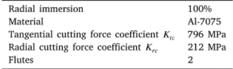
Table 2

Machining parameters used to predicted stability lobes forFig. 3(d–f)

Radial immersion 100%

Material Al-7075

Tangential cutting force coefficient�� 796 MPa

Radial cutting force coefficient�� 212 MPa

Flutes 2

In previous work, Erturk et al. [31] demonstrated the effect of changes in the tool holder diameter through simulations, conducting a sensitivity analysis for two scenarios. The first case was when all the diameters in the tool holder were increased by 10 mm, and the second case was when the middle diameter was increased by 40 mm. However, to the authors’ knowledge, there exists no experimental data set that demonstrates the effect of this geometry on the tool-tip frequency response function and, therefore, on the stability of a milling operation. Therefore, this section will present the results of an experimental investigation into the potential of the tool-holder geometry to influence chatter stability boundaries.

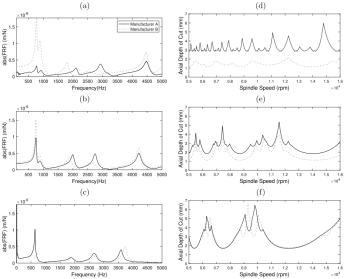
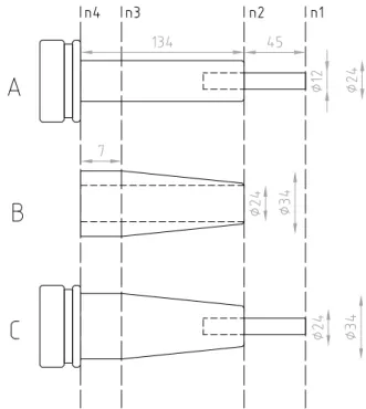
Six HSK63 shrink fit tool holders were tested, from two manufactur-ers and each using three tool diametmanufactur-ers. The geometries of each of the tool-holders and solid carbide end-mills are given inFig. 2andTable 1. It can be seen that the tool-holders differ only by their base diameter�2. Also, as the tool diameter increases the difference in geometry between the two holders decreases. The base diameter of the 12 mm tool-holders differs by 19 mm, whilst the 25 mm tool-tool-holders differ by just 0.5 mm.

In order to observe the effect of the various geometries, tools were inserted into each of the tool-holders, with identical stickout lengths, and the tool tip frequency response function measured when mounted on a Starrag ZT-1000 5 axis milling centre. In each test, a Bilz

(6)

Fig. 3.FRFs (a–c) and Stability lobe diagrams (e–f) comparing tool-holders from manufacturer A and B, for the 12 mm (a, d), 16 mm (b, e), and 25 mm (c, f) diameter tools. ThermoGrip inductive shrink unit with water cooling was used to

mount the tool in the holder, with accurate control of the stickout length. Impact tests were then carried out using a PCB Piezotronics modally tuned impulse hammer (model 086C01). The response was measured at the tool tip using a PCB Piezotronics ceramic accelerome-ter (model 352C23) and 10 averages were taken for each test. Analysis and stability prediction was performed using the Metal Max DT9837 data acquisition (DAQ) board, and the Metal Max software. The results are compared in Fig. 3(a–c), along with the corresponding stability lobe diagrams (Fig. 3(d–f)) based on the machining parameters listed inTable 2.

With reference toFig. 3(a–c) the actual dynamic properties of the tool-holders are not important here, but the overall trend as their geometries converge is of particular note. The two 12 mm tool-holders produce significantly different tool tip dynamics, with the amplitude of the most dominant mode for manufacturer B around three times larger than that of manufacturer A. Moreover, the modes between 1500 Hz and 3500 Hz see a considerable reduction in natural frequency as the base diameter is increased. As the difference in the tool-holder geom-etry reduces, the difference between the tool tip FRFs also diminishes. The 25 mm tool-holders, which have almost identical base diameters, produce extremely similar results.

The stability of these six configurations can be seen in Fig. 3(d– f). These assumed that the (arbitrary) machining parameters listed if Table 2 were used. For the 12 mm tool-holders (Fig. 3(d)), the increased base diameter of manufacturer A produces a substantially larger absolute stability limit. The effect on the lobe location is perhaps again more complex. The most dominant mode for manufacturer A is

at around 3000 Hz (Fig. 3(a)), much higher than that of manufacturer B at around 750 Hz. This results in more closely spaced lobes. Once again, as the geometry of the tool-holders converges so to does their stability.Fig. 3(e) and3(f) compare the stability of the 16 mm and 25 mm tool-holders respectively. It can be seen that both the absolute stability limit and lobe location converge with base diameter.

One observation from these results is that the larger base diame-ter tool holder achieves a stiffer structure which thereby ensures an increase in the limiting critical depth of cut - a valuable and well-known concept. However, the aim of the current study is to investigate how the geometry of the tool holder can be used to fine tune the dynamics of the structure and thereby adjust the stability lobes in order to achieve satisfactory performance at a particular spindle speed. There have been various studies [12–14] that have explored this concept from the perspective of the tool (e.g. tool stickout length), but to the authors’ knowledge the tool holder itself has been overlooked.

As an aside, the FRF experiments and stability predictions were repeated on a second machining centre, a Cincinnati FTV5. Despite the difference in spindle (machine) dynamics, the trend in the results corresponded to that of the Starrag ZT-1000, and so the results are not included here for conciseness.

3.1. Summary

It has been shown, for the first time in published literature, that the tool-holder base diameter has a significant effect on the tool tip dynamics and, in turn, on the stability of a milling operation. It is

(7)

therefore proposed that, the base diameter may be tuned in order to optimise the stability threshold for a given operation. Whilst it has been shown previously that the tool stickout length provides similar optimisation capability, the practical application of this is plagued by the requirement to measure or model the changing interface dynamics between the tool and tool-holder. It will now be shown that by using structural modification with the tool-holder base diameter as the tuning parameter, this requirement can be removed.

4. Structural modification for the selection of an optimal tool-holder

Since the geometry, and more specifically the diameter, of the tool-holder has a significant effect on the tool tip dynamics, and in turn the stability of the milling operation, a simple method of avoiding chatter, whilst maximising the material removal rate, would be to select a tool-holder diameter that results in stability lobes at an optimal spindle speed [32]. Whilst it is perfectly reasonable to suggest that the RCSA method be used to streamline this process by predicting the dynamics of each available tool-holder from a single experimental model, the method suffers from two drawbacks. Firstly, the accuracy of the result is dependent on knowledge of the interface dynamics between the tool and tool-holder. Secondly, the optimal tool-holder geometry must be found indirectly by repeating the process for every available tool-holder. It will now be shown how structural modification can be used to avoid these difficulties.

The application of structural modification for tool-holder optimisa-tion is presented in three secoptimisa-tions. Firstly, the methodology is intro-duced which describes how each of the models necessary for structural modification are constructed. Secondly, the Direct Structural Modifi-cation method is used to predict the tool tip FRF when changes are made to the tool-holder diameter. This matches the capability of the RCSA method, whilst removing the requirement for knowledge of the interface dynamics. Lastly, the Inverse Structural Modification method is used to predict what diameter tool-holder is needed to produce a natural frequency (and therefore a peak in the SLD) at the required location. This extends the capability of RCSA by allowing the optimal tool-holder diameter to be found by solving a single simple equation whilst also removing the requirement for knowledge of the interface dynamics.

4.1. Methodology

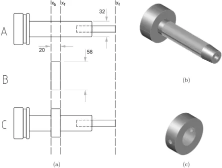
This section describes how each of the models (�and�), defined in Eq.(2)and applied in Eqs.(8)and(9)are constructed. The geometry of these models is seen in Fig. 4. In order to investigate structural modification for chatter avoidance in high speed milling, two tool-holders of different geometries were chosen. A cylindrical untapered tool-holder of length 0.134 m and diameter 0.024 m; and a tapered tool-holder of length 0.134 m and diameter ranging between 0.024 m and 0.034 m. These tool-holders will be referred to as the unmodified (model�) and modified (model�) tool-holders respectively.

4.1.1. Model�

It is convenient to begin the methodology by discussing model�,

or the modification model, which is a numerical model that describes the difference in diameter between the unmodified and modified tool-holders. The geometry is a circular tube of length 0.134 m with an inner diameter of 0.024 m. The outer diameter varies between 0.024 m and 0.034 m, as shown inFig. 4. A numerical model was constructed with the geometrical properties shown, and standard steel material properties (density�= 7750kg m−3, Young’s Modulus�= 200 GPa).

The geometry of model � was modelled using only two beam

elements, one for the tapered section of the tool-holder and one for the untapered section. The first beam lies between nodes�₂and�₃and the second between nodes �3and�4, as shown inFig. 4. Each beam

Fig. 4. Diagram detailing the location of the nodes included in models A B C.

has two degrees of freedom, translation� and rotation�. Therefore, the dimensions of the elemental matrices are 6×6.

Beam one (between �2 and �3) is a tapered Timoshenko tube,

constructed from the beam element matrices given in [33], it has an inner diameter of 0.024 m, an outer diameter between 0.024 m and 0.034 m, and a length of 0.127 m. Whilst the second beam is an un-tapered Timoshenko tube, constructed from the standard Timoshenko beam element matrices [34], with an inner diameter of 0.024 m, an outer diameter of 0.034 m, and a length of 0.07 m. Timoshenko beam elements were used over Euler–Bernoulli beam elements, since it has already been shown that they describe the dynamics of tool-holders with greater accuracy [35].

The global mass and stiffness matrices for model�were then

assem-bled using the direct stiffness method, which applies compatibility and equilibrium conditions in a similar manner to structural modification. The global mass and stiffness matrices are then given by

�₌ ⎡ ⎢ ⎢ ⎣ [ � 22 ] 2×2 [ � 23 ] 2×2 � [ � 32 ] 2×2 [ � 33 ] 2×2 [ � 34 ] 2×2 � [� 43 ] 2×2 [ � 44 ] 2×2 ⎤ ⎥ ⎥ ⎦ (10) and �₌ ⎡ ⎢ ⎢ ⎣ [ � 22 ] 2×2 [ � 23 ] 2×2 � [ � 32 ] 2×2 [ � 33 ] 2×2 [ � 34 ] 2×2 � [� 43 ] 2×2 [ � 44 ] 2×2 ⎤ ⎥ ⎥ ⎦ (11) respectively, where the subscripts�� refer to the nodes�2-�4, and�

�� and�

�� are given in(A.3). Then finally, for a particular frequency� model�is given by:

�

� �=�+��−�2�

=(1 +��_�)�_{+ (}��_�−�2)�

where�_�and�_�are the proportional damping coefficients found from

the experimental modal [8] model and defined in(A.1).

4.1.2. Model�

To construct model�, the experimental translational mode shapes �_�were measured at 18 equally spaced locations between the tool tip

(8)

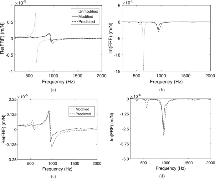
Fig. 5. Real (a) and Imaginary (b) frequency response function plots comparing the experimental tool tip dynamics of the modified (—) tool-holder, with the results of the Direct Structural Modification in the�-direction (- -) on the FTV5. [c] and (d) show close-ups of the predicted and experimental modified tool holder.

In total 8 modes were extracted from the raw FRF data with natural frequencies between 273 Hz to 4045 Hz. Then to each of the eight modes a polynomial of order three was fitted in the least-squares sense. Each of the eight polynomials were then differentiated to get the rota-tional mode shapes�(1)_� . Whilst the rotational information can be found

by differentiating the translational FRFs directly, modal differentiation consistently produced more accurate results. Then for each of the four nodes�1to�4shown inFig. 4, the translational and rotational FRFs (�_��, �_��, �_��, �_��) with �, � ∈ {1,2,3,4} were constructed using Eq.(A.5). The accuracy of this method depends largely on the number of data points included in the polynomial fitting. Increasing the number of data points was found to increase the accuracy of the rotational mode shapes, whilst decreasing the efficiency of the method. It was found that using eighteen data points continuously produced accurate results for all modes, although it was not always necessary.

Model �was then constructed, for a particular frequency �, as follows � �= [[ � �� ] 2×2 [ � �� ] 2×6 [ � ��  ] 6×2 [ � ��  ] 6×6 ] = ⎡ ⎢ ⎢ ⎢ ⎢ ⎣ [ � 11 ] 2×2 [ � 12 ] 2×2 [ � 13 ] 2×2 [ � 14 ] 2×2 [ � 21 ] 2×2 [ � 22 ] 2×2 [ � 23 ] 2×2 [ � 24 ] 2×2 [ � 31 ] 2×2 [ � 32 ] 2×2 [ � 33 ] 2×2 [ � 34 ] 2×2 [ � 41 ] 2×2 [ � 42 ] 2×2 [ � 43 ] 2×2 [ � 44 ] 2×2 ⎤ ⎥ ⎥ ⎥ ⎥ ⎦

where the subscripts 1–4 refer to the nodes�1-�4, and [ � �� ] 2×2= [ �_��(�) �_��(�) �_��(�) �_��(�) ] (12)

4.2. Direct structural modification

Using the models constructed in section. 4.1, the Direct Struc-tural Modification method was carried out by applying Eq.(8)over a frequency range of 1 Hz–5000 Hz with a 1 Hz increment. The resultant matrix (for each frequency) �

��  contains the four FRFs (�_�11, �_�11, �_�11, �_�11), from which the translational tool tip FRF �_�11was extracted.

The practical implementation of structural modification approaches requires experimental measurements of the frequency response func-tion at the interface between the modelled and physical components. With reference toFig. 4, for the current approach this requires measure-ments at the tool tip (n1), the start and end of the tool holder (n2, n4) as well as the location of a change in geometry within the toolholder (n3). Furthermore, as with any structural modification method, rota-tional FRFs must be estimated at these locations. In the present study, these measurements were obtained by performing a range of frequency response function tests along the length of the tool holder and tool. Then, a modal model was obtained and a 3rd order polynomial fitted to this in order to obtain an empirical analytical expression for the mode shapes and their derivatives. Although this approach requires more

(9)

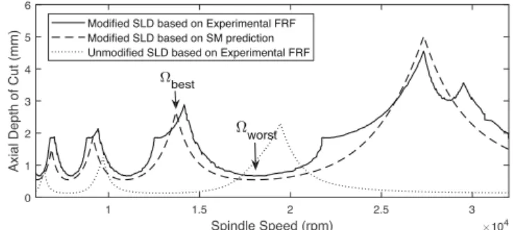
Fig. 6. Stability lobe diagrams for the modified tool-holder on the FTV5 (experimental (—) vs. predicted (- -)).

experimental data than alternatives, it is a robust means of obtaining rotational frequency response functions and enabling a diverse range of modifications to be explored (such as complex changes in geometry) without having to gather additional experimental data.

An alternative approach to this would be to measure the rotational frequency response functions using a finite difference method [29] in order to approximate the rotational information. However, the ac-curacy of this method is limited by the user’s choice of the spacing between translational measurements. Gibbons et al. [30] have pre-sented an optimised finite difference method for beam-like structures, such as tools and tool-holders, which can improve the accuracy of this method.

The results of the Direct Structural Modification method in the�

direction on the FTV5 are plotted inFig. 5, along with the measured tool tip FRFs for the unmodified and modified tool-holders. It is clear to see that the predicted and measured tool tip FRFs for the modified tool-holder are highly correlated. The purpose of this experiment is to predict the stability of a milling operation; therefore, a stability lobe diagram was generated from both the measured and predicted tool tip FRFs. The assumed machining parameters are shown inTable 2. The results are compared inFig. 6. It can be seen that the Direct method very accurately predicts the absolute stability limit at�_worst, which is

determined by the minimum of the real part of the oriented FRF; as well as the location of �_best, determined by the natural frequency of

the oriented FRF. There is however some error in the gradient of the stability limit between�_worstand the next peak, this is determined by

the rate at which the real part of the FRF returns to zero following a mode.

There are three possible reasons for the difference between the two predictions. First, the approach to obtaining experimental frequency response functions has involved the construction of a modal model from experimental data. If this model neglects some modes from the original structure, then the prediction will not include these modes. Second, the original structure could include symmetric modes which are not fully identified by the modal model. When the modification is added to the structure, the symmetry of the modes could be broken, which again results in un-modelled modes that are neglected in the predic-tions. Third, the modification involves an assumption of proportional damping, which may not reflect the physical behaviour of the system.

When compared to the RCSA method, the Direct Structural Modi-fication method has a simple advantage, in that only a single experi-mental model from a standard tool-holder is required, and no further measurements or models (such as interface parameters) are needed. The disadvantage over RCSA is the size of the numerical model. In this application 18 FRFs were measured and whilst this may not always be necessary, it is significantly more than standard 3 FRFs required to apply RCSA. It should also be noted that model�was constructed

using the minimum number of elements required, and results could be improved by using a larger number. The advantage of this must be weighed up against the increased experimental cost, as more nodes in model B would require more experimental nodes in model�.

Whilst this method has clear advantages over previously proposed methods, the optimisation process still requires the construction of several analytical models (one for each tool-holder available), which could easily become a lengthy process. Therefore, in the next section, it will be shown how the Inverse Structural Modification method can be used to select the optimal tool-holder with a single analytical model by solving a single simple equation.

4.3. Inverse structural modification

The advantage of Inverse Structural Modification method over the direct method is that an optimal tool-holder geometry can be selected by solving a single simple equation. This involves building a single partially constructed numerical model and is thus computationally far less expensive than the direct method.

To apply Inverse Structural Modification to the same example as above, model �was constructed using the same methodology as in

Section 4.1.2. Then, the same beam elements as before were used to construct model�; however, a symbolic variable�2was used for the outer diameter of the beams instead of inputting an actual value. Therefore, the tapered beam has an inner diameter of 0.024 m and an outer diameter ranging between 0.024 m and�2, and the untapered beam has an inner diameter of 0.024 m and an outer diameter of�2.

In doing so, model�becomes a symbolic matrix and a function of�2.

Since the dominant natural frequency of the modified tool-holder occurs at 936 Hz, Inverse Structural Modification was used to seek a value of�2which would result in a mode at 936 Hz, therefore�_��= 2�(936) rad/s. Referring back to Eq.(9), the natural frequencies of the

modified model�are given by

det(�₊�

�� �� �(�2)) = 0 (13)

To solve this, the matrix�

�� is given by � �� = ⎡ ⎢ ⎢ ⎣ [_� 22(��) ] 2×2 [_� 23(��) ] 2×2 [_� 24(��) ] 2×2 [ � 32(��) ] 2×2 [ � 33(��) ] 2×2 [ � 34(��) ] 2×2 [ � 42(��) ] 2×2 [ � 43(��) ] 2×2 [ � 44(��) ] 2×2 ⎤ ⎥ ⎥ ⎦ (14) Since damping has no effect on the natural frequencies of a structure, model�is given by

�

� �(�2) =�(�2) −�2��(�2) (15) Then, evaluating Eq.(15)results in a polynomial in�2of order 36, with complex coefficients. Since�2is real, the real and imaginary parts of the polynomial are set to zero and solved individually. The polynomials are too large to solve analytically, however using Newton’s method to find the roots of the polynomial, a numerical solution was found, giving 36 possible diameters. However, some of these solutions can be instantly disregarded, firstly all negative solutions were removed, and then solutions outside of the possible range for�2were also discounted. Since the base diameter�2cannot exceed the flange diameter�1, it has

an allowable range of0 ∶ 024< �2<0 ∶ 064m. This resulted in a single solution of 0.0336 m. It is already known that a diameter of 0.034 m results in a mode at 936 Hz, hence the solution is correct to within 0.0004 mm. Therefore, it has been shown that the Inverse method may be used to select an optimal tool-holder geometry by solving a simple equation with a single partially constructed analytical model, a feature that is not present in the RCSA method.

4.4. Summary

Both the Direct and Inverse Structural Modification methods have been applied to the chatter avoidance problem. The Direct method provides a novel means of modelling how changes in the tool-holder ge-ometry effect the tool tip dynamics, and thus the stability of the milling operation. This matches the capability of RCSA, whilst removing the requirement for knowledge of the interface dynamics. In order to streamline the optimisation process, the Inverse Structural Modification

(10)

method was also introduced. This method allows the user to predict a tool-holder diameter that will result in a stable peak in the stability threshold at the required spindle speed. This extends the capability of RCSA by not only removing the requirement for knowledge of the interface but by also limiting the required number of numerical models to one.

5. A new tunable-mass tool-holder

The previous section demonstrated how structural modification may be used to model the geometry of a standard tapered tool-holder in an attempt to optimise the stability threshold of a milling operation. Consequently, the optimal tool-holder may be selected from the range available in order to avoid chatter whilst maximising material removal rates. However, the method shown relies on the user having a large range of tool-holders, with a range of geometries, from which to choose and there is no guarantee that the optimal geometry will be available. This can lead to a significant financial investment from the manufacturer. The purpose of this section is to outline the design and testing of a new tunable-mass tool-holder, which allows the user to tune the dynamics of the machine in order to optimise the stability threshold using a single tool-holder. Thus streamlining the optimisation process and reducing the cost for the user.

This section is presented as follows. Firstly, the design of the tunable-mass tool-holder is presented and its functionality explained. Secondly, the dynamic performance of the tool-holder in a range of configurations is presented to demonstrate its capability. Lastly, the cutting performance of the tool-holder is presented with the results of a set of cutting trials. Throughout, the Direct Structural Modification method is used to model changes in the geometry of the tunable-mass tool-holder.

5.1. Design solution

The design for the tunable shrink-fit tool-holder is pictured in Fig. 7. Model �shows the tunable-mass tool-holder which consists

of the standard HSKA63 interface, a threaded tool-holder shaft, and tool clamping capabilities. The collar is a simple cylindrical component with radial grub screws, and the tool holder is modified so that it is a shaft with sufficient material to maintain the structural integrity of the shrink-fit interface . A threaded interface on the tool-holder allows the collar (model�), to be moved up and down the length of the

tool-holder. Running along the side of the tool-holder shaft are two parallel flat surfaces, which are used to secure the collar in place. As the collar is rotated up and down the tool-holder, a grub screw can be passed through the two parallel threaded holes in the wall of the collar, the grub screws then attach on to the level surfaces and hold the collar in place. With this design, it is straightforward to add the collar and adjust its position after an endmill has been shrunk-fit into the holder. In its simplest form this design does mean that the tool holder must have a constant diameter along the threaded region (as shown inFig. 7b), although more intricate designs could avoid this constraint by using alternative mechanical assemblies.

5.2. The dynamic performance of the tunable-mass tool-holder

A series of laboratory experiments were performed to test the dynamic performance of the tunable-mass tool-holder and verify that the Direct Structural Modification method is capable of predicting the dynamic behaviour of the tool-holder. If these assumptions hold, then the tunable-mass tool-holder may be used to shift the stable peaks in the stability threshold, and the Direct Structural Modification method can be used to find the optimum collar location, without having to perform multiple experimental modal analyses.

To begin, experiments were performed on a specially designed spindle rig in order to validate the theoretical approach in a laboratory environment . The rig consists of a HSK milling spindle (model GMN

HV-P 150y - 30000/26 HSK-C63 R), including bearings and bearing housing, similar to any five axis milling machine, but is suspended on a smaller simpler structure. A standard 12 mm two flute milling tool was inserted into the tool-holder with a stickout length of 40 mm.

Initially, in order to test the dynamic performance of the tool-holder the tool-tip FRF with the collar at the base of the tool-holder was measured, then the collar was gradually moved along the shaft of the tool-holder towards the tip, measuring the tool-tip FRF at 6 linearly spaced locations along the shaft.

Then, the Direct Structural Modification method was used to predict the tool-tip FRF of the tool-holder with the collar in the same 6 locations. In this application of the method, model � contained an

experimental model of the tunable-mass tool-holder with no collar, and model�was an analytical model of the collar.

To construct model�, the translational and rotational mode shapes of the tool-holder with no collar were measured as in Section4.1.2. The model consists of three nodes (as seen inFig. 7),�_�, the tool tip, �_�, where the front of the collar will be, and�_�, where the back of the collar will be, each of which has two degrees of freedom, translation�

and rotation�. Then at a particular frequency model�is constructed

as � �= [ [� ��]2×2 [���]2×4 [� �� ]4×2 [��� ]4×4 ] = ⎡ ⎢ ⎢ ⎣ [� ��]2×2 [��]2×2 [��]2×2 [� � �]2×2 [�� �]2×2 [�� �]2×2 [� ��]2×2 [��]2×2 [��]2×2 ⎤ ⎥ ⎥ ⎦ (16)

where the subscripts�,�and�refer to the nodes�_�,�_�and�_�and�

�� is given in Eq.(12).

The numerical model�, which describes the dynamics of the collar itself, is simply an untapered Timoshenko tube, constructed from the elemental matrices (�and�) in [34]. Proportional damping was again

included in the model using the experimental modal model from model

�. Since the collar is not rigidly attached to the tool-holder, it has no effect on the stiffness of the overall structure [8], therefore stiffness was not included in the numerical model, and hence only the mass and damping are modified. Therefore, for a particular frequency�, model �is given by

�

� �=��−�2�

= (��_��)�_{+ (}��_��−�2)�

where�_�and�_�are the proportional damping coefficients found from the experimental modal model [8], and

�₌ [[ � � � ] 2×2 [ � � � ] 2×2 [ � �� ] 2×2 [ � �� ] 2×2 ] and �₌ [[ � � � ] 2×2 [ � � � ] 2×2 [ � �� ] 2×2 [ � �� ] 2×2 ] (17) where �

�� and �� are given in (A.3). Then the Direct Structural Modification method was applied using the Eq.(8)and the tool-tip FRF extracted. This was repeated for each of the 6 collar locations.

The results of the experiments are presented inFig. 8which presents the experimental tool-tip FRFs of the tool-holder with no collar and with the collar in the 6 linearly spaced locations, along with the 6 predictions of the Direct Structural Modification method. With the addition of the collar, a reasonably small decrease in the dominant natural frequency of 16 Hz is seen. Then, the natural frequency de-creases linearly with the distance from the flange of the tool-holder. With the collar at 54 mm, a total shift of 52 Hz occurs, which for a tool with two flutes, would results in a shift of 1560 rpm in the first stability lobe. However, there is also the potential to move this collar further, and hence the potential for larger frequency shifts. It can also be seen that the predictions of the Direct Structural Modification method are highly correlated to the measured FRFs. Therefore, it can be concluded that the tunable-mass tool-holder is capable of producing a significant shift in the stable peaks of the stability threshold. More-over, the Direct Structural Modification method can accurately predict

(11)

Fig. 7.The design solution for a mass-tuned tool-holder. (a) Engineering drawing with collar dimensions in mm; (b) tunable tool holder 3D view; (c) adjustable collar 3D view.

Fig. 8. Experimental tool tip FRFs (Real and Imaginary parts) of the prototype with no collar (…) and with collar C1 (—) compared with the Direct Structural Modification prediction (- -). From right to left the collar is positioned at4,14,24,34,44,54mm from the flange of the tool-holder.

the dynamics, and therefore stability, of the tunable-mass tool-holder and can consequently be used to optimise the stability of a milling operation.

The curve fitting method for rotational degree-of-freedom synthesis has a particular advantage when using the prototype in that a full modal model is constructed, from which FRFs at any location along the length of the tool/tool-holder can be extracted i.e. the mode shapes are continuous in the spatial coordinate. Since the location of the collar (�_� and�_�) is variable, it is possible to apply the Direct Structural

Modification method with the collar in any location using a single experimental model. Therefore, it is not necessary to know the location or length of the collar before measuring the modal model. In practice, a range of collars of various length and diameter could be designed to maximise the tunability of the tool-holder.

5.3. The cutting performance of the tunable-mass tool-holder

Now that the tunable-mass tool-holder and Direct Structural Modifi-cation method have been experimentally validated on a spindle rig, this

section will firstly show that similar results may also be achieved from an industrial standard milling machine. For the tool-holder to have a significant financial benefit to the manufacturing industry, the user must be able to predict stable cutting parameters from the predicted stability lobe diagram. Therefore, secondly, this section will focus on the cutting performance of the tool-holder. Results of a milling trial are used to determine the experimental stability of the prototype in its various configurations. These experimental results are then compared to their predicted counterparts, calculated using the Direct Structural Modification method.

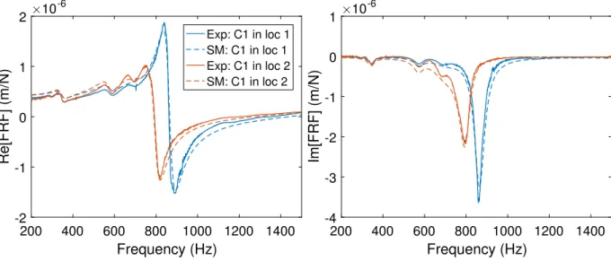
The results of the Direct Structural Modification method applied on the FTV5 milling machine are presented inFig. 9. The results show the predicted tool-tip FRF for the tool-holder in 2 different configurations; with the collar in location 1, where the back of the collar is measured at 4 mm from the flange, and location 2 at 64 mm. These predictions are also compared with their experimental counterparts.Fig. 9shows the Direct Structural Modification method accurately predicts the modes of the tunable-mass tool-holder in both configurations. Therefore, it can be concluded that the Direct Structural Modification method is sufficiently accurate for use on an industry standard milling machine.

(12)

Fig. 9. Real and imaginary parts of the tool tip FRF for the prototype with the collar 4 mm from flange (measured (—) and predicted (- -)) and collar C1 64 mm from flange (measured (—) and predicted (- -)). (For interpretation of the references to colour in this figure legend, the reader is referred to the web version of this article.)

Table 3

Machining parameters used to predicted stability lobes forFig. 11(a–b)

Parameter Value Radial immersion 50% Material Al-6082 �� 614.14 MPa �� −15.48 MPa Flutes 2

ComparingFig. 8with9, it can be seen that the tunable tool holder can achieve a similar performance in both the laboratory and industrial environment, with a shift in the dominant natural frequency of over 50 Hz in both cases.

The SLDs for the tunable-mass tool-holder were now calculated [36] for the chosen machining parameters listed in Table 3. In order to validate these stability predictions a number of milling operation were performed over a range of spindle speeds and depths of cut. Each setup was tested in turn, cutting at spindle speeds of between 5000 rpm and 15 000 rpm. The speeds and depths were chosen based on the individual stability lobe diagrams, so as to accurately capture the characteristics of each in enough detail to validate the prediction. A milling operation with half radial immersion (6 mm) and feed per tooth of 0.05 mm/tooth was chosen based on the recommendations of the tool manufacturer.

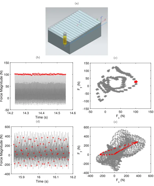
For each combination of speed and depth the stability was de-termined by monitoring force and sound signals recorded during the cut. Each test configuration involved machining of a stepped work-piece with 0.5 mm increments in the depth of cut, from 1 mm to 10 mm. The workpiece was mounted on a Kistler 9255B large plate dynamometer and audio recordings made via the CutPro MALDaq interface. Classification of chatter was made using a combination of three methods:

•Visual inspection of the finished surface

•Once per revolution sampling was used to obtain Poincaré sec-tions of the dynamometer signals [37]

•Frequency domain analysis of the sound spectrum obtained from the audio recording [38].

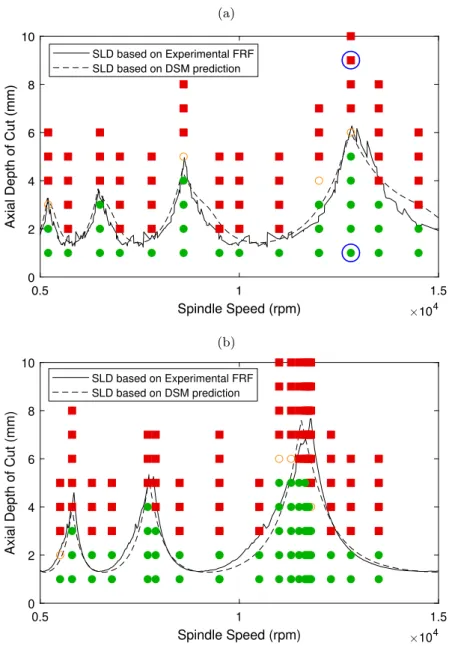
Examples of the machining trials and the Poincaré analysis are shown in Fig. 10. Full details of the cutting trial can be found in [8]. The results are summarised inFig. 11. The Direct Structural Mod-ification prediction for the collar in location 1 (Fig. 11(a)) shows high correlation with both the experimental stability lobe diagram as well as the experimental stability points, determined by the force

and sound signals. Each of the four lobes predicted by the Direct Structural Modification method also occur in the experimental data, and the absolute stability limit matches that of the force and sound data. Fig. 11(b) shows the results for the collar in location 2, and demonstrates similar accuracy to that of the first configuration. In this case, the three lobes are predicted at the correct spindle speed and the stability limit complements the experimental data. Comparing the two diagrams, a significant shift in the lobes can be seen. The accuracy of the results, as well as the shift in the lobes, draw the conclusion that the tunable-mass tool-holder may be used to tune the dynamics of a milling machine, and thus optimise the stability threshold for a given operation.

InFig. 12, the stability lobes fromFig. 11are shown superimposed. It can be seen that the change in position of the collar can have a significant impact on the stability lobes. Whilst it is also apparent that the ‘no collar’ stability lobe is similar to that with the collar at its base position, it is also the case that this performance is accurately predicted by the theory. Furthermore, it is not surprising that the collar has a limited impact when it is located here, because the additional mass and stiffness is small compared to that of the adjacent flange.

5.4. Summary

The design for a new tunable-mass tool-holder has been presented. The tool-holder allows the user to tune the dynamics of the machine in order to optimise the stability threshold of a milling operation, without the need to purchase a wide range of tool-holders. The dynamic performance of the new tool-holder has been presented on both a spindle rig and an industry standard milling machine and, it has been shown that the Direct Structural Modification method can be used to model changes in the tool-holder’s configuration. Moreover, the cutting performance of the new tool-holder has been experimentally verified via a set of milling trials.

6. Discussion

A number of aspects are worthy of further discussion.

6.1. Interface dynamics

One benefit of the proposed approach, when compared to alterna-tive applications in machining dynamics, is that the prediction accuracy is less sensitive to the dynamics of the interface between machine

(13)

Fig. 10. Machining trials, with examples of stable and unstable cutting forces with the collar at location one. (a) workpiece configuration; (b), (d): Time history of�-direction forces; (c), (e):�-vs.�-direction forces. Once per revolution sampled data is shown by+markers. At 1 mm, 12800 rpm ((b), (c)) the response is stable with a low variance in the once-per-revolution samples. At 9 mm, 12800 rpm ((d), (e)), the response is unstable with a high variance in the once-per-revolution samples, and quasi-periodic motion that indicates a secondary Hopf bifurcation.

elements. For example, when structural modification concepts are used to predict the influence of a change in the tool geometry, the approach requires an accurate model of the interface between the tool and tool holder [15,16], and this behaviour may be difficult to model. In contrast, with the theory used in this work real-world tool to toolholder interface is part of the physical model (model A), and is therefore based directly upon experimental data. For the tunable tool-holder, a new physical interface is created between the main tool holder and the additional collar. This is an additional machine element contact, but it does not lie across the full load path from tool to spindle, thus reducing the model’s sensitivity to interface dynamics. However, for a non-tuned tool holder (e.g. designed using the inverse method, Section4.3), the resulting tool holder is a monolithic structure which completely eliminates the problem of modelling real-world interface dynamics.

6.2. Practical considerations

6.2.1. Using the direct method in industrial practice

The direct method (Section4.2) has been rigorously validated in the previous sections. From an industrial perspective, the approach can be used to tune a toolholder in a variety of ways. Perhaps the simplest approach would be to confirm which tool holder (from an existing inventory) is most appropriate for a particular machining scenario. To achieve this, the inventory of tool holders needs to be complemented by: (a) a single experimental data set for a baseline toolholder that defines Model A (Fig. 4) for the machine and tool under consideration; (b) a set of numerical models that define the different toolholder geometries (Model B). With this approach, only one toolholder needs to be tested experimentally (the baseline toolholder), and from this the

(14)

Fig. 11. Experimentally validated stability lobe diagrams for prototype with collar in: (a) location one, 4 mm from the flange, (b) location two, 64 mm from the flange. Red squares show unstable machining tests, green circles show stable machining tests, and hollow orange circles show marginally stable machining tests. Blue circles indicate the two tests illustrated inFig. 10. (For interpretation of the references to colour in this figure legend, the reader is referred to the web version of this article.)

performance of all other toolholders can be explored through stability lobe predictions similar to those shown inFig. 12.

Alternatively, the direct method can be used to retune a tunable toolholder, as described in Section 5. This can involve changes in the collar position, or other geometrical changes such as the collar length or diameter. Again, the implementation would require a single experimental data set for a baseline toolholder that defines Model A, and would lead to a prediction of stability scenarios as shown inFig. 12.

6.2.2. Using the inverse method in industrial practice

The inverse method (Section 4.3) relies on the same theoretical approach as the direct method, but it enables an analytical solution to the geometrical configuration of the tool holder, based upon a target spindle speed. In practice this is likely to be of value for high volume production scenarios where a specific spindle speed is demanded as part of the process specification. In this case, the method enables the design of a bespoke tool holder with stability lobes tuned to meet the requirements, by adjusting the diameter of the tool holder base. To achieve this, an initial tool holder design should be tested with an impact hammer in order to generate model A (Fig. 4). Then, the theory

allows for an optimised design of model C, by analytically adjusting the geometry shown in Model B. One advantage of this approach is that experimental frequency response measurements are only required at the specific node points shown inFig. 4. The final tool holder can be chosen by either: selecting from a suite of tool holder to fit the required base diameter; custom manufacturing a tool holder to meet the requirements; or using a tunable tool holder with a different collar diameter.

Whilst the inverse method has not been experimentally applied here, it relies on the same theory as the Direct Method, and so further validation is not necessary. However, further work could explore the simultaneous optimisation of multiple design parameters, such as the collar diameter, length and collar location.

6.2.3. Impact of tool diameter

One issue that merits further discussion is the utility of the proposed approach on different diameters of tool. It is well known that for small tool diameters the structural dynamics tend to be more influenced by the tool modes of vibration, where the tool behaves like a simple can-tilever. Meanwhile, for larger diameter tools the opposite happens, and

(15)

Fig. 12. Comparison of stability lobes with no collar (blue lines), collar at location one (green lines), collar at location two (red lines). Predicted stability lobes, based upon the direct structural modification method, are shown as dashed lines. There is no prediction required for the case with no collar. (For interpretation of the references to colour in this figure legend, the reader is referred to the web version of this article.)

Fig. 13. Mode shapes (first six modes) for the tunable tool holder with no collar attached. (a) mounted on the spindle rig; (b) mounted on the FTV5 machine. the structural dynamics become dominated by the modes of vibration

of the spindle, toolholder, and machine structure.

In the present study, a relatively low diameter tool (12 mm diameter tool with 40 mm stickout length) was chosen for the mass-tuned tool holder, and the resulting mode shapes when mounted on the spindle test rig and the FTV5 machine are illustrated inFig. 13. Compared to larger diameter tools, the tool modes are relatively important in the overall response shown in13, whereas for smaller diameter tools the tool mode is more likely to dominate. In practice, this variation could have an impact on the ability of the tool holder to influence the stability lobes.

Despite this, the tunable tool holder has been shown to achieve good performance in terms of its ability to adjust the dynamics of the structure and thereby optimise the stability lobe locations.

6.2.4. Relevance to five axis machining

A final consideration for the use of the tunable tool holder is the case of complex five axis machining operations, where the geometry of the tool holder might be more heavily constrained by the production process. An example might be aero-engine blisk machining. It is true that due to the additional collar on the tool holder, there are additional collision risks with the workpiece. However, this risk can be mitigated by offline simulation of the toolpaths using NC verification software and, if needed, rotational degrees of freedom, namely, lead and tilt angles may need to be adjusted.

7. Conclusion

This paper has presented a novel application of structural modi-fication theory to the chatter avoidance problem. A new dataset has been presented which shows the potential influence that tool-holder