BIPEDAL WALKING ANALYSIS, CONTROL, AND APPLICATIONS TOWARDS HUMAN-LIKE BEHAVIOR
A Dissertation by
KENNETH YI-WEN CHAO
Submitted to the Office of Graduate and Professional Studies of Texas A&M University
in partial fulfillment of the requirements for the degree of DOCTOR OF PHILOSOPHY
Chair of Committee, Pilwon Hur Committee Members, John Buchanan
Prabhakar Pagilla Sivakumar Rathinam Head of Department, Andreas Polycarpou
May 2019
Major Subject: Mechanical Engineering
ABSTRACT
Realizing the essentials of bipedal walking balance is one of the core studies in both robotics and biomechanics. Although the recent developments of walking control on bipedal robots have brought the humanoid automation to a different level, the walking performance is still limited compared to human walking, which also restricts the related applications in biomechanics and rehabilitation.
To mitigate the discrepancy between robotic walking and human walking, this disser-tation is broken into three parts to develop the control methods to improve three important perspectives: predictive walking behavior, gait optimization, and stepping strategy. To improve the predictive walking behavior captured by the model predictive control (MPC) which is transitionally applied with the nonlinear tracking control in sequence, a quadratic program (QP)-based controller is proposed to unify center of mass (COM) planning using MPC and a nonlinear torque control with control Lyapunov function (CLF). For the gait optimization, we focus on the algorithms of trajectory optimization with direct colloca-tion framework. We propose a robust trajectory optimizacolloca-tion using step-time sampling for a simple walker under terrain uncertainties. Towards generating human-like walking gait with multi-domain (phases), we improve the optimization through contact with more accurate transcription method for level walking, and generalize the hybrid zero dynamics (HZD) gait optimization with modified contact conditions for walking on various terrains. The results are compared with human walking gaits, where the similar trends and the sources of discrepancies are identified. In the third part for stepping strategy, we perform step estimation based on capture point (CP) for different human movements, including single-step (balance) recovery, walking and walking with slip. The analysis provides the insights of the efficacy and limitation of CP-based step estimation for human gait.
DEDICATION
ACKNOWLEDGMENTS
I would like to thank my advisor Dr. Pilwon Hur for his support and guidance. I thank Dr. Hur for giving me the opportunity to continue on my study of bipedal robotics, and allowing me to participate in the internship opportunities to broaden my perspective. I also thank Dr. Sivakumar Rathinam, Dr. Prabhakar Pagilla and Dr. John Buchanan for their suggestions and comments of my research work.
I also want to thank Remo Pillat, the manager of the robotics team at MathWorks and Jerry Pratt, the lead researcher of the IHMC robotics lab, and all the other members for the great internship experiences. By learning the basics of software developing, communicat-ing with different members, and seecommunicat-ing how different projects were planned and executed, I learned a lot of valuable experience towards to a software developer.
For my study of unified quadratic program-based controller, I thank Matthew Powell for his mentoring so that I can learn the constrained dynamics and quadratic program-based control which are the essentials of the bipedal robot walking control. I thank Ay-onga Hereid for teaching me the first step to derive the mathematical model of the bipedal robot, and thank Eric Cousineau for giving me the chance to be the intern in the robotics team at MathWorks. For my study of trajectory optimization, I want to express my grat-itude to Matthew Kelly, with his patient and detailed suggestions through emails, I got more familiar with the related code implementation and was able to resolve the optimiza-tion issues more efficiently. I also want to extend my thank to the members in Human Rehabilitation Group: I thank Dr. Han Yoon for listening to my concerns when I was facing some research difficulties and sharing his PhD experience with me. I appreciate the guidance of professional presentation and interesting discussions from Moein Nazifi, and I want to thank Yi-tsen Pan, it is nice to have a friend to share various experiences
and thoughts together to facilitate different ideas, and encourage each other through the entire PhD journey. I also want to thank Victor Christian Paredes Cauna, Woolim Hong, Namita Anil Kumar, Kenny Chour, and Christian Debuys for their help and discussions for my research work, experiments and writings, and I also thank Shawanee Patrick, Felipe Miftajov, and Veronica Knisley for their help and encouragements for my defense prac-tice. I would like to thank the members in AMBER lab for their work of developing the mechatronics of bipedal robot AMBER 3. Their great care ensures that AMBER 3 can be operated in a nice condition within all these years.
In College Station, I am lucky to have many friends from Taiwan who are studying in different research areas so that we can share different stories and life experiences together. Thank you all for caring about me and the sincere encouragement.
Last but not least, I want to express my gratitude to my parents, who encourage me to pursuing the PhD for the subject I am passionate about, with their endless love and selfless support. I also want to thank my sister, Tiffany who I can always share my joy, happiness, worries, or regrets with. Thank her for the kind words and encouragement. I cannot achieve what I have done without the support of my families.
CONTRIBUTORS AND FUNDING SOURCES
Contributors
This work was supervised by a dissertation committee consisting of Dr. Pilwon Hur, Dr. Prabhakar Pagilla, and Dr. Sivakumar Rathinam of the Department of Mechanical Engineering, and Dr. John Buchanan of the Department of Health and Kinesiology.
All work conducted for this dissertation was completed independently by the student. Funding Sources
Graduate study was supported by the Graduate Research Assistantship from Dr. Pil-won Hur, the Studying Abroad Scholarship from the Taiwan Government, the Internships at MathWorks (Robotics Team) and the Institute for Human & Machine Cognition (IHMC) Robotics Lab, and the Graduate Teaching Assistantship from the Mechanical Engineering Department at Texas A&M University.
NOMENCLATURE
CLF Control Lyapunove Function
COM Center of Mass
COP Center of Pressure
COT Cost of Transport
CP Capture Point
GRF Ground Reaction Force
HSM Hermite-Simpson Method
HZD Hybrid Zero Dynamics
ICP Instantaneous Capture Point
LIPM Linear Inverted Pendulum Model
LQR Linear-Quadratic Regulator
MPC Model Predictive Control
NLP Non-Linear Program
ODE Ordinary Differential Equation
PHV Peak Heel Velocity
QP Quadratic Program
RBD Rigid Body Dynamics
RES-CLF Rapidly Exponentially Stabilizing Control Lyapunov
Function
SLIP Spring Loaded Inverted Pendulum
TABLE OF CONTENTS
Page
ABSTRACT . . . ii
DEDICATION . . . iii
ACKNOWLEDGMENTS . . . iv
CONTRIBUTORS AND FUNDING SOURCES . . . vi
NOMENCLATURE . . . vii
TABLE OF CONTENTS . . . viii
LIST OF FIGURES . . . xii
LIST OF TABLES. . . xvii
1. INTRODUCTION . . . 1
1.1 Bipedal Robot Automation as a Hierarchical Control System . . . 2
1.2 Approaches of Bipedal Robot Walking Control . . . 4
1.2.1 Bipedal Robot Models . . . 4
1.2.2 Bipedal Robot Walking Control Methods . . . 7
1.3 Research Objectives – The Big Picture . . . 9
1.3.1 Predictive Walking Behavior . . . 9
1.3.2 Gait Optimization . . . 9
1.3.3 Stepping Strategy . . . 11
1.4 Dissertation Overview . . . 12
1.4.1 Main Parts of the Dissertation . . . 12
1.4.2 Quadratic Program-based Walking Controller Design. . . 13
1.4.3 Trajectory Optimization . . . 13
1.4.4 Capture Point-Based Method for Human Motion Analysis . . . 14
1.5 Contributions . . . 15
2. UNIFICATION OF LOCOMOTION PATTERN GENERATION AND CON-TROL LYAPUNOV FUNCTION-BASED QUADRATIC PROGRAMS . . . 17
2.2 Controlling Robot Locomotion under ZMP Constraints . . . 19
2.2.1 ZMP Constraints. . . 19
2.2.2 Nonlinear Robot Control System with ZMP Constraints . . . 20
2.2.3 Linear Inverted Pendulum Model for COM Trajectory Generation . . 21
2.3 Unification of Local Nonlinear Control and Walking Pattern Generation . . . . 23
2.3.1 Control Lyapunov Functions . . . 23
2.3.2 CLF-QP Setup . . . 24
2.3.2.1 CLF-QP Constraints. . . 24
2.3.2.2 CLF-QP Cost Function. . . 26
2.3.3 Walking Control Objectives . . . 26
2.3.4 LIP Model Predictive Control Setup . . . 27
2.3.4.1 General MPC Setup . . . 27
2.3.4.2 MPC Horizon Computation . . . 28
2.3.4.3 MPC Constraints . . . 28
2.3.4.4 MPC Cost Function . . . 29
2.3.5 Main Result: Unified QP Combining Pattern Generation and ZMP-based Walking Control . . . 30
2.4 Simulation Results . . . 31
2.5 Experimental Result. . . 34
2.6 Conclusions and Future Work . . . 35
3. A DIRECT COLLOCATION METHOD WITH STEP-TIME SAMPLING FOR ROBUST TRAJECTORY OPTIMIZATION OF BIPEDAL LOCOMOTION UN-DER TERRAIN UNCERTAINTIES . . . 36
3.1 Introduction. . . 36
3.2 Optimization of the Robust Limit Cycle . . . 38
3.2.1 Problem Formulation for the Nominal Limit Cycle . . . 38
3.2.2 Robustness of the Limit Cycle under Step Height Variation . . . 39
3.2.3 Robust Cost Function via Step Height Sampling . . . 40
3.3 Robust Cost via Step-Time Sampling . . . 42
3.3.1 Using Collocation Points to Express the Robust Cost . . . 42
3.3.2 SLIP Running Model and Stable Fixed Points on the Poincaré Sec-tion . . . 43
3.3.3 Robustness Analysis and Comparison to the Proposed Robust Cost Function . . . 44
3.4 The Direct Collocation with Step-Time Sampling for Robust Trajectory Optimization. . . 47
3.4.1 Optimization Formulation. . . 47
3.4.2 Robust Cost Function with Projection for Compass Gait Locomotion 48 3.4.3 Optimization Results and Comparisons of Compass Gaits . . . 49
3.5.2 Result of Compass Gait Walking under Terrain Height Uncertainties 52
3.6 Conclusions and Future Work . . . 53
4. GENERATING HUMAN-LIKE WALKING GAIT ON FLAT TERRAIN US-ING CONTACT-IMPLICIT TRAJECTORY OPTIMIZATION . . . 55
4.1 Introduction. . . 55
4.2 Full Dynamics and Bipedal Locomotion. . . 57
4.2.1 System Dynamics with Contact Constraints . . . 57
4.2.2 Domains of Bipedal Robot Walking . . . 58
4.2.3 Trajectory Optimization and Locomotion Generation for a System with Multiple Domains . . . 58
4.3 Trajectory Optimization through Contact with Direct Collocation . . . 59
4.3.1 General Setup . . . 61
4.3.2 Transcription for Direct Collocation Using Hermite-Simpson Method 61 4.3.3 The Implicit Constraint Expression with Extra NLP Variables . . . 62
4.3.4 Cost Functions and Constraints . . . 62
4.4 Running the Optimization Towards Generating Human-like Walking Gait . . 64
4.4.1 Choice of the Initial Guess . . . 65
4.4.2 Choice of Contact Constraints . . . 65
4.4.3 Virtual Springs on Ankles for Inducing Heel-strike Motion . . . 65
4.4.4 Contact Constraints for One-sided Springs on Toes . . . 66
4.4.5 Relaxations on the Complementary Constraints . . . 67
4.4.6 A Kinematic-based Trajectory Optimization for Increasing the Foot Clearance . . . 67
4.5 Optimization Results and Related Comparisons. . . 68
4.6 Conclusions and Future Work . . . 72
5. GENERATING HUMAN-LIKE WALKING GAIT ON DIFFERENT TERRAINS USING HZD GAIT OPTIMIZATION . . . 73
5.1 Introduction. . . 73
5.2 Bipedal Locomotion as a Hybrid System . . . 75
5.3 HZD Gait Optimization for Walking with Multiple Contact Phases . . . 77
5.3.1 Hermite-Simpson Collocation . . . 77
5.3.2 Constrained Dynamics . . . 78
5.3.3 Contact Sequence from Human Data . . . 78
5.3.4 Constraints Setup for Flat Terrain . . . 79
5.3.5 Optimization Formulation. . . 82
5.4 Modified Contact Constraints of HZD Gait Optimization for Different Ter-rains . . . 83
5.5 Additional Schemes Towards Human-like Motion . . . 85
5.6.1 Optimization Setup . . . 89
5.6.2 Walking on Different Terrains . . . 90
5.6.3 Comparisons to Human Data . . . 95
5.6.4 Optimization Sensitivity to the Initial Guess . . . 99
5.7 Conclusions and Future Work . . . 101
6. CAPTURE POINT-BASED ANALYSIS ON STANDING, WALKING, AND WALKING WITH SLIPPING . . . 102
6.1 Introduction. . . 102
6.1.1 Balance Margin . . . 103
6.2 Capture Point . . . 107
6.2.1 Human Balance Strategies and ICP . . . 110
6.3 Method. . . 111
6.3.1 Step Estimation – Stationary Tasks . . . 111
6.3.2 Step Estimation – Non-stationary Tasks of Humans and Robotic Walkers. . . 113
6.4 Result and Discussion. . . 115
6.4.1 Step Estimation – Stationary Tasks . . . 115
6.4.2 Step Estimation – Non-stationary Tasks. . . 116
6.5 Conclusion and Future Work . . . 122
7. CONCLUSIONS . . . 123
7.1 Summary . . . 123
7.2 Future Work . . . 124
7.2.1 Trajectory Optimization . . . 124
7.2.2 CP-based Step Estimation . . . 125
LIST OF FIGURES
FIGURE Page
1.1 Controller overview as a hierarchical control system. . . 3 1.2 Schematic of the linear inverted pendulum model. . . 5 1.3 Schematic of the rigid body dynamics. The black circular arrows
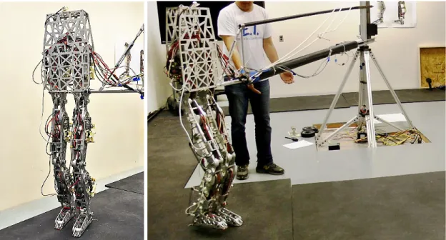
indi-cate the robot joints, and the yellow circular arrows indiindi-cate the actuators (motors) on the model. . . 6 1.4 The human-sized planar bipedal robot AMBER 3. It is 148 cm tall, weights
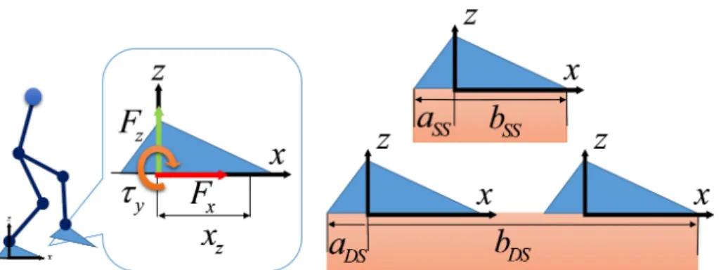
33.4 kg, with actuated hip, knee, ankle joints and passive toe, heel joints. It is capable of performing walking with multiple domains (e.g. walking with foot rolling motion). c2016 IEEE. Reprinted with permission from [1]. . . 11 2.1 The human-sized planar bipedal robot: AMBER 3. . . 18 2.2 The ZMP positionxz, ground reaction forces, and the corresponding ZMP
boundaries a and b in single support (SS) and double support (DS) are shown. Reprinted with permission from [1]. . . 20 2.3 A comparison of ZMP trajectories (left) and joint tracking profiles (right)
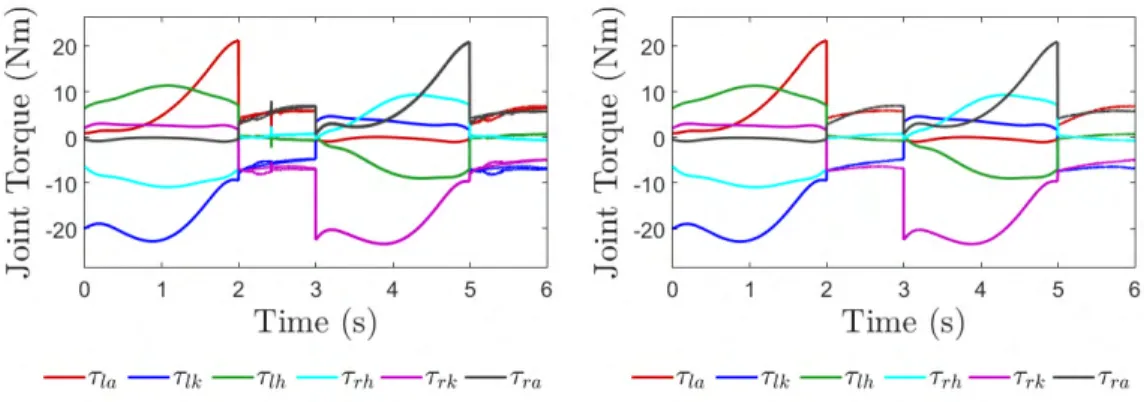
from two different simulations of the proposed method: in simulation (1) the unified QP with terminal constraints on the COM is used and in simu-lation (2) the terminal constraints are not used. Reprinted with permission from [1]. . . 32 2.4 Joint torques from the simulation of the proposed unified QP with (left)
and without (right) terminal constraints on the COM. Reprinted with per-mission from [1]. . . 33 2.5 Ground reaction forces of the simulation using the proposed unified QP
with (left) and without (right) COM terminal constraints. Reprinted with permission from [1]. . . 33 2.6 The walking tiles of a half gait cycle from a trajectory tracking
experi-ment in which AMBER 3 took 383 steps without falling using trajectories produced by the proposed method. Reprinted with permission from [1]. . . 34
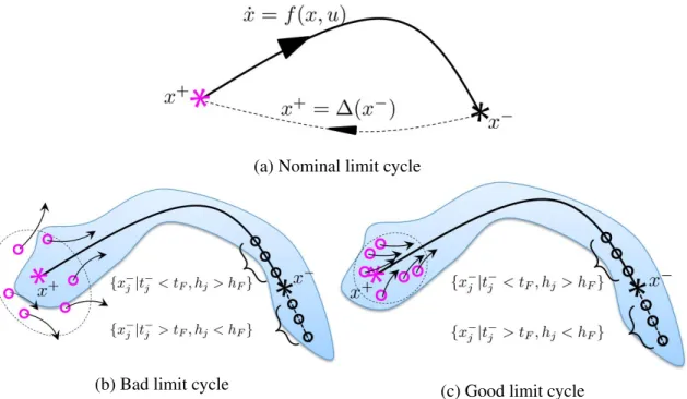
2.7 The joint tracking results from a trajectory tracking experiment in which AMBER 3 took 383 steps without falling using trajectories produced by the proposed method. Reprinted with permission from [1]. . . 34 3.1 The schematic of a nominal limit cycle, and the examples of ‘Bad’ and
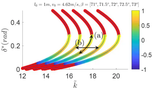
‘Good’ limit cycles in terms of how far the post-impact states (due to step height uncertainties) deviated from the nominal limit cycle. The shaded region indicates the region of attraction of the trajectory. . . 40 3.2 The schematic of a SLIP running model. TD indicates the touch-down
event and LO indicates the lift-off event. . . 43 3.3 The fixed points for different touch-down angles (β) and the same v0 =
4.62m/s. Each point indicates that there is a limit cycle of the SLIP run-ning model. Its color indicates the ev of its Poincaré map (Red indicates
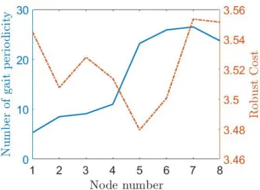
the fixed point is unstable). . . 45 3.4 The gait periodicity under step height uncertainties versus the robust cost
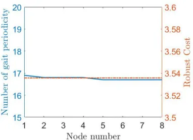
using step-time sampling (Eq. (3.2)) of fixed points listed in Table 3.1. . . 46 3.5 The gait periodicity under step height uncertainties versus the robust cost
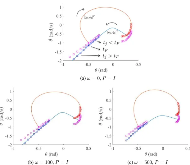
using step-time sampling (Eq. (3.2)) of fixed points listed in Table 3.2. . . 47 3.7 The schematic of a compass gait robot. . . 49 3.6 The phase portraits solved using Eq. (3.3) with the same set of stepping
time sampling (in the range oftF ±10%tF), the modified distance
mea-sure (Eqs. (3.6) and (3.7)), and different weighting ω for the robust cost function. The lines/curves spanned by post-impact states (pink markers) and pre-impact states of both legs (blue and red markers) become shorter towards to the nominal trajectory whenωis increased. . . 50 3.8 Walking 1000 steps on the terrain with uniform randomized slope angle
∈ [4.23o,9.23o] (Nominal slope angle: 5o). It shows that the pre-impact
states and post-impact states on the phase portraits (the end of red and blue trajectories) match the contour (the black lines connect the markers) predicted by the solution from the proposed robust trajectory optimization. 53
4.1 The human-sized planar bipedal robot AMBER 3 (left). It is 148 cm tall, weights 33.4 kg, with 6 active degree of freedoms at hip, knee and ankle joints, capable of performing walking with multiple contact domains (e.g. walking with foot rolling motion). It has passive toes (right) with the tor-sional springs (circled by the bright blue loop). Reprinted with permission from [2]. . . 56 4.2 The schematic of a bipedal robot with a floating base. Reprinted with
permission from [2]. . . 57 4.3 The walking tile of the generated gait with SACC. Reprinted with
permis-sion from [2]. . . 69 4.4 The walking tile of the generated with NSCC. Reprinted with permission
from [2]. . . 69 4.5 The walking tile of the generated gait with OSS. Reprinted with permission
from [2]. . . 70 4.6 The angular trajectory comparison between human data, gait SACC and
gait SACC with the kinematic optimization. Reprinted with permission from [2]. . . 71 4.7 The walking tiles of the experiment using the bipedal robot AMBER 3 [3]. 71 5.1 The schematic (a directed graph) of the contact sequence from human data. 78 5.2 The schematics of slope walking and stair walking. . . 84 5.3 An example of a smooth curve combined by two cubic splines as the profile
of the desired height of the foot clearance constraint. . . 87 5.4 An example to use the desired height profile for the constraint of swing
ankle (the top vertex of the triangle) height to increase the foot clearance. . . 88 5.5 The sparsity pattern of the Jacobian matrix of the constraints. The makers
indicate the nonzero elements.. . . 90 5.6 The walking tiles of the generated level-walking using HZD gait
optimiza-tion. . . 92 5.7 The walking tiles of up-slope walking. . . 92 5.8 The walking tiles of down-slope walking. . . 93
5.9 The walking tiles of stair walking. . . 94
5.10 The angular trajectory comparison between the optimization result of level walking and the human data. . . 95
5.11 The hip joint trajectory comparison for walking on slopes. In the leg-end−11.46o∗indicates the down-slope walking with smaller torso angle range:θtorso ∈[−0.15rad,0.15rad]. . . 97
5.12 The knee joint trajectory comparison for walking on slopes. . . 97
5.13 The ankle joint trajectory comparison for walking on slopes. . . 98
5.14 The histograms of level walking and down-slope walking results. . . 99
5.15 The histograms of up-slope and stair walking results. . . 100
6.1 The famous cart-table model to describe the LIPM for static balance (left), dynamic balance (center), and the schematic of the linear inverted pendu-lum model (right). . . 105
6.2 The analyzed tasks listed in the order of task complexity and the corre-sponding LIPM models for the CP-based step estimation. . . 111
6.3 The schematics of stationary tasks: Single-step recovery from the forward lean (left) and single-step recovery from the combination of forward lean and pull force (right). . . 112
6.4 Step location comparison between ICP and results in [4, 5] for Task (1).. . . . 115
6.5 Step location comparison between ICP and results in [6, 5] for Task (2).. . . . 115
6.6 Estimation error of step location (normalized by step length) for different walkers and difference tasks. . . 117
6.7 Normalized trajectories of COM, COM velocity, ICP, and EICP of the compass gait robot (CG) with respect to the normalized time , before the step is made (i.e. at¯t= 1.) . . . 118
6.8 Normalized trajectories of COM, COM velocity, ICP, and EICP of the kneed-gait robot with actuated ankles (KGFA) with respect to the normal-ized time , before the step is made (i.e. att¯= 1.) . . . 119
6.9 Normalized trajectories of COM, COM velocity, ICP, and EICP of human walking, before the step is made (i.e. at¯t = 1.) The shaded areas indicate the regions within a standard deviation. . . 120 6.10 The snapshot of human walking with severe slip occurred at the leading leg
(red) where the recovery step of the trailing leg (blue) was made behind the leading leg. . . 121
LIST OF TABLES
TABLE Page
1.1 The summary of the scopes and capabilities of the algorithms developed in different parts in this dissertation. . . 12 1.2 The capabilities of the algorithms of trajectory optimization developed in
this dissertation. All the methods we developed use the Hermite-Simpson Method (HSM) as the transcription method.. . . 15 2.1 Important simulation parameters. Reprinted with permission from [1]. . . 32 3.1 Stable fixed points of the SLIP running model along range (a) in Fig. 3.3
(β = 72o,v0 = 4.62m/s,l0 = 1m). . . 45
3.2 Stable fixed points of the SLIP model along range (b) in Fig. 3.3 (δ∗ = 0.2rad,v0 = 4.62m/s,l0 = 1m). . . 46
3.3 Important simulation parameters. . . 52 4.1 The list of the modified costs, stride lengths and double support
percent-age values for the initial guess, and generated gaits with different contact constraints. Reprinted with permission from [2].. . . 68 5.1 Comparisons between HZD and Contact-implicit trajectory optimization. . . 74 5.2 Important bounds for free variables . . . 87 5.3 Details of the HZD gait optimization for bipedal robot AMBER 3. . . 89 5.4 The summary of optimization results on different terrains . . . 91 6.1 Comparisons of the balance mechanism between the balance margin and
capture point for human balance strategies.. . . 110 6.2 Parameters of the walkers (values in parentheses indicate the standard
de-viation). . . 116 6.3 Estimation error of step location (normalized by step length) for
differ-ent robotic walkers. The values in the pardiffer-entheses indicate the standard deviation. . . 117
6.4 Estimation error of step location (normalized by step length) for human walking, walking with mild slip, and walking with severe slip. The values in the parentheses indicate the standard deviation. . . 118
1. INTRODUCTION
Robots have become more and more common in our daily life. It is not surprised to see robots can vacuum and mop our floors, the drones can follow us and take aerial videos and photos from the location or perspective that we cannot easily reach. For the automobiles, the driving-automation reaches to the level that seems so futuristic that the automated systems can take control of accelerating, braking, and steering so that the driver can let off the steering wheel on high way – at least for a short while.
Except wheeled and flying robots, legged robot is another form of robotic locomo-tion that has greater adaptiveness to human-living environment. Compared to the wheeled robots, legged robot can traverse along unstructured terrain without the need of the con-tinuous pathway, therefore can move or interact in the human environment (such as stair walking or ladder climbing). Legged robots in general also have larger payload than the flying robots. Among legged robots, bipedal robots and humanoids are suitable to perform human-robot collaboration and human services, as they possess the same locomotion type of humans’. However, those advantages come with their cost: as a highly articulated sys-tem, a bipedal robot’s floating base limits the force and torque it can exert to maintain the balance, the energetically efficient gait can be the mixture of different actuation conditions, and fast reactions are required when robot’s balance cannot be recovered via the original motion reference. Those challenges – although have been actively studying and exploring – make bipedal robots’ performance still not close enough to their biological counterparts. As part of our daily life, we use our vision to identify the path in front of us, and use it to guide our walking direction so that we will not stray out of the road. With years of learning and practice, we developed our walking gait such that we utilize heel-off (trailing leg) and knee-stretching to extend our step length, and handling the impact force with the
foot moving downward after heel-strike. When we accidentally lose our balance, even without too many practices, we will try our best to make a step after a step till we do not feel the risk of fall any more.
This dissertation focuses on developing model-based methods in bipedal robotics to get more understanding about those features which can be observed in human gait: 1) predictive behavior, 2) gait optimization, and 3) the stepping strategy. By exploiting dy-namics, planning and control, studying bipedal robots is also beneficial to the development of lower-limb wearable and rehabilitation devices for humans, which can potentially re-place the wheel chair and walker, or help users to restore their mobility.
In the following sections, first the big picture of bipedal robot automation will be pre-sented, and then the approaches which nicely capture those three features in the filed of the bipedal robotics will be introduced. The research objectives, the main topics of the dis-sertation, and the dissertation overview as well as the contributions will also be presented. 1.1 Bipedal Robot Automation as a Hierarchical Control System
For a bipedal robot to navigate in an environment autonomously, its control system can be illustrated as shown in Fig. 1.1. As the entire task is too complex to be handled within a single framework, the navigation task is usually broken down into three main components: 1) High-level motion planning, 2) Low-level tracking control, and 3) Model predictive control (MPC) to bridge the other two.
High-level motion planning. When an environment is given or is being perceived, the high-level motion planning is deployed to determine the sequence of the foot placement. This can be derived by the searching the environment as a grid-map using path-searching algorithms like A* with the collection of possible foot placements [7, 8], or the gait library solved by trajectory optimization [9, 10]. Usually this component take the longest com-putation time as the configuration space for a bipedal robot moving in an environment can
Figure 1.1: Controller overview as a hierarchical control system.
be really complex, and the task potentially can be achieved in numerous ways. As a result, either the simplest model is adopted, or this component is running in an off-line manner. Low-level tracking control. When the desired trajectory is planned, the low-level con-troller tracks the desired trajectory to achieve the walking motion. This needs to be achieved by continuously sensing the system’s states and making the corresponding cor-rection via control inputs. To control the robot to follow a trajectory precisely, it requires reliable software and hardware, and the precise model description (therefore Rigid Body Dynamics (RBD) is commonly used with the nonlinear controller design [11]). The sam-pling time is also crucial for the tracking performance (in general ranged in milliseconds). Model predictive control. As the bipedal system is with the floating base, even with the good low-level controller and nice hardware, the tracking result can still deviate from the original plan, since the contact condition can be easily perturbed by stepping impact or slippage due to small obstacles on the terrain, or even vibrations from the joint con-trol. This deviation can be accumulated step by step and cause the system reaches the
performance. In this case, model predictive control with moderate re-planning speed can be a powerful tool to correct the system’s behavior as the control input is derived from the best control sequence over a finite horizon, rather than just considering the state at the current time step. To solve the optimization with predicted states over the horizon on the flight, MPC is usually used with the model simpler than RBD.
With those building blocks, next we introduce several approaches of bipedal robot walking control studied in this dissertation, include the robot models, and how those ap-proaches achieve bipedal walking.
1.2 Approaches of Bipedal Robot Walking Control
To utilize the hierarchical control system introduced in the previous section, a method of walking control basically determines how the walking motion is generated, based on the selected model. With different perspectives to reason walking balance and stability, each walking control method has its own benefits and limitations, which will be briefly introduced in this section.
1.2.1 Bipedal Robot Models
There are various bipedal robot models that can be used to describe the dynamics of a bipedal robot system. The main differences between these models are the dimensions of the state, the type of control inputs, and the required assumptions (usually for simplifica-tion) so that a model can represent a bipedal walking system.
Linear Inverted Pendulum Model (LIPM).Linear inverted pendulum model (Fig. 1.2) is one of the classical simplified model that has been well-studied in bipedal robotics because of its simplicity, and its effectiveness to generate 3D walking motion. LIPM in general has the following assumptions:
• The dynamics only considers the motion of center of mass (COM) and the effect from the ground reaction force (GRF).
• The COM height is constant. This is also the key assumption as it decouples the dynamics of the COM horizontal motion from the COM vertical motion.
• In general it is assumed the LIPM has a perfect surface contact to the ground, thus there is no rotation in the COM motion. This is also an important assumption for the walking control using zero-moment point (which will be introduced in Chapter 2).
Figure 1.2: Schematic of the linear inverted pendulum model.
Though those assumptions help to greatly simplify the model and make it a lot easier to generate stable walking motion, it also make the system can only perform locomotion in a really restricted way. In addition, the generated walking using the LIPM may looks more unnatural, because the locomotion of humans and animals in general does not require those assumptions to be always hold.
Rigid Body Dynamics (RBD).Different from the LIPM, the rigid body dynamics aims to fully described the mechanical system with the very basic component – rigid body. RBD assumes each link of the robot model as a rigid body and is connected to other links with joints. In this way, a more complicated yet more accurate model can be derived to depict the system dynamics (as shown in Fig. 1.3).
Full-actuation vs. under-actuation. On one hand, when a system’s degrees of freedom are equal to its actuated joint number, the system is called full-actuated as the entire con-figuration of the robot can be fully controlled. LIPM in Fig. 1.2 is an example of the
Figure 1.3: Schematic of the rigid body dynamics. The black circular arrows indicate the robot joints, and the yellow circular arrows indicate the actuators (motors) on the model.
full-actuated systems. On the other hand, when a system’s degrees of freedom are more than its actuated joint number, the system is under-actuated. Take Fig. 1.3 for example, the system can not control the angle between the ground and the foot pad of the trailing leg since there is no actuator at the toe, therefore it can only affect that angle indirectly through the motors on other joints. Unlike LIPM, RBD can be used to describe different contact conditions including point and surface contacts, therefore is suitable to describe both full-actuated and under-actuated systems.
Feasible ground reaction force. For both surface and point contact, the resultant ground reaction force can be expressed with a normal force fn and a tangential force ft on an
exertion point (e.g. in Fig. 1.2fn=fy, andft=fx). There are two important conditions
to make a ground reaction force physically valid:
• The normal force should be always positive (i.e. pointing out of the contact surface.) • Based on the Coulomb friction model, for a non-sliding contact, the ground reac-tion force should be inside the fricreac-tion cone: |ft| ≤ µfn, where µ is the friction
1.2.2 Bipedal Robot Walking Control Methods
In this subsection we briefly introduce the state-of-the-art methods for walking control which are studied in this dissertation: zero-moment point, capture point, and hybrid zero dynamics.
Zero-Moment Point (ZMP). ZMP [12] is an important milestone in the development of bipedal robotics. The zero-moment point is the location where the ground reaction force can be expressed with zero-torque. By leveraging the concept of resultant force, it provides the dynamic balance criterionfor the full-actuated legged system (e.g. system with flat-foot contact): When the ZMP is inside the support polygon (the convex hull of the foot contact area), the system will not tip over. With the LIPM, the momentum equation can be expressed as a linear equation of COM and ZMP. With the ZMP reference determined from the sequence of foot placement, the walking control problem becomes the COM planning problem, where using model predictive control (MPC) with the LIPM to plan the COM walking pattern is a classical method which has been widely used for decades [13, 14, 15]. However, applying MPC and low-level control in sequence has its own pitfall: the limitations of the over-simplified LIPM also limit the system’s walking capability, therefore a lot of studies is also trying to generalize ZMP-based methods, such as methods using centroidal dynamics [16], or study using nonlinear simplified model [17]. Nevertheless, the dynamic balance criterion is still useful to ensure the walking balance while the system has surface contact to the ground.
Capture Point (CP).Extended from the ZMP-based method, capture point generalize it through the step-planning. Capture point [18] is the stepping location where the legged system can make a complete stop by stepping on it. Unlike the dynamic balance criterion that only quantifies the balance condition for the current stepping location, capture point can be generalized to N-step capture point forN = 0,1,2, . . . ,∞(the step location which
will need to take N steps to make the system into a complete stop.) Because the CP-based methods focus on fast stepping and COM (re)planning, so in general it can used for both full-actuated and under-actuated systems. Using capture point with the simplified model (like LIPM) enables the legged system to have fast reactions (replanning) against undesired disturbances, therefore it is well-known to handle push-recovery and walking on uneven terrains[19, 20, 21]. To overcome the limitation from the oversimplified model, there are more and more studies focus on generalizing CP-based method with the nonlinear simplified model [17].
Hybrid Zero Dynamics (HZD).Compared to ZMP-based and CP-based methods, HZD-based methods are on the other side of the spectrum [22, 23, 24]. Having the direct root in the locomotion generation of the passive robots (e.g. compass gait), hybrid zero dynamics aims to solve a dynamically feasible walking trajectory which can be executed periodically for the system under the stepping impact – a typical example of a hybrid system (which contains the continuous dynamics and discrete event). Because both passive and under-actuated systems require to solve the walking trajectory which can fully/partially run with its natural dynamics (i.e. the unactuated dynamics), one common approach to solve the walking trajectory for passive or under-actuated robots is using trajectory optimization. Trajectory optimization is a mathematical method to formulate a nonlinear program to solve the walking trajectory which optimizes a target objective function while satisfying a set of constraints such as the dynamical feasibility and the gait periodicity under the stepping impact (the later is also termed hybrid invariant condition). By leveraging the natural dynamics and imposing energy consumption or control effort into an objective function, the generated gaits can be energetically efficient and usually look more natural. However, since this method heavily relies on the accuracy of the dynamic model, and lacks balancing mechanism for non-surface contact, it is more challenging for HZD-based methods to achieve 3D walking motion.
1.3 Research Objectives – The Big Picture
As we mentioned, the purpose of this dissertation is to get more understanding about three important features of human gait: predictive walking behavior, gait optimization, and stepping strategy. In this section, we will explain the big picture, including how these fea-tures connect to i) control hierarchy, ii) related walking control methods, and iii) research objectives (denoted as R#, e.g., R1, R2) to be investigated in this dissertation.
1.3.1 Predictive Walking Behavior
Both bipedal robotics [25, 13] and biomechanics studies [26, 27] have shown the sig-nificance of predictive behavior for walking (e.g. watching over few steps ahead during walking to make sure the walking motion can be executed properly). In the examples of bipedal robotics [25, 13], the predictive behavior can be reasoned as a process using MPC with low-level control in sequence – a classical example of ZMP-based walking control. Traditionally, with given foot placements, the ZMP-based walker first runs MPC with the LIPM to plan the COM trajectory, and then the planned COM trajectory along with the trajectories of the other end effectors are tracked using the low-level controller. However, there is one major pitfall for using those controller in sequence: the models used in MPC (the simplified model) and the low-level controller (which is in general the RBD) are not the same, which lead to inconsistency issue. Therefore the research objective is:
R1. Improving the model consistency between model-predictive control and low-level control to enhance the predictive walking control.
1.3.2 Gait Optimization
Since optimizing a bipedal walking gait requires to exploit a bipedal robot’s dynam-ics as accurate as possible, the gait optimization using trajectory optimization – as one example of high-level motion planner – is usually performed in the offline manner. As
we briefly mentioned, with an objective function, a trajectory optimization formulates a the mathematical problem of walking trajectory generation as a nonlinear program to op-timize the objective function while satisfying a set of constraints of dynamical feasibility and periodicity of walking.
Among various methods of trajectory optimization in the literature, we mainly fo-cus on the methods usingdirect collocation framework [28, 29, 30, 31]. Direct colloca-tion method discretizes the trajectory of the system states and control inputs into discrete (collocation) points as independent decision variables, and solves the open-loop optimal control problem. The states and control inputs are related by the imposed constraints of the dynamic equations and the collocation constraints (which transcribe the states at the nearby collocation points as parameterized curves). Since most of the decision variables are only related to the adjacent ones, the direct collocation method makes the entire op-timization can be solved with sparse Jacobian matrices (of its constraints and objective function). Therefore this method can efficiently generate complex walking behaviors for complex robot systems (e.g. HZD-based walkers).
Form the control perspective, human walking is complex because the walking gait contains both the full-actuated and under-actuated walking phases (domains), which is an example of walking with multiple-domain. Our ultimate goal is to develop trajectory optimization algorithms to generate robust, energetically efficient and adjustable walking gaits so that the proposed algorithms can be used for lower-limb wearable robots, including prosthesis and exoskeleton. For this purpose, we plan to generate energetically efficient walking trajectories for a bipedal robot AMBER 3 (Fig. 1.4) with the following research objectives:
R2. Improve the robustness of walking gait for uneven terrains.
R3. Improve the state-of-the-art of trajectory optimization algorithms to generate energet-ically efficient walking gait with multi-domain.
Figure 1.4: The human-sized planar bipedal robot AMBER 3. It is 148 cm tall, weights 33.4 kg, with actuated hip, knee, ankle joints and passive toe, heel joints. It is capable of performing walking with multiple domains (e.g. walking with foot rolling motion). c 2016 IEEE. Reprinted with permission from [1].
R4. Impose additional constraints and cost so that the gait can be adjustable (for cus-tomization) and more human-like.
R5. Generate gaits for various terrains, including flat ground, slopes and stairs. 1.3.3 Stepping Strategy
The scope of the study for stepping strategy is slightly different from the other two. In the control hierarchy, the stepping strategy can be treated as an emergent mode which will only be triggered when the desired trajectory generated from the high-level planner and MPC can no longer maintain the balance. Additionally, stepping strategy can also be used as a regular walking control method which works with MPC and the low-level controller. As Capture Point (CP)-based methods have already shown the capability in different stud-ies [19, 20, 21], we focus on evaluating whether this method can be a potential tool for biomechanics and human rehabilitation. The research objectives are:
R6. Evaluate CP-based step estimation for human step-recovery from standing.
to exploit its performance.
R8. Evaluate CP-based step estimation for human walking with slip in different slip sever-ities.
1.4 Dissertation Overview
1.4.1 Main Parts of the Dissertation
In this dissertation, to present how we achieved those research objectives, we split those studies into three main parts: i) Quadratic program-based walking controller de-sign, ii) Trajectory optimization, and iii) Capture point-based method for human motion analysis. The scopes and the capabilities of the algorithms developed in those parts are summarized in Table 1.1.
Table 1.1: The summary of the scopes and capabilities of the algorithms developed in different parts in this dissertation.
Parts QP-based Trajectory Capture point
controller optimization -based analysis
Model RBD+LIPM RBD LIPM
Torque saturation 3 3 7
Balance criteria 3 7 3
Feedback control 3 7 7
Constrained optimal control 3 3 7
Foot-rolling motion 7 3 7
Step length estimation 7 7 3
Human motion analysis 7 7 3
In the following subsections, we will introduce each of the three main parts in the dis-sertation, including the corresponding chapters, their relations to each research objective and our contributions.
1.4.2 Quadratic Program-based Walking Controller Design
The main purpose of this part is to achieve the research objective R1, which is de-scribed in Chapter 2. There are several potential issues about the model mismatch when applying MPC and the low-level control in sequence. First, for MPC with the LIPM (COM planning), although the dynamic balance (i.e. ZMP constraints) over the horizon can be imposed into the constrained MPC, the planned COM is based on simplified model there-fore may not reflect the full dynamics of the bipedal robot. Second, for the nonlinear low-level control, although one can adopt a constrained optimal control to track the de-sired trajectory and impose the ZMP for the current time step, there is no guarantee that the state won’t enter the region where the ZMP constraint in the next time step will be vi-olated. To address those issues, by leveraging the fact that both the constrained MPC and constrained nonlinear control can be expressed as quadratic programs (QPs), we propose a QP-based controller design to combine both QPs into a single framework, with a synthesis equality constraint to equal the COM accelerations derived from the LIPM and RBD. In this way, the unified QP will simultaneously generate the COM motion (which satisfies the ZMP constraint over the horizon, and is with the feedback from the nonlinear RBD) and the control input (which can track alone the generated COM under torque saturation, dynamic balance, and Lyapunov stability constraints for the current time step).
1.4.3 Trajectory Optimization
For achieving research objectives (R2 – R5), Chapters 3 to 5 are the studies to explore different trajectory optimization algorithms with direct collocation framework.
optimization under terrain uncertainties, which is described in Chapter 3. In this work, by utilizing the structure of direct collocation method, the last few collocation points are used to sample the walking trajectory under terrain uncertainties – in this case, instead of sampling the walking trajectory with different step height similar to the works in [32, 33] (which complicate the trajectory optimization problem), we sample the walking trajectory with different step-time and design a robust cost function to improve the gait robustness without complicating the collocation framework.
To generate energetically efficient gait with multiple domains towards human-like mo-tion, both Trajectory optimization through contact [30] and Hybrid Zero Dynamics (HZD) gait optimization [24] are the main methods we use to develop our works further. In Chap-ter 4, we modify the optimization through contact to generate human-like level walking for objectives R3 – R4. With more accurate transcription (using Hermite-Simpson method), we compared the generated level walking with different contact constraints, and we also compared the optimization results to the human data. In Chapter 5, to reduce the sensi-tivity of the optimization to the randomized initial guess, the HZD gait optimization is implemented, which covers the objectives R3 – R5. With the modified contact constraints, the optimization can be generally used on different terrains include flat ground, different slopes and stairs. To analyze the sensitivity of the HZD gait optimization to the initial guess, the optimization performance with the randomized initial guesses under different terrain profiles are also evaluated and compared. The details of the trajectory optimization algorithms developed in this dissertation are summarized in Table 1.2.
1.4.4 Capture Point-Based Method for Human Motion Analysis
The works of this part is described in Chapter 6. The CP-based step estimation for step-recovery (objective R6) was studied by comparing the estimated step location to the human experimental results from the literature [4, 6] and the estimation from the optimization
Table 1.2: The capabilities of the algorithms of trajectory optimization developed in this dissertation. All the methods we developed use the Hermite-Simpson Method (HSM) as the transcription method.
Topics Robust trajectory Trajectory optimization HZD gait optimization through contact optimization
Model RBD RBD RBD Transcription method HSM HSM HSM Robustness under 3 7 7 terrain uncertainties Multiple (contact) 7 3 3 domains Contact sequence 7 3 7 generation
Sensitivity to initial guess medium high low
Level walking 7 3 3
Slope walking 3 7 3
Stair walking 7 7 3
using the simulation on a simplified model with MPC [5]. For the case of objectives R7 and R8, we compared the CP-based step estimation to the simulation data of robot walkers and the experimental data of human subjects. The results indicate that capture point can provide good estimations for human walking and walking with mild-slip (which is defined as the peak heel velocity (PHV) is<1.44m/s[34]).
1.5 Contributions
In this section, we summarize the contributions (denoted as C#, e.g., C1, C2) of all the studies introduced in the previous section.
Quadratic program-based walking controller design:
C1. Design a unified Quadratic Program (QP)-based controller design to integrate the elements from Model Predictive Control (MPC) for COM planning, and from rapidly
ex-based controller simultaneously solves for a COM trajectory that satisfies ZMP constraints over a future horizon while also producing joint torques consistent with instantaneous ac-celeration, torque, ZMP and RES-CLF constraints.
Trajectory optimization:
C2. Design a robust trajectory optimization using direct collocation with step-time sam-pling for terrain uncertainties. By utilizing the structure of direct collocation framework, the last few collocation points can be used to evaluate trajectory robustness and incorpo-rated into the proposed robust cost function to improve the gait robustness.
C3. Improve the trajectory optimization through contact for bipedal robot AMBER 3 with more accurate transcription: Hermite-Simpson method. Compare the generated level walking gaits with different contact constraints and human data.
C4. With modified contact constraints, extend the HZD gait optimization for bipedal robot AMBER 3 to generate walking gaits on various terrains including flat ground and differ-ent slopes and stairs. Compare the gait behavior to the human walking, and analyze the optimization sensitivity to the randomized initial guesses for different walking tasks.
Capture point-based method for human motion analysis:
C5. Validate CP-based step estimation for human behaviors. Results suggest that it can provide good step-estimation for human step-recovery from standing, walking, and walk-ing with mild slip (peak heel velocity<1.44m/s).
2. UNIFICATION OF LOCOMOTION PATTERN GENERATION AND CONTROL LYAPUNOV FUNCTION-BASED QUADRATIC PROGRAMS∗
2.1 Introduction
Numerical optimization plays an important role in the development of numerous walk-ing control approaches as the mathematics used to model bipedal robot control systems are often constrained, nonlinear, high-dimensional and incorporate impulse effects due to collisions between the robot and the ground. The usage of optimization in the control of robot walking can be categorized into “offline” optimizations which solve for walking gaits before the robot is turned on and “online” optimizations which are solved while the robot is walking. Examples of successful usage of offline nonlinear optimization include the efficient design of the Cornell Ranger [35], control output parameterization establish-ing (hybrid) system stability through Hybrid Zero Dynamics (HZD) and Human-inspired Control [23, 22], and direct state and input trajectory optimization [30].
On the other end of the spectrum, online numerical optimization – in the form of Quadratic Programs – has become increasingly popular in the control of walking robots due to the fact that some QP-based controllers with affine constraints can be solved in real-time [36] and that the structure of a Quadratic Program is well suited to handle a diverse set of problems in robotic walking. For example, in locomotion pattern generation appli-cations, Quadratic Programs can be used to solve Model Predictive Control problems to obtain center of mass (COM) trajectories consistent with Zero Moment Point constraints over a future horizon, as in [37, 13, 14, 15]. In this setting, the QP cost function is of-ten setup to minimize the error between future values of the COM and desired reference
∗This chapter is a slightly amended version of: c2016 IEEE. Reprinted, with permission, from
Ken-neth Y. Chao, Matthew J. Powell, Aaron D. Ames and Pilwon Hur, “Unification of Locomotion Pattern Generation and Control Lyapunov Function-Based Quadratic Programs”, American Control Conference,
Figure 2.1: The human-sized planar bipedal robot: AMBER 3.
values. On the other hand, in the context of nonlinear systems, QPs can be naturally cou-pled with control Lyapunov functions (CLFs) to form an optimal controller guaranteed to stabilize outputs corresponding to walking [38, 39]. In this setting, the quadratic cost func-tion minimizes actuafunc-tion effort and the constraints encode instantaneous ZMP and torque limits on the full nonlinear system.
Inspired by optimization-based approaches to locomotion, the proposed method com-bines two QPs: an adaptation of the MPC proposed in [14] for planning center of mass trajectories with the Linear Inverted Pendulum (LIP) model and an adaptation of [40, 41] for locally exponentially stabilizing a control Lyapunov function for the full nonlinear dynamics of the robot. The connection point is an equality constraint imposed on the dynamics of the center of mass which enforces that the instantaneous horizontal COM acceleration is the same in both the nonlinear system and the LIP model. With this bridge in place, the unified QP enjoys the advantages of both QPs: it resolves control actions which locally stabilize nonlinear control system outputs while ensuring that these control
actions are consistent with a forward horizon COM plan that satisfies ZMP constraints in the simplified model.
It is important to note that similar combinations of walking pattern generation methods and constrained, local nonlinear control have been proposed before. For example, in [42], the authors propose a similar QP which regulates the ZMP to zero over an infinite horizon using an optimal cost-to-go. In the present paper, however, the proposed controller solves a finite-time horizon MPC problem on the COM trajectory, which allows for both ZMP regulation and the enforcement of constraints on the evolution of the COM.
2.2 Controlling Robot Locomotion under ZMP Constraints
The Zero Moment Point (ZMP) is an important concept in the study of balance in robotic [12] and human locomotion [43]. For a legged robot with feet, the condition for dynamic balance (i.e. the robot not tipping over) is that the robot’s ZMP lies inside the robot’s support polygon. This section describes control methods for walking with ZMP constraints.
2.2.1 ZMP Constraints
As shown in Fig. 2.2, the ZMP positionxz in the sagittal plane can be expressed with
the ground reaction normal force Fz and moment τy , e.g. xz = −Fτyz in single support.
The ZMP constraints for dynamic balance can be described as:
a ≤ −τy/Fz ≤b (2.1)
where a ∈ {aSS, aDS} and b ∈ {bSS, bDS} encode the largest moment arms of the
support polygon in single support or in double support, as shown in Fig. 2.2. To satisfy instantaneous dynamic balance during walking, the inequality Eq. (2.1) on the ground reaction forces (GRFs) needs to be satisfied.
Figure 2.2: The ZMP position xz, ground reaction forces, and the corresponding ZMP
boundariesaandbin single support (SS) and double support (DS) are shown. Reprinted with permission from [1].
2.2.2 Nonlinear Robot Control System with ZMP Constraints
To achieve walking control with ZMP constraints and minimum control effort, a QP-based nonlinear controller with a Rapidly Exponentially Stabilizing Control Lyapunov Function (RES-CLF) [40] and force-based task [41] is adopted. This controller requires the full constrained dynamics described as the following form:
D(q)¨q+C(q,q˙) ˙q+G(q) = B JT h u F , ¯ B(q)¯u (2.2)
where q is the generalized coordinate,D(q)is inertia matrix, C(q,q˙)is Coriolis matrix, G(q)is gravity vector,Jhis Jacobian matrix of the contact constrainth(q),B is the torque
distribution matrix,F is the GRF vector (F = [Fx, Fz, τy]T in the sagittal plane) anduis
a set of actuator torques. Based on the extended inputu¯which includes joint torques and GRFs, instantaneous dynamic balance can be satisfied by solving the following quadratic
program: ¯ u∗ = argmin u ¯ uTHCLFu¯+fCLFT u¯ (CLF-QP) s.t. V˙ε(x)≤ −εVε(x) −bFz ≤τy ≤ −aFz (2.3) wherex= [q,q˙]T,H
CLF andfCLF are the quadratic and linear objective function
respec-tively. The first constraint establishes the exponential stability of output tracking where Vε(x)is a RES-CLF. The second inequality ensures that the instantaneous ZMP lies within
the support polygon.
However, the second inequality Eq. (2.3) is not guaranteed to be solvable, i.e. the robot can enter states for which there is no feasible solution to the ZMP constraints Eq. (2.3). This limitation is one of the primary motivators for combining local QPs with COM tra-jectory planning methods. In the following section, we show how to pose a Quadratic Program which solves for COM trajectories that satisfies ZMP constraints in the linear inverted pendulum model.
2.2.3 Linear Inverted Pendulum Model for COM Trajectory Generation
To simplify the ZMP tracking problem, one common approach is to generate a COM trajectory with the linear inverted pendulum model which tracks a desired ZMP trajectory. Model Predictive Control (MPC) is one method which has been employed in the literature for pattern generation with the Linear Inverted Pendulum Model (LIP model) [14, 15, 44]. The LIP model assumes a constant center of mass height. The resulting equation of motion forms a simple expression relating the ZMP and the horizontal COM,xc,
¨ xc=
g z0
wherez0is the constant COM height andgis the gravitational acceleration. To implement
MPC with the LIP model in Eq. (2.4), the discretized state space form of LIP can be derived as shown: xt+1 = 1 ∆T 0 ω2∆T 1 −ω2∆T 0 0 1 xt+ 0 0 ∆T ut (2.5) wherext = xct x˙ct xzt T
, ut = ˙zt, and∆T is the sampling time. With a given initial
state xt0 and a sequence of control inputs U¯ , the predicted sequence of statesX¯ for the nextN time-steps can be expressed asX¯ = ¯AX¯t0 + ¯B U¯ andA¯andB¯ can be derived recursively from Eq. (2.5). The predicted states then can be used to formulate an MPC-based quadratic program for COM trajectory generation:
¯ U∗ = argmin ¯ U ¯ UTHpU¯ +fpTU¯ (MPC-QP) s.t. Aiq,pU¯ ≤biq,p, (2.6)
where Aiq,p and biq,p include constraints on the evolution of the COM and ZMP over an
N time-step forward horizon. The advantage of COM generation with MPC is that it can be easily implemented in real-time. However, due to the simplification, there are some potential issues considering the implementation in full nonlinear dynamics, such as the fact that the control sequenceU¯ may not be feasible, or the generated COM trajectory for the simplified LIP model may not result in a feasible ZMP trajectory. These potential issues motivate a combined control method which takes advantage of the rapid pattern generation capabilities of the MPC-QP and ensures that the actual nonlinear control system satisfies instantaneous balance constraints.
2.3 Unification of Local Nonlinear Control and Walking Pattern Generation
In this section, we present the main formulation of the paper: a process for combining the nonlinear CLF-QP with the MPC-QP in a single control framework. Before the unifica-tion process is introduced, the setup of the CLF-QP and the MPC-QP, i.e. the construcunifica-tion of objective functions and constraints, will each be explained.
2.3.1 Control Lyapunov Functions
To realize ZMP-based locomotion, a local nonlinear controller in the form of the CLF-QP is used for tracking a set of control objectives [41]. For the controller construction, the rigid body equations of motion Eq. (2.2) can be expressed in the following general nonlinear control system form:
˙
x=f(x) +g(x)¯u, (2.7)
where x = [q,q˙]T. Input/output linearization [45] can be used to drive a set of control outputsy(q), ya(q)−yd(t)toward zero (whereya(q)are actual outputs,yd(t)are
time-based desired outputs). Here, the input/output relation for the (relative degree two) outputs y(q)is
¨
y =L2fy(x) +LfLgy(x)¯u+ ¨yd,Lf + ¯Au¯+ ¨yd, (2.8)
where “L” is the Lie derivative operator and A¯ denotes the decoupling matrix. Given a desired output dynamics y¨ = µ, a corresponding vector of joint torques and GRFs, u,¯ can be obtained through Eq. (2.8). In standard input/output linearization, this requires the inversion of A, however, as mentioned in [41], Eq. (2.8) can be resolved implicitly via¯ quadratic programming.
The goal in the design of µ is to drive y → 0. This motivates consideration of a linearized system with coordinatesη= [y,y˙]T which can be expressed as η˙ = F η+Gµ.
To exponentially stabilizeηto zero with a convergence rateε >0,µis designed to satisfy the following condition:
˙
Vε(η) =LfVε(η) +LgVε(η)µ≤ −εVε(η), (2.9)
where Vε(η) = ηTPεη is a RES-CLF, Pε is obtained by solving equation (47) in [38],
and LfVε(η) = ηT(FTPε +PεF)η, LgVε(η) = 2ηTPεG. A CLF-based Quadratic
Pro-gram (CLF-QP) of the form Eq. (2.3) is implemented to find the minimum control input µthat guarantees Lyapunov stability through the satisfaction of Eq. (2.9) and additional constraints.
2.3.2 CLF-QP Setup
This section describes the construction of the specific constraints and cost function considered for the local nonlinear CLF-QP of interest in this paper; for more details, see [41].
2.3.2.1 CLF-QP Constraints
The final form of the set of constraints to be used in the proposed CLF-QP variant is
Aiq,CLFu¯≤biq,CLF, (2.10)
Aeq,CLFu¯=beq,CLF, (2.11)
whereAiq,CLF andAeq,CLF are matrices andbiq,CLF andbeq,CLF are vectors of appropriate
dimension. The subscriptsiqandeqdenote inequality and equality, respectively.
(CLF-QP) optimization to ensure that the robot maintains dynamic balance. An additional constraint is included to ensure that the normal force applied to support foot is positive, i.e. Fz ≥ 0. Note that the ZMP constraints Eq. (2.1) and the normal force constraint
can be written as inequality constraints onu¯using the equations of motion Eq. (2.2), and thus be included in Eq. (2.10). Actuator saturation limits are likewise incorporated in Eq. (2.10) via the inequalities −umax ≤ u ≤ umax, whereumax is a vector of maximum
allowable torques. Finally, a CLF constraint is to used to drive the control objectives η →0. However, as aggressive control objectives and conservative torque limits can lead to infeasible systems of inequalities, the CLF constraint is relaxed [41] byδ > 0, resulting in
˙
Vε(η) = LfVε(η) +LgVε(η)µ≤ −εVε(η) +δ. (2.12)
The relaxation δ will be minimized in the cost function of the corresponding CLF-QP. The CLF constraint Eq. (2.12) together with the ZMP, normal force and torque constraints comprise the inequality constraints Eq. (2.10).
The equality constraints Eq. (2.11) enforce holonomic constraints h(q) = 0 corre-sponding to contact(s) between the robot and the ground through a constraint on the accel-eration
¨
h(q,q,˙ u¯) = 0. (2.13)
The vectorh(q)includes the horizontal and vertical components of one foot in the single support phase, and both feet in the double support phase.
2.3.2.2 CLF-QP Cost Function
The CLF-QP cost function is designed to balance the minimization of the controlµ and the relaxationδto the CLF constraint in Eq. (2.12)
argmin (¯u,δ)
pδ2+ ¯uTA¯TA¯u¯+ 2LTfA¯u¯ (2.14)
wherep > 0is a weighting factor. Note thatEq. (2.14) encodes the goal of minimizing µTµthrough Eq. (2.8). The CLF-QP cost function Eq. (2.14) and constraints Eq. (2.10)–
Eq. (2.11) are used in conjunction with elements of a walking pattern generation QP to form the unified QP described in Section 2.3.5.
2.3.3 Walking Control Objectives
This section describes the choice of control objectives, i.e.,ya(q)andyd(t), for
achiev-ing ZMP-based walkachiev-ing in the nonlinear system Eq. (2.2). To reduce the differences be-tween the LIP and the full nonlinear dynamic model, the height of the COM is regulated to a constant z0 > 0, and the desired torso angle with respect to inertial frame is set to
zero. In the single support phase, the desired orientation of the swing foot is set to zero (to ensure that the foot lands flat on the ground), and the desired horizontal and vertical com-ponents of the swing foot are smooth time-based polynomial functions with zero boundary velocities and accelerations. Finally, note that
¨
xc =L2fxc+LfLgxcu,¯ (2.15)
is the actual acceleration of the center of mass in the nonlinear system. To achieve forward walking, an equality constraint will be enforced onu¯to achieve a desired acceleration of the center of mass, i.e. L2fxc+LfLgxcu¯= ¨xdc. The value ofx¨dc will be determined through
the use of the LIP model for walking pattern generation, as described in the next section and Eq. (2.15) will subsequently be used as a bridge between the nonlinear robot dynamics and the LIP model.
2.3.4 LIP Model Predictive Control Setup
The CLF-QP – described by the constraints Eq. (2.10) and Eq. (2.11) and cost function Eq. (2.14) – provides a method of locally stabilizing control objectives in the full nonlin-ear robot dynamics while also ensuring the instantaneous ZMP constraints are satisfied. However, under the action of the CLF-QP alone, the robot can enter states for which there is no feasible solution to the ZMP constraints. This motivates the combination elements of the local nonlinear CLF-QP with elements of a Model Predictive Control QP for pro-ducing feasible ZMP trajectories over a forward horizon. The following sections describe the construction of the specific MPC-QP considered.
2.3.4.1 General MPC Setup
The MPC-QP solves a receding horizon problem using the discrete-time, LIP dynamics Eq. (2.5) with time-step∆T. The target walking behavior consists of alternative phases of single and double support. The target duration of the single and double support phases are TSS and TDS seconds, respectively. The number of discrete points in the plan is fixed to
beN = (TSS+TDS)/∆T. Similar toX¯ in Eq. (2.5), the predicted evolution of the ZMP,
xzt, COM,xct, and COM velocity,x˙ct, for the next N discrete points can be expressed as:
¯ Xz = ¯AzmpX¯t0 + ¯BzmpU¯ ¯ Xc = ¯AcomX¯t0 + ¯BcomU¯ ˙¯ Xc = ¯AcomVX¯t0 + ¯BcomVU¯ (2.16)
where A¯zmp, B¯zmp, A¯com, B¯com, A¯comV and B¯comV also can be derived recursively from
Eq. (2.5). As these expressions are affine in U¯, constraints on the evolution of ZMP and COM can be expressed as constraints onU¯.
2.3.4.2 MPC Horizon Computation
As mentioned previously, the COM trajectory planner will implement a receding hori-zon. The model predictive control problem will solve 2 phases into the future. In general, this means the problem will have 3 domains: one for the completion of the current phase (withN1 discrete points), one for the entire duration of the next phase (withN2 discrete
points) and one for the remainder (withN3discrete points), whereN1+N2+N3 =N. As
the target walking consists of alternating phases of single and double support, the values N1,N2andN3 will change depending on the current phase. Specifically, at a point in time
t during a single support phase, the number of discrete points in first domain isN1,SS =
(TSS −t)/∆T, the number of discrete points for next domain isN2,DS = (TDS)/∆T and
the third and final domain’s discrete point number isN3,SS =t/∆T. Similarly, at a point
in time t during a double support phase, the numbers of discrete points for the three do-mains areN1,DS = (TDS−t)/∆T,N2,SS = (TSS)/∆T andN3,DS =t/∆T respectively.
2.3.4.3 MPC Constraints
An equality constraint is imposed on the MPC-QP to enforce that the center of mass reaches the positionxgoal
c at the end of the trajectory with the terminal velocityx˙goalc .
Ad-ditionally, inequality constraints are imposed on the resultant ZMP trajectories to ensure that the ZMP lies within the support polygon throughout the duration of the plan.
Aeq,pU¯ =beq,p
Aiq,pU¯ ≤biq,p
where Aeq,p = [0N−1,1] ¯Bcom [0N−1,1] ¯BcomV beq,p = xgoal c −[0N−1,1] ¯AcomX¯t0 ˙ xgoal c −[0N−1,1] ¯AcomVX¯t0 Aiq,p = [ ¯Bzmp,−B¯zmp]T biq,p = [¯b−A¯zmpX¯t0,−a¯+ ¯AzmpX¯t0] T (2.18)
In Eq. (2.18),¯aand¯bboth include three ZMP boundary sequences, which are determined by the three domains in the horizon, with the corresponding support phase (single support or double support) and step length (N1,N2, orN3). For example, the frontal ZMP
bound-ary of the horizon¯awill be[¯aSS,¯aDS,a¯SS+ 0.5Lstep]T if it is in single support, anda¯will
be[¯aDS,a¯SS+ 0.5Lstep,¯aSS + 0.5Lstep]T if it is in double support, whereLstepis the step
length.
2.3.4.4 MPC Cost Function
The cost function balances the goals of minimizing control effort, achieving ZMP tra-jectory tracking, and driving the COM position to the desired location for next stepping. This formulation is similar to the one used in [15]. The sequence of control inputsU¯ then can be derived by solving the following optimization problem:
argmin ¯ U∗ ω1U¯TU¯ +ω2|X¯z−X¯zgoal| 2 (2.19) s.t. a¯≤X¯z ≤¯b (ZMP) xct0+N =x goal c (COM) ˙ xct N = ˙x goal c (COM Vel.)
whereω1andω2are weighting factors,X¯zgoal is the desired ZMP trajectory,xgoalc andx˙goalc
are the desired COM terminal location and velocity att=t0+N respectively,¯aand¯bare
ZMP boundary vectors of the horizon. Using the equation in Eq. (2.16), the cost function in Eq. (2.19) can be expressed as follows:
argmin ¯ U∗ 1 2 ¯ UTHpU¯+fpTU¯ (MPC-QP) s.t. Aeq,pU¯ =beq,p Aiq,pU¯ ≤biq,p (2.20) where Hp = 2ω1I+ 2ω2B¯TzmpB¯zmp fp = 2ω2[ ¯AzmpX¯t0 −X¯ goal z ] TB¯ zmp (2.21)
Note that the desired ZMP sequence X¯zgoal and the desired terminal COM position xgoalc are calculated based on a horizon which changes over time.
2.3.5 Main Result: Unified QP Combining Pattern Generation and ZMP-based Walking Control
Using the building blocks of the quadratic programs for pattern generation and ZMP-based locomotion with RES-CLF QP, the proposed controller synthesizes all elements into a unified quadratic program: