Measuring financial risk

(1)

Universidad Carlos III de Madrid

TESIS DOCTORAL

T´ıtulo de la tesis:

Measuring Financial Risk

Autor

:

Maria Rosa Nieto Delfin

Directora

: Esther Ruiz

Doctorado en Econom´ıa de la Empresa y M´

etodos Cuantitativos

Departamento de Estad´ıstica

Universidad Carlos III de Madrid

Getafe, Mayo de 2010

(2)

TESIS DOCTORAL

T´ITULO DE LA TESIS:

Measuring Financial Risk

Autor: Maria Rosa Nieto Delfin

Directora: Esther Ruiz

Firma del Tribunal Calificador:

Nombre y Apellidos Firma

Presidente ROSA ELVIRA LILLO RODRIGUEZ

Vocal HENRYK GZYL BUCHHOLZ

Vocal RICARDO CAO ABAD

Vocal ANGEL LEON VALLE

Secretario ANDREAS HEINEN

Calificaci´

on:

(3)

2

(4)

Acknowledgements

First of all, I would like to thank my supervisor Esther Ruiz for her patience, under-standing, help and teaching along these last years. Fortunately, I learned a lot from her, not only about the subject of this thesis, but also as a person. I really appreciate all the time she spent working with me, because without her support I would have not finished this work.

I’m very grateful to the professors of the Statistics Department for their support and help with all the issues related to the teaching practice, specially with the coordination assistantship.

I would also like to show my gratitude to the Spanish Ministry of Education and Science and to the education and culture section of the Community of Madrid for financial support. In particular, I would like to thank Esther Ruiz for allowing me to participate in the research projects SEJ2006-03919 and ECO2009-08100.

As I promised, I will specially mention two of the most important people I knew in Spain, my friends Santi and Alex. I really do not have words to thank them for all the support and advices they gave me and also for the time they dedicated to help me with uncountable problems. I always said, as a joke, that they were my ”co-advisors”. Thanks a lot, I know we will be friends forever.

I also want to thank the rest of my friends for being my family here. Ana, Alba, Pepa, Ester, Ana Laura, Peter, Adolfo, Andre, Hugo and Silviu. Thanks for the talks, the moments, the anecdotes and specially for the company. You can always rely on me. I dedicate my thesis to the three most important columns of my life, my grandmother Rosa Montero, my aunt Rosa A. Delfin and my father Isaac Arturo Nieto, because they though me all the fundamental lessons that I keep in my heart and that I try to apply everyday that I live. I will also want to thank my sisters Adriana, Teresa and Larissa and my brother Isaac Antonio for standing next to me along all these years. Thanks for taking care of me and for your advices. My very special mention is for the fundamental part of my life, my six kids. My nieces Angie, Tazi, Yoryis and Sarita and my nephews Nemo and Puny, you are the reason why my life is happier now. Since you were born, everyday is different and full of joy. I am so grateful of having you with me and I am happy that very soon I will be around for watching you grow.

(7)

Resumen

La importancia de la administración de riesgos viene de la necesidad que tienen los bancos y entidades financieras de tener una reserva de capital que les permita afrontar sus obligaciones financieras. El concepto de riesgo es muy amplio debido a que hay diferentes grupos de personas interesados en la bolsa de valores y cada grupo tiene su propia actitud con respecto al riesgo; ver Granger (2002). El riesgo financiero puede ser clasificado en riesgo de crédito, de liquidez, operacional, legal y de mercado. Riesgo de crédito es el riesgo que se adquiere cuando las contrapartes no son capaces de cumplir con sus obligaciones contractuales. Riesgo de liquidez es la inhabilidad para efectuar pagos contra´ıdos con anterioridad. El riesgo operacional está relacionado con acci-dentes técnicos y humanos, el riesgo legal surge cuando una transacción no puede ser legalmente completada. Finalmente, el riesgo de mercado es el riesgo asociado con cam-bios inesperados en los rendimientos en intervalos cortos de tiempo. En esta tesis nos centraremos en el riesgo de mercado; ver Jorion (1990) y Duffie and Pan (1997).

Existen dos problemas importantes cuando se trata de estimar el riesgo. Primero, se deben considerar medidas de riesgo con propiedades te´oricas adecuadas. Segundo, se deben escoger estimadores con propiedades estad´ısticas apropiadas.

Una de las medidas de riesgo más populares es el Valor en Riesgo (VaR). El VaR aparece como consecuencia de algunos resultados adversos a lo largo de la historia que forzaron a las agencias reguladoras de la actividad financiera a buscar una forma cuantitativa de definir el riesgo asociado a una posición en el mercado. El VaR se define como la m´ınima pérdida potencial que, en el 100α% de los peores casos con α∈(0,1), puede tener una cartera en un horizonte temporal determinado. Entre las principales ventajas del VaR están su simplicidad, aplicabilidad y universalidad; ver Jorion (1990,

(8)

Contents 7

1997) y Embrechts et al. (2000). Sin embargo, tiene importantes limitaciones desde el punto de vista te´orico. El inconveniente mas importante de esta medida, es que el VaR de una cartera diversificada puede ser mayor que la suma de los riesgos de las carteras individuales.

Como resultado de las limitaciones del VaR como medida de riesgo, Artzner et al. (1997) definieron lo que se conoce como Medidas de Riesgo Coherente. Artzner et al. (1999) propusieron el Tail Conditional Expectation o también llamado Conditional Value at Risk (CVaR). El CVaR mide la pérdida esperada en que se incurrirá en el 100α% de los peores casos. Adicionalmente, Acerbi and Tasche (2002) proponen el Expected Shortfall (ES) como medida de riesgo coherente. Es importante mencionar que el ES es igual al CVaR cuando la distribución de los rendimientos es continua.

Sin embargo, el VaR sigue siendo la medida mas utilizada por los bancos e insti-tuciones financieras. Además, una adecuada estimacin del VaR es fundamental para estimar el ES. Por lo tanto, existe un gran interés en su estimación. Hay varios temas relacionados con la estimación del VaR y del ES que serán considerados en esta tesis. Primero, la decisión acerca del estimador que se utilizará. Segundo, se necesita escoger el nivel α para el VaR y el ES as´ı como el periodo sobre el cual se calcularán ambas medidas. Finalmente, es también importante tener medidas sobre la incertidumbre asociada con la estimación.

En el Cap´ıtulo 2 se revisan varios estimadores para el VaR y el ES. Las ventajas y desventajas de dichos estimadores son ilustradas implementándolos a los rendimientos diarios del S&P500. También se revisan y comparan mtodos alternativos para pro-bar la precisión de las estimaciones del VaR y del ES. El objetivo en este Cap´ıtulo es describir las principales contribuciones en estimación de ambas medidas de riesgo actualizando estudios previos. Además, extendemos estos estudios con una comparacin de métodos mas exhaustiva. Se consideran varios modelos alternativos para la varianza condicional y para la distribución de los errores. Finalmente, también se comparan algunos estimadores propuestos en la literatura para estimar el ES.

(9)

Contents 8

requerido 1%, se consideran puntos diferentes de la cola de la distribución de los rendimientos, por ejemplo, el 5% y el 10%. Se implementan los procedimientos de esti-mación descritos en el Cap´ıtulo 2 y se comparan los resultados con los que se obten´ıan al 1%. Adicionalmente, se analizan los procedimientos utilizados para predecir el VaR y el ES en horizontes de predicción distintos a un periodo hacia adelante. El comité de Basilea requiere que el VaR sea reportado en periodo de 10 das. Por esta razón, el análisis se ha enfocado en predecir en este horizonte. Se han implementado y comparado distintos procedimientos a la serie de rendimientos diarios y quincenales del S&P500.

Finalmente, en el Cap´ıtulo 4 se toma en cuenta la incertidumbre asociada con la estimación del VaR y del ES mediante la construcción de intervalos de predicción. Se supone que los rendimientos están bien representados por modelos de tipo GARCH y se propone una extensin del procedimiento bootstrap de Christoffersen and GonÇ alves (2005) mediante la incorporación de un segundo paso bootstrap en la estimación del per-centil de la distribución condicional de los residuos estandarizados. Además, siguiendo la propuesta de Ho and Lee (2005), se consideran intervalos de predicción bootstrap que superan las limitaciones de los intervalos de predicción tradicionales. Se muestra que nuestro procedimiento bootstrap mejora el rendimiento de los intervalos de predicción para el VaR y el ES al tener coberturas más cercanas a las nominales.

(10)

Chapter 1 Introduction

1.1 Motivation

The importance for risk management in financial institutions comes from the necessity of having a reserve of capital for facing their financial obligations. The concept of financial risk is very wide since there are different groups of people interested in the money market and each group has its own attitude about risk; see Granger (2002). Financial risk can be classified into credit, liquidity, operational, legal and market risks. Credit risk is the risk faced when the counterparties are unable to fulfill their contractual obligations while liquidity risk refers to the inability to meet payments obligations, operational risk is related to human and technical accidents and legal risk arises when a transaction cannot be legally accomplished. Finally, market risk is the risk associated with unexpected changes in returns over short time horizons; see Jorion (1990) and Duffie and Pan (1997). In this thesis, we focus on market risk. In a simple situation, if we buy an asset at price Pt−1 at time t−1, and sold it at price Pt at time t, we get a

return calculated as the first difference of logarithm of prices,Rt= log(Pt)−log(Pt−1).

In t−1, Rt is unknown and the risk is caused by this uncertainty. The return at time t can be considered unsatisfactory by the investor when it is negative or inferior to the return of some kind of governmental bond.

There are two main issues involved in estimating risk. First, one should consider measures of risk with adequate properties from a theoretical point of view. Second, once we decide how to measure risk, we should choose estimators of the corresponding

(11)

1.1. Motivation 10

measure with appropriate statistical properties.

There are different measures of market risk proposed in the literature. Luce (1981) suggests to measure risk by assigning different weights to the two halves of the dis-tribution of returns. Therefore, if f(R) is the density of returns, the risk is given by Riskt=A1 ∞ Z 0 R_tθf(R)dRt+A2 0 Z −∞ |Rt| θ f(R)dRt (1.1)

where A1, A2 ≥ 0 and θ > 0. Depending on whether f(R) is the marginal density or

the density of Rt conditional on past observations, we obtain marginal or conditional

moments. In this thesis, we consider conditional distributions of returns because it is a more efficient use of the information contained on the data. When the weights in (1.1) are equal, we have the class of volatility measures given by

Vt(θ) = E t−1 h |Rt−µt| θi (1.2) where µt = E

t−1[Rt] and the t−1 under the expectation means that it is taken

condi-tional on the information available up to timet−1. Vt(θ) includes the two most popular

measures of risk, namely the variance, when θ = 2, and the mean absolute deviation, when θ = 1. However, only when the utility function is quadratic or the distribution of returns is Normal or log-Normal, the variance is an appropriate measure; see Tobin (1969), Tsiang (1972), Machina and Rothschild (1987) and Levy (1992). The assump-tion of Normal condiassump-tional distribuassump-tion could be adequate in some financial returns. However, the utility cannot be assumed to be quadratic as the investor has different at-titudes depending on whether the returns are over or under their means. In that sense, there is uncertainty in the upper part of the distribution, but the risk only exists in the lower part, which means that the investors do not diversify for reducing the possibility of an unexpected positive return, just if it is negative; see Granger (2002). Therefore, measures based onVt(θ) are not in general adequate to measure risk.

One of the most popular alternative measures of risk is what is known as the Value at Risk (V aR). The V aRappears as a consequence of some adverse results along history which force the agencies that regulate financial activity to look for a quantitative way to

(12)

1.1. Motivation 11

define the risk associated to a position in the market. TheV aRis defined as the minimal potential loss that a portfolio can suffer in the 100α% worst cases with α ∈ (0,1), on some fixed time horizon. In particular, the V aRis given by

V aRα_t = sup r | P t−1[Rt≤r]≤α . (1.3)

Among the main advantages of the V aRare simplicity, wide applicability and uni-versality; see Jorion (1990, 1997), and Embrechts et al. (2000). Consequently, since the 80’s, the regulatory agencies have used theV aRto measure the risk of financial institu-tions. According to the Basel Committee on Banking Supervision, banks are required when calculating V aR. They require to compute the V aRfor α= 0.01 and for returns corresponding to 10 trading days. Furthermore, the V aR should be computed with observations corresponding to at least one year. However, the V aR has fundamental limitations from the point of view of its theoretical properties. The most important of them is that theV aRof a diversified portfolio can be greater than the sum of theV aRs

of the individual portfolios; see Acerbi and Tasche (2002). Furthermore, theV aRdoes not measure losses exceeding itself. Consequently, we can have two distributions with heavy tails and the sameV aR, but the losses that exceed V aR could be totally differ-ent; see Basak and Shapiro (2001) and Yamai and Yoshiba (2005) for both theoretical and practical discussions on the tail risk of V aR. In order to exemplify this, Acerbi et al. (2001) used the next paradox: consider a portfolio A (made of long positions) of value 1000 euro with a maximum downside level of 100 euro and suppose that the worst 5% cases on a fixed time horizon T are all of maximum downside. V aR at 5% on this time horizon would then be 100 euro. Consider now another portfolio B again of 1000 euro which on the other hand invests also in strong futures positions that allow for a potential unbounded maximum loss. We could choose B in such a way that its V aRis still 100 euro on the time horizon T. However, in portfolio A the 5% worst case losses are all of 100 euro and in portfolio B the 5% worst case losses range from 100 euro to some arbitrarily high value. Additionally, from the point of view of optimization, the

V aR is not useful because it is not convex; see Szeg¨o (2002).

As a result of the limitations of theV aR as a measure of risk, Artzner et al. (1997) define what is known as Coherent Measures of Risk. A Coherent Measure of Risk,ρ(·),

(13)

1.1. Motivation 12

must satisfy the following properties:

(i) Monotonicity: ∀ R, S returns of two assets of portfolios, such that R ≤ S =⇒

ρ(R)≤ρ(S) ;

(ii) Positive Homogeneity: ∀c≥0 and ∀R, ρ(cR) =cρ(R) ;

(iii) Translation invariance: ∀r∈_R and ∀R, ρ(R+r) =ρ(R)−r;

(iv) Subadditivity: ∀ R, S, ρ(R+S)≤ρ(R) +ρ(S).

The monotonicity condition implies that if the return of a portfolio is smaller than that one of another portfolio, then the portfolio with larger return will have larger risk. The second property means that if the return is multiplied by a constant, the risk will change in the same proportion. The third property means that if you invest in a risk free asset, the faced risk will decrease in this amount. The most distinctive of these properties is the Sub-additivity which implies that a portfolio which is made of portfolios would have at most the same risk as the sum of the risks of sub-portfolios thanks to risk diversification. Note that, as we mentioned above, theV aRis not sub-additive.

Wang et al. (1997) propose measures of risk with distortion functions which, under certain conditions, are coherent; see Wang (1998) for one of this measures. Later, Artzner et al. (1999) propose the Tail Conditional Expectation or Conditional Value at Risk (CV aR). The CV aR,that measures the expected loss in the 100α% worst cases, is given by

CV aRα_t = E

t−1{Rt|Rt≤ −V aR

α

t)}. (1.4)

The CV aR is a coherent measure of risk when it is restricted to continuous

dis-tributions. However, it can violate sub-additivity with non-continuous disdis-tributions. Consequently, Acerbi and Tasche (2002) propose the Expected Shortfall (ES) which is given by

(14)

1.1. Motivation 13 where λ ≡ P t−1[Rt≤ −V aR α t]

α ≥ 1. Note that CV aR = ES when the distribution of

returns is continuous; see Giannopoulos and Tunaru (2005). However, the ES is still coherent when the distribution of returns is not continuous. Another advantage of the

ES when compared with the more popular V aR, is that it is free of tail risk in the sense that it takes into account information about the tail of the underlying distribution. The use of free tail risk measures avoids extreme loss in the tail. Therefore, the ES

is an excellent candidate for replacing V aR for financial risk management purposes. However, the effectiveness of ES depends on the stability of its estimation and the choice of efficient backtesting methods; see Fabozzi and Tunaru (2006).

Although the V aR has important theoretical limitations as a measure of risk, Danielsson et al. (2005) explore the potential for violations of the V aR subadditivity and conclude that for most practical applications the V aR is subadditive. Therefore, according to this analysis, there is no reason to choose a more complicate risk measure than the V aR solely for reasons of coherence. Furthermore, Danielsson et al. (2006) show that for heavy tailed distributions, as those observed in financial returns, the choice of downside risk measures does not seem to matter much as all of them (includ-ing V aR and ES) order heavy tailed risk in a similar manner. In any case, the V aR

is still the measure most extensively implemented by banks and financial institutions. Furthermore, an adequate estimation of the V aR is fundamental to estimate the ES. Therefore, there is a huge interest on its estimation. There are several issues of interest related with the estimation of the V aR and ES that will be considered in this thesis. First, one has to decide about the particular estimator to be implemented. Second, the level of theV aR and theES has to be chosen as well as the period for computing them. Finally, it is also important to have measures of the uncertainty associated with their estimation.

(15)

1.2. Value at Risk and Expected Shortfall 14

1.2 Value at Risk and Expected Shortfall

1.2.1 Alternative estimators

Once one decides about which measure of risk to implement, it is necessary to estimate it. Although the Basel Committee establishes that financial institutions must use the

V aR as a measure of risk, they are free to choose the estimation method. There are a very large number of estimation methods proposed in the literature to estimate theV aR

and a relative smaller number of proposals for theES; see Manganelli and Engle (2001), GenÇ ay and SelÇ uk (2004), Angelidis et al. (2005), Kuester et al. (2006), Lima and Néri (2007) and McAleer and da Veiga (2008) for surveys on V aR and ES estimation.

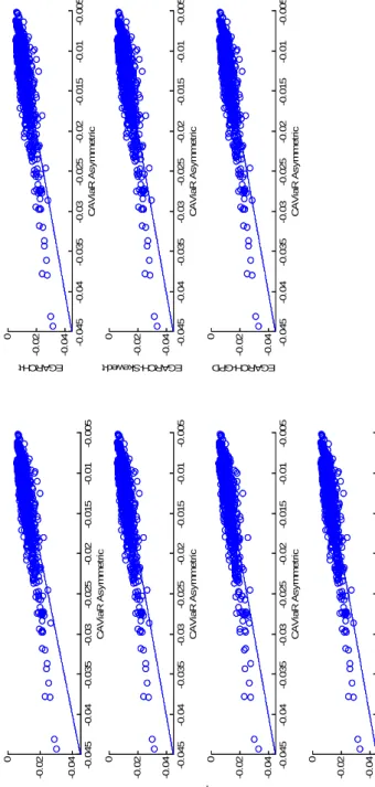
V aR estimators can be classified in nonparametric, semiparametric and paramet-ric. Some of the most popular nonparametric methods are Historical Simulation (HS) and Bootstrap procedures that do not make any distributional assumption on the dis-tribution of returns. On the other hand, there are many proposals in the literature of parametric specifications of the conditional mean and variance and the conditional error distribution implemented to estimate the VaR and ES, as for example, the Riskmet-rics, GARCH orCAV iaRspecification. Finally, some examples of the semiparametric methods are those based on Extreme Value Theory (EV T) and Feasible Historical Sim-ulation (F HS). Both methods assume GARCH models for the conditional volatility but differ in the way the quantile of the distribution of returns is calculated.

After the V aR and ES are estimated, one needs to measure their accuracy. The Basel Committee proposes a backtesting procedure which consists on the comparison between the nominal V aRlevel, α, and the proportion of actual returns which are less than or equal to theV aR forecasts. Many backtesting procedures have been proposed afterwards in the literature; see, for example, Kupiec (1995), Christoffersen (1998), Christoffersen and Diebold (2000), Christoffersen et al. (2001), Dowd (2001), Engle and Manganelli (2004) and Berkowitz et al. (2006) for theV aR and Berkowitz (2001) and Kerkhof and Melenberg (2002) for ES. These backtesting procedures are designed to discriminate whether a particular estimator is accurate. However, when several alternative accurate estimators are available, one also wants to choose which is the

(16)

best among them. There are several proposals to accomplish this task, as for example, Lopez (1999), Sarma et al. (2003), Giacomini and Komunjer (2005), Bao et al. (2006), Giacomini and White (2006) and Angelidis and Degiannakis (2007).

Very recently, Wong (2010) proposes the tail risk statistic for backtesting. This statistic provides information on the risk faced by investors beyond theV aRboundary. Note that the tail risk statistics is closely related with the V aR and ES but is an alternative measure of risk which we will not consider further in this thesis.

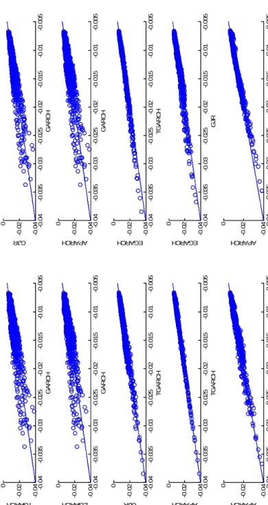
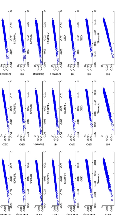
Our first goal is to make an updated and detailed revision of the literature on estimation and backtesting of V aR and ES. By implementing alternative procedures to the same series of returns, we will analyze whether there are significant differences between the estimates obtained by alternative procedures and, in this case, whether it is more important to have an appropriate specification of the conditional variance or the distribution of returns.

1.2.2 Alternative horizons and levels

In practice, when a risk manager faces the problem of measuring the risk of a portfolio by estimating theV aR or the ES, he must take into account that the final conclusion will change depending on the α level, the horizon and the sample period of the data. Therefore, these three factors must be fixed at the beginning of the analysis depending on the necessities of the financial institution.

Most of the literature related with the estimation of theV aRandESdeals with one-step ahead predictions. However, according to the amendments of the Basel Committee, the V aR should be reported for a 10 days horizon, in such a way that the portfolio manager has time to rebalance his portfolios in case it is needed. Furthermore, there are situations in which measurements of risk are required for longer horizons, for example, financial institutions with long term liabilities like pension funds and life insurance com-panies, corporations with planning horizons longer than one year, banks when decide on long run policy issues such as economic capital; see Giannopoulos (2003).

(17)

longer horizon V aR, known as the square root of time, which is given by

V aRα_t₊_h =√hV aRα_t₊₁. (1.6)

However, Kupiec (1995) and Blake et al. (2000) show that, under non-normality, aggregating daily V aR with formula (1.6) is unreliable and can lead to considerable overestimates of the V aR; see also Diebold et al. (1997) and Danielsson and Zigrand (2006) with respect to forecasting long-horizon volatility when the time scaling fails for many processes such as GARCH, Stochastic Volatility and jump processes. Several alternatives to the square root rule have been proposed in the literature. For example, Historical Simulation is one of the procedures preferred by the risk managers in estimat-ing the V aRfor longer horizons. Alternatively, Danielsson and Hartmann (1998), and McNeil and Frey (2000) consider procedures based on EV T. While Ruiz and Pascual (2002b) and Giannopoulos (2003) implement bootstrap procedures forV aRestimation in horizons longer than one day. As far as we know, there are not results on forecasting theES for longer horizons. Only McNeil and Frey (2000) mention that their procedure could be applied in this case without implementing it. We want to analyze if the results obtained for the one-step aheadV aRandES can be generalized to the ten-steps ahead and also compare the results when using fortnightly data instead of daily data.

On the other hand, some papers in the literature have implemented different meth-ods for estimating the V aR and the ES at the 5% or the 10% level; see Danielsson and de Vries (2000), Haas and Kondratyev (2000), McNeil and Frey (2000), Giot and Laurent (2003), Angelidis et al. (2005), Giannopoulos and Tunaru (2005), Harmantzis et al. (2006), Kuester et al. (2006), Martins-Filho and Yao (2006), Bali and Theodos-siou (2007) and Jalal and Rockinger (2008). One of the reasons of considering these confidence levels is because the popular RiskMetrics focuses on the 5% quantile and it is usually compared with the new proposals. Therefore, we implement the procedures used for the estimation of the 1% V aR and ES to these two levels and compare the results.

(18)

1.2.3 Computing the uncertainty of VaR and ES

When estimating theV aRand theESit could be important to measure the uncertainty associated with their estimates. It can be useful to report not only point estimates of future V aR and ES but also their corresponding confidence intervals for setting capital requirements and establishing limits for banks and traders. Christoffersen and GonC¸ alves (2005) provide the next example to illustrate that in practical situations, the interval estimation gives more information than only the point estimation. Assume that a portfolio manager has to construct a portfolio with a V aR up to 15% of the current capital. If he has a point estimate for theV aRof 13% and a confidence band of 10%−16% then he should rebalance the portfolio in order to reduce risk. If the point estimate were the only information available, the decision would be that the portfolio is safe and there is no need to rebalance.

There is a large literature devoted to point forecast, theoretical properties and back-testing of V aR and ES; see Nieto and Ruiz (2009) for a recent survey in the context of univariate time series of returns. However, there are quite few papers considering prediction intervals for these quantities. For example, Chan et al. (2007) propose to construct confidence intervals for theV aRby the tilting method of Hall and Yao (2003) and Peng and Qi (2003). Chen and Tang (2005a) propose a nonparametric estimation of the V aR and its associated standard error. Chou et al. (2008) and Gilli and Kllezi (2006) construct confidence intervals for the V aR and the ES respectively, using Ex-treme Value Theory (EV T). Finally, Lan et al. (2008) use the statistical theory of empirical likelihood to construct confidence intervals for the ES. However, these pre-diction intervals do not incorporate the uncertainty due to parameter estimation. Bams et al. (2005) shows that incorporating the parameter uncertainty within the prediction intervals forV aR and ES is important. Consequently, they use the asymptotic covari-ance matrix of the Maximum Likelihood (M L) estimator to quantify the uncertainty of the V aR by sampling from the asymptotic parameter distribution. However, this distribution can be an inadequate approximation of the finite sample distribution when the sample size is small.

(19)

1.3. Organization of the thesis 18

Alternatively, it is possible to incorporate the parameter uncertainty by using boot-strap procedures which work well in prediction; see, for example, the survey by Ruiz and Pascual (2002a). In that sense, Christoffersen and GonC¸ alves (2005) propose using bootstrap procedures to obtain prediction intervals for several parametric and non-parametric estimates of theV aRand ES.In the case of the parametric estimates, they consider a univariate GARCH(1,1) model for the conditional variances and imple-ment the bootstrap procedure of Pascual et al. (2006). Then, in order to compute the corresponding quantile needed for the prediction of theV aRandES, they consider sev-eral alternative assumptions about the distribution of the standardized returns. First, they consider a Normal and Student-ν distributions. Second, they assume an Extreme Value distribution and compute the corresponding quantile by using the Hill estimator. Third, they approximate the distribution using the Cornish-Fisher and Gram-Charlier approximations. Finally, they implement Feasible Historical Simulation (F HS). When considering nonparametric estimates of theV aRandES, Christoffersen and GonC¸ alves (2005) focus on the iid bootstrap procedure to obtain prediction intervals for theV aR

andES computed using Historical Simulation (HS). This bootstrap procedure is com-pletely non-parametric avoiding any distributional assumption on the data. However, by implicitly assuming that returns are iid, this method fails to capture the depen-dence in returns when it exist. Within this context, they conclude that their bootstrap procedure has adequate coverage when theF HS is implemented to estimate theV aR. On the other hand, the Hill estimator has the best coverage for the ES but still well under the nominal. It is important to note that from a conservative risk management perspective under-coverage is worst than over-coverage.

1.3 Organization of the thesis

The rest of this thesis is organized as follows. Chapter 2 surveys the estimation meth-ods forV aRandES and the backtesting procedures proposed to measure the accuracy and for selecting the procedure which delivers better one-step ahead forecasts of both risk measures. We describe the characteristics, advantages and disadvantages of each method. The results are illustrated by estimating the V aRand ES of a financial time

(20)

1.3. Organization of the thesis 19

series of returns. Furthermore, by comparing the V aR and ES estimated with alter-native specifications of the conditional variance and error distributions, we show that the former is more important than the latter in order to obtain appropriate estimates of the risk measures considered.

On Chapter 3, we consider the influence on the conclusions of Chapter 2 of com-puting ten-steps ahead instead of one-step ahead V aRand ES forecasts. We compute them in a financial series of returns with daily and fortnightly observations and compare the results. In this Chapter we also consider different levels for the V aR and ES and show that depending onα, the conclusions about the most adequate procedure are not different.

In Chapter 4, we turn our attention to interval estimation of risk. We propose a new bootstrap procedure that extends that proposed by Christoffersen and GonC¸ alves (2005). This proposed procedure is based on a second bootstrap step from the original residuals instead of using the bootstrap residuals. Consequently, our procedure avoid the estimation error involved in the residuals. We also make an extension of the proce-dure of Pascual et al. (2006) applied in Ruiz and Pascual (2002b) forV aR estimation, to the case of the ES. We carry out Monte Carlo experiments in order to analyze the finite sample properties of our procedure and compare them with those of the alter-native procedures as those proposed by Christoffersen and GonC¸ alves (2005) and Ho and Lee (2005). The latter produces better results in terms of coverage but it has the drawback of the selection of an optimal smoothing bandwidth.

Finally, Chapter 5 summarizes the main conclusions of this thesis and presents some suggestions for future research.

(21)

Chapter 2 Measuring Financial Risk:

Comparison of alternative

procedures to estimate VaR and ES

2.1 Introduction

In this Chapter, we review several alternative estimators ofV aR and ES. The advan-tages and disadvanadvan-tages of the estimators considered are illustrated by implementing them to the estimation of the V aR and ES of a time series of daily S&P500 returns. We also revise and compare alternative methods to test for the adequacy of V aR and

ES. The literature on the estimation of theV aRis so large that it is unfeasible trying to cover all the available contributions. Consequently, our objective in this Chapter is to describe the main contributions updating other previous surveys and comparisons. Furthermore, we extend these surveys by providing a more comprehensive comparison of methods. We consider a larger number of: i) models for the conditional variance and ii) error distributions. Finally, we also compare several estimators proposed in the literature to estimate the ES.

This Chapter has been organized as follows. Section 2.2 describes several estima-tion methods for V aR and backtesting procedures to measure its adequacy. Section 2.3 is devoted to reviewing the estimation and backtesting methods for ES. Section 2.4 illustrates the estimation methods described in the two previous sections by imple-menting them to estimate the V aRand ES of a series of daily S&P500 index returns. Additionally, these procedures are compared through backtesting. Finally, Section 2.5

(22)

2.2. Estimation and testing of Value at Risk (V aR) 21

concludes the Chapter with the main conclusions and suggestions for further research.

2.2 Estimation and testing of Value at Risk (

V aR

)

This section describes some of the most popular methods to estimating the V aR, fo-cusing on the weakness and strengths of each of them. The estimation of V aR is a difficult computational task due to, among other reasons, the complexity of financial instruments, the dimension of portfolio, the assessment of market probabilities, the approximations introduced to speed up computations and the statistical error on its estimation; see Ju and Pearson (1999), Acerbi et al. (2001), Longin (2001), Krause (2003), and Bao and Ullah (2004) among others. When measuring the risk of a portfo-lio, this portfolio can be considered as a multivariate system of individual returns or as a univariate return of the whole portfolio. In this Chapter, we focus on the estimation of the V aR of a univariate series of returns; see Santos et al. (2009) for an applica-tion of multivariate estimaapplica-tion of V aR. Additionally, in this section, we describe some backtesting methods used to evaluate the performance of the V aRestimates.

2.2.1 Estimation Methods for

V aR

The oldest and still very popular estimator of theV aRis based on Historical Simulation (HS). The V aR is estimated as the αth quantile of the empirical distribution of losses, V aR[α_t = −Rω:T, where Rω:T is the ωth-order statistic of the data, ω = [T α] =

max{m |m ≤T α, m∈_N} and T is the sample size; see Acerbi and Tasche (2002).

HS is simple and does not assume any particular distribution of returns. However, it is based on assuming that returns areiidwhich is an empirically inadequate assumption. Furthermore, it is well known, that empirical quantiles are not efficient estimators of extreme quantiles. In spite of these limitations, several authors conclude that, in practice, HS could generate adequate estimates of the V aR depending on the length of the data and the V aRlevel, α; see, for example, Hendricks (1996) and Vlaar (2000) who obtains satisfactory results when T = 2,550 and α = 0.051_.

(23)

Another popular estimator of the V aR based on the iid assumption is based on boostrapping. To compute the V aR, B series of bootstrap returns R∗ = (R∗₁, ..., R_T∗), are drawn with replacement from the original series of returns, with each return having the same probability of being chosen. Then, theαthempirical quantile of each of theB

replicates is calculated as in HS. Finally, the V aRis estimated as the average of these

αth empirical quantiles; see Barone-Adesi and Giannopoulos (2001) for an illustrative example. Note that using this procedure, it is possible to obtain confidence intervals for the estimated V aR; see Christoffersen and GonC¸ alves (2005). However, given that the iid assumption is not appropriate, the properties of the bootstrap procedure are not standard.

Given that theiidassumption is not adequate for real daily returns, there are many alternative estimators based on assuming particular specifications for the conditional distribution of returns. Consider the following model of returns

Rt=µt+tσt (2.1)

where µt and σt are the conditional mean and the conditional standard deviation of

returns respectively, and{t}areiiddisturbances with zero mean and variance 1.Thus,

the 100α% one-step ahead V aR conditional on information available at time t−1 is given by

V aRα_t =µt+qασt (2.2)

where qα is the 100α% quantile of f(t), the density of the centered and standardized

returns,t.

In order to estimate the V aR in (2.1) one needs to specify and estimate the condi-tional mean and the condicondi-tional variance of returns and to assume a particular distri-bution fort. Table 2.1 contains a summary of different assumptions onµt, σt and the

distribution of t often made in the literature. The first conclusion from this table is

that the most popular assumption for the conditional mean of returns is to specify it as an ARM A(p, q) model given by

µt=φ0+ p X i=1 φiRt−i− q X j=1 θjat−j (2.3)

(24)

where at = Rt−µt = σtt; see McNeil and Frey (2000), Bali and Theodossiou (2007)

and Kuester et al. (2006) among others. Furthermore, given that the dependence on the conditional mean of returns is usually very simple, most authors have represented it by AR(1) or M A(1) models. On the other hand, looking at the specifications of the conditional variance, Table 2.1 shows that many authors choose models within the

GARCH family. The simplest of these models is theGARCH(1,1) model of Bollerslev

(1986) that is given by

σ2_t =α0+α1a2t−1+β1σ2t−1, (2.4)

whereα0 >0, α1 ≥0, β1 ≥0,and (α1+β1)<1; see Barone-Adesi et al. (1999), McNeil

and Frey (2000), Nystrom and Skoglund (2002), Angelidis et al. (2005), Christoffersen and GonC¸ alves (2005), Giannopoulos and Tunaru (2005), Kuester et al. (2006) and Bali and Theodossiou (2007) among many others2_.

The basic GARCH(1,1) model in (2.4) has been extended in several directions to cope with features of returns observed when analyzing real data. One of the most interesting of these features is the asymmetric response of volatility to positive and negative returns. The volatility is larger when past returns are negative than when they are positive; see Black (1976). This characteristic is known as leverage effect. Hentschel (1995) proposes the following specification of the conditional variance which nests several popularGARCH specifications with leverage effect

σ_tδ−1 δ =α0+α1σ δ t−1gν(t−1) +β1 σ_tδ−1 δ (2.5)

where g(t) = |t−b| −c(t−b). Among the most useful models encompassed by

model (2.5) and usually implemented to estimate the V aR, one can find the Expo-nential GARCH (EGARCH) of Nelson (1991) and the Asymmetric Power ARCH

(AP ARCH) of Ding et al. (1993); for example, Angelidis et al. (2005) and Bali and

Theodossiou (2007) who conclude that theEGARCH model has the best performance when estimating the V aR while Giot and Laurent (2003) fits the AP ARCH model.

The EGARCH model is obtained from (2.5) when δ = 0, ν = 1 and b = 0. When

2_{The popular Riskmetrics model for the conditional variance is the}_GARCH₍₁_,_{1) model in (2}_.₄₎

(25)

δ=ν, b= 0 and |c| ≤1, we obtain theAP ARCH model. There are another two very popular models that can be obtained as particular cases of theAP ARCH model. When the power parameters are δ =ν = 1, the ThresholdGARCH (T GARCH) of Zakoian (1994) is obtained and when δ = ν = 2, we obtain the GJ R model of Glosten et al. (1993). Taking into account that the estimates of the power parameters are usually very close to 1, the results obtained from the AP ARCH and T GARCH models are usually very similar; see Rodr´ıguez and Ruiz (2009).

The third component needed to compute the V aR in equation (2.2) is qα which

is obtained from the distribution of the standardized returns t. There are two main

alternatives to obtain the value of qα. First, it is possible to assume a particular

dis-tribution for t and, consequently,qα will be the αth quantile of this distribution. The

most popular one is Normality; see Morgan (1995), Giot and Laurent (2003) and Bali and Theodossiou (2007) among many others. However, it has often been observed that when the conditional variance is specified as a GARCH-type model, the distribution of t has fat tails. Therefore, when estimating theV aR, several authors have proposed

leptokurtic distributions of t; see, for example, Pownall and Koedijk (1999), Mittnik

and Paolella (2000), Manganelli and Engle (2001) and Angelidis et al. (2005). These authors generally assume that the distribution of t is a standardized Student-ν or

a GED distribution. Furthermore, to introduce skewness into the marginal distribu-tion of returns several authors have proposed asymmetric condidistribu-tional distribudistribu-tions of

t3. For example, Giot and Laurent (2003) propose the standardized skewed-Student

distribution of Hansen (1994) given by

f(t|ξ, ν) =              2 ξ+1 ξ sg[ξ(s+m)|ν] if <−m s 2 ξ+1 ξ sg[(s+m)/ξ|ν] if ≥ −m s (2.6)

where g(.|ν) is the standardized Student density with ν degrees of freedom, ξ is the coefficient of asymmetry, and m and s2 _{are the mean and the variance of the}

non-3_{Alternatively, He et al. (2008) propose to introduce skewness in the marginal distribution of returns}

(26)

standardized skewed Student given by m = Γ ν−1 2 _√ ν−2 √ πΓν 2 ξ−1 ξ and s2 ₌ ξ2+ 1 ξ2 −1

−m2, respectively. When ξ > 0, the density is skewed to the right while, whenξ <0, it is skewed to the left. Lambert and Laurent (2000) show that the 100α% quantile of the standardized skewed-Student density is given by qα =

q_α∗ −m

s ,

where q_α∗ is the corresponding quantile of the skewed-Student density given by

q_α∗ =      1 ξtα hα 2 (1 +ξ 2₎i _if _{α <} 1 1 +ξ2 −ξtα 1−α 2 (1 +ξ −2₎ if α ≥ 1 1 +ξ2

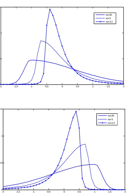
andtα is the 100α% quantile of the standardized Student-ν density. As an illustration,

Figure 2.1 plots the skewed-Student distribution for different degrees of freedom and asymmetry parameterξ= 0.75,−0.75.For small values of ν the density is more peaked and it becomes flatter as long as it increases.

Another asymmetric distribution is the skewed-generalized-t (SGT) distribution pro-posed by Theodossiou (1998). The SGT distribution has the attractive of encompassing most of the distributions usually assumed for standardized returns. For example, the Normal, GED, Student-ν and skewed-Student-ν distributions can be obtained as par-ticular cases. However, in our experience, the maximization of the log-likelihood based on a SGT distribution is very complicated. Consequently, we will not consider fur-ther this distribution; see Bali and Theodossiou (2007) for an application of the SGT distribution in the estimation of theV aR.

Alternatively, instead of assuming a particular distribution of t, several authors

propose to estimate directly qα. For example, Danielsson and de Vries (2000) and

Mc-Neil and Frey (2000) among others, use Extreme Value Theory (EV T) for the tails of the distribution of the standardized residuals; see Chan and Gray (2009) for a nice description of EV T and its application to estimate the V aR of daily electricity prices. This procedure is based on taking into account that, when the conditional mean and variance are correctly specified, the standardized residuals,_bt=

Rt−µbt

b

σt

are iid.Then, they can be used to build the distribution function of the tail. If F is the

(27)

distribu-2.2. Estimation and testing of Value at Risk (V aR) 26

tion of standardized returns, the excess distribution above the threshold u is given by

Fu(y) = P[bt−u≤y |bt> u] =

F (y+u)−F (u)

1−F (u) . Therefore,

1−F (_bt) = (1−F (u)) (1−Fu(bt−u)). (2.7)

The function (1−F(u)) can be estimated by the proportion of observations over the threshold, i.e. by N/T, where N is the number of observations in the sample that exceed u. On the other hand, 1−Fu(bt−u) can be estimated by ML by assuming

that the excess residuals over the threshold have, for example, a Generalized Pareto distribution (GP D) given by

Gξ,β(y) =

1−(1 +ξy/β)−1/ξ if ξ 6= 0 1−exp (−y/β) if ξ= 0

where β is the scale parameter, ξ is the shape parameter such that if ξ >0 the distri-bution has heavy tails. The corresponding probability density function is given by

gξ,β(y) = 1 β 1 + ξy β − 1 +ξ ξ .

In practice, we fix the number of observations in the tail to beN =k, wherek << T,

obtaining a threshold at the (k+ 1)th order statistic. Consequently, if _b(1) ≥...≥b(T)

are the ordered standardized residuals, the threshold is _b(k+1) and the GPD is fitted

to _b(1)−b(k+1), ...,b(k)−b(k+1)

. Using (2.7) we get the following tail estimator for

bt>b(k+1) b F(_bt) = 1− k T 1 +ξbb t−b(k+1) b β −1/ξb . (2.8) Finally, if α < k

T,the quantile can be obtained from (2.8) as follows

b qα =− b(k+1)+ b β b ξ α k/T −ξb −1 !! . (2.9)

The use of the GP D for the excess residuals is just an example of a heavy-tailed distribution. Gnedenko (1943) characterizes all such distributions by the following formula for x > u

(28)

Applying expression (2.10) to the ordered residuals beyond the (k+ 1)th order statistic and choosing L(_b) = k

T b(k+1)

1/ξ

, the following tail distribution is obtained

F (_bt) = 1− k T bt b(k+1) −1/ξ . (2.11)

In this case, the shape parameter ξ can be estimated using the estimator proposed by Hill (1975) that is given by

b ξ(H) = 1 k k X j=1 log _b(k) −log _b(k+1) . (2.12)

The estimation of the quantile is then

b qα =−b(k+1) α k/T −ξb(H) . (2.13)

One important issue related with the Hill estimator is the choice of the number of observations in the tail, k. In this sense, McNeil and Frey (2000) show that the

EV T method based on the GP D distribution gives more stable quantile estimates than the Hill estimator. To illustrate this point, the quantile is obtained by the Hill estimator and the GP D distribution using the procedure explained above. Figure 2.2 plots Hill estimates of the 1% quantile of the returns of the S&P500 index observed from 29/08/1995 to 20/10/2005 for different values of k. This figure shows that, as expected, the Hill estimator of q0.99 is an increasing function of k, although it is very

unstable when the number of observations over the threshold is small. This figure also plots the estimates based on the GP D distribution which are also very unstable for small k.However, whenk > 30, the estimate of q0.99 is approximately 2.6 regardless of k. Note that the same estimate is obtained by the Hill estimator when 30< k < 250.

Only for very large values of k the Hill estimator generates estimates ofq0.99 well over

2.6. Therefore, if the number of observations in the tail is moderate, i.e. between 30 and 250, both estimators should give the same answer. It is clear that the choice of the threshold is an important issue in EV T since it may have severe consequences on the tail estimates. Danielsson and de Vries (1997) and Danielsson et al. (2001) have developed bootstrap methods for optimal threshold selection in the context of the Hill estimator. However, the selection of the threshold using bootstrap procedures is

(29)

very time consuming. Alternatively, Gonzalo and Olmo (2004) propose a single step approach to threshold selection.

Chan et al. (2007) derive the asymptotic distribution of the quantile estimator of McNeil and Frey (2000) in (2.9) without assuming a specific parametric distributional assumption on the heavy tailed distribution of t. Then, they propose two alternative

methods to construct confidence intervals of the V aR. The first method is the tradi-tional method based on the asymptotic Normality of theV aRestimator. Alternatively, they propose to construct confidence intervals by the tilting method of Hall and Yao (2003) and Peng and Qi (2003). Note, that the confidence intervals for the V aR con-structed in this way do not incorporate the uncertainty due to the estimation of the parameters of the conditional mean and standard deviation.

Alternatively, the quantileqα can be estimated using bootstrap methods that do not

assume any particular distribution of the errors and incorporate the uncertainty of the estimated parameters; see Ruiz and Pascual (2002b) for a review of the literature on using bootstrap procedures in financial time series and, in particular, for the estimation of the V aR. In particular, Hull and White (1998) and Barone-Adesi et al. (1999) propose a bootstrap method called Filtered Historical Simulation (F HS) based on using random draws with replacement from the standardized residuals. Bootstrap procedures have the advantage of allowing to obtain confidence intervals for the estimated V aR. For example, Christoffersen and GonC¸ alves (2005) implement the bootstrap procedures proposed by Pascual et al. (2006) to obtain confidence intervals for the V aR that incorporate the parameter uncertainty. They show that the confidence intervals for

HS are too narrow and do not contain the true V aR with the desire frequency while the methods that properly account for conditional variance dynamics imply confidence intervals with coverages close to the nominal. Bootstrap procedures have also been implemented by Hartz and Paolella (2006) who additionally propose a bias-correction method for improving theV aRforecasting ability of the GARCH model withN ormal

errors (GARCH −N).

The procedures described up to now are based on assuming a parametric specifi-cation of the conditional mean and variance. However, semiparametric and

(30)

nonpara-2.2. Estimation and testing of Value at Risk (V aR) 29

metric specifications have also been considered in the literature. For example, Fan and Gu (2003) introduce a semiparametric model to estimate the volatility using the geo-metric Brownian motion, a time-dependent diffusion model, as a discretization of the

IGARCH(1,1) model of Riskmetrics. In order to estimate the decay factor needed

for the Riskmetrics methodology they propose two alternatives, one resulting in a data dependent decay factor which remains constant in the forecasting period, and the other which adapts automatically to changes in stock price dynamics, adding flexibility to the first decay factor. Additionally, Fan and Gu (2003) propose a symmetric nonpara-metric estimation approach to estimate the quantiles of the standardized residuals. On the other hand, Martins-Filho and Yao (2006), based on the two stage approach of McNeil and Frey (2000), propose a nonparametric estimation procedure for the condi-tional mean and variance using the local linear estimator of Fan (1992). Furthermore, they propose a method based on L-Moment theory instead of the GP D used by Mc-Neil and Frey (2000). These nonparametric methods are more difficult to implement than the parametric procedures. However, inferential gains can be obtained when the assumptions of the parametric models are wrong. Another nonparametric procedure is that developed by Chen and Tang (2005b). They propose to calculate the V aR by implementing kernel smoothing on the empirical distribution of returns in such a way that the estimator of theV aRis a weighted average of the order statistics aroundRω:T.

They also emphasize the importance of the standard error of the V aR estimates and develop a procedure for its estimation based on a kernel estimation of the spectral den-sity function of a series built using the smoother function. More recently, Cai and Wang (2008) developed a nonparametric estimator of the V aR and the ES by obtaining a weighted double kernel local linear estimator of the conditional distribution function. The proposed estimator is a combination of the weighted Nadaraya-Watson method of Cai (2002) and the double kernel local linear method of Yu and Jones (1998).

Finally, there is another alternative to estimate the V aR by modeling directly the dynamic evolution of the quantiles over time. The Conditional Autoregressive Value at Risk (CAV iaR) was introduced by Engle and Manganelli (2004) who propose the

(31)

following equation for the V aR

V aRα_t =β0+β1V aRαt−1+l β2, Rt−1, V aRαt−1

(2.14)

where different forms of the function l can be proposed. Some examples are the asymmetric slope, l(·) = β2(Rt−1)++β3(Rt−1)

−

, where (x)+ = max (x,0), (x)− =

−min (x,0),and the adaptive,l(·) = β2 n

1 + exp GRt−1+V aRtα−1

−1

−αo, where G is some positive finite number. The parameters of this model are estimated by the method of regression quantiles developed by Koenker and Bassett (1978). Manganelli and Engle (2001) also incorporate EV T to CAV iaR. The procedure is the follow-ing: first, fit a CAV iaR model to get an estimation of the V aR for a large α, for example 10%, then construct the series of standardized quantile residuals as follows:

b t,α [ V aRα_t = Rt [ V aRα_t !

−1 and apply EV T to this series to get an estimation of the tail

b

qp forp < α. Then, the V aRis calculated as

[

V aRp_t =V aR[α_t (1 +q_bp). (2.15)

Alternatively, DeRossi and Harvey (2006) propose to combine the approach of Engle and Manganelli (2004) with signal extraction. The idea is to use some of the forms of the functionland approximate them to the filtered estimators of time-varying quantiles. Recently, Gourieroux and Jasiak (2006) proposed a dynamic adaptive quantile which improves the approach of Engle and Manganelli (2004) by taking into account the monotonicity of quantile estimators which ensures that the quantile is an increasing function of α. On the other hand, Chen and Chen (2005) compare the performance of the Riskmetrics approach and theGARCH(1,1)−N andGARCH(1,1)−t models for estimatingV aRwith the combination of them with quantile regression. They conclude that the quantile regression combined with the GARCH(1,1)−t provides the best estimates.

(32)

2.2.2 Backtesting VaR estimates

In order to asses the accuracy of V aR estimates, the Basel Committee on Banking Supervision (1996b) and the amendments of Basel Committee on Banking Supervision (1996a) develop a statistical testing device denominated backtesting. According to their requirements, the backtesting should be based on 250 one step-ahead estimates of the V aR, i.e. estimates over one year. In this section, we review the most popular backtesting procedures proposed in the literature. Backtesting is based on testing whether theV aRestimates are statistically accurate. When there are several alternative estimators of theV aR, one may additionally want to choose the best among those that generate accurate estimates; see, for example, Sarma et al. (2003) and Angelidis and Degiannakis (2007).

Backtesting procedures are based on the failure process I_tα = 1 (Rt<−V aRtα),

t=T+ 1, ...T+n,where 1 (·) is the indicator function, T is the size of the sample used

to estimate theV aR and n is the number of one step-ahead V aR’s computed. A V aR

estimator is accurate if and only if

E t−1[I

α

t] =α. (2.16)

Most backtesting procedures are based on testing some of the implications of this condition. The most popular backtesting procedure, proposed by Kupiec (1995), is based on the number of failures defined asx=

T+n

P

T+1

Iα

t which has a binomial distribution

with parameters n and α. Kupiec (1995) proposes to test the null hypothesis H0 : E[I_tα] =α, using the following likelihood ratio statistic

LRuc= 2 log 1− x n n−xx n x −2 log(1−α)n−xαx. (2.17)

Under the null, the LRuc statistic has asymptotically a χ2₍₁₎ distribution. It has low

power when implemented with small samples. However, note that the null hypothesis is testing whether the unconditional expectation is α, which is not the hypothesis of interest in (2.16). Consequently, Christoffersen (1998) proposes a test of conditional coverage, where the null hypothesis is given byH0 :E

Iα

t |Itα−1

(33)

to testing whether Iα

t are iid Ber(α) random variables against the alternative of first

order Markov dependence. Note that this condition is necessary but not sufficient for the hypothesis in (2.16). This test considers whether the unconditional coverage is correct and adds a term to consider the serial independence of the failure process{It}.

The serial independence term,LRind, is defined as follows

LRind= 2 log [(1−π01) n00 πn01 01 (1−π11) n10 πn11 11 ]−2 log (1−π)n00+n10 πn01n11 _(2.18)

wherenij is the number ofItα observations with valueifollowed by an observation with

value j, for i, j = 0,1 and π01 = _n n01

00+n01, π11 =

n11

n10+n11. Under the null hypothesis

π01 = π11 = π = n01+_nn11 and the LRind statistic has an asymptotic χ2₍₁₎ distribution.

Finally, the likelihood ratio for conditional coverage,LRcc is defined as

LRcc =LRuc+LRind (2.19)

which has asymptotically a χ2

(2) distribution under the null.

Recently, other tests for independence based on the autocovariances Cov Iα t, Itα−j

have been proposed. For example, Berkowitz et al. (2006) discuss the following Port-manteau test LB(m) = (n) (n+ 2) m X j=1 (n−j)−1r_j2 (2.20)

where rj is the order j sample autocorrelation of Itα − α. Under the null, LB(m)

is asymptotically χ2

(m). On the other hand, Engle and Manganelli (2004) suggest a

dynamic quantile (DQ) test obtained by regressing I_tα−α against its lagged variables and other values included in the conditioning set and testing whether these variables are significant.

The backtesting tests described above are based on the assumption that the param-eters of the models fitted to estimate the V aR are known. However, in practice, these parameters have to be estimated. Escanciano and Olmo (2010) show that the use of standard unconditional and independence backtesting procedures to assesV aRmodels in out-of-sample environments can be misleading. They quantify the risk associated with the estimation of the parameters in a very general class of dynamic parametric

(34)

V aRmodels and propose a correction of the standard backtesting procedures that takes into account such a risk. They show that one of the main determinants of the corrected asymptotic variance is the forecasting scheme used to generate the forecasts of theV aR, i.e. whether one uses recursive, rolling or fix parameter estimates.

The backtesting procedures help to decide whether a particular procedure gives accurate estimates of theV aR. However, when several accurate estimators are available, one wants also to decide which estimator is best among them. With this goal, Lopez (1999) proposes to choose the procedure that minimizesCm =

PT+n t=T+1Cm,t where Cm,t = f Rt, V aRαm,t if Rt< V aRαm,t, g Rt, V aRαm,t if Rt≥V aRαm,t.

where the index m is used to represent the procedure m to estimate the V aR and

f(x, y) and g(x, y) are functions such that f(x, y)≥g(x, y).

Different loss functions has been proposed in the literature; see Lopez (1999). Sarma et al. (2003) and Angelidis and Degiannakis (2007) use the following Regulatory Loss function (RLF) that is similar to the Quadratic Loss Function proposed by Lopez (1999) Cm,t = Rt−V aRαm,t 2 if Rt< V aRαm,t, 0 if Rt≥V aRαm,t. (2.21)

Angelidis et al. (2005) proposed the Quantile Loss function (QLF) that additionally penalizes for higher than needed amount of capital. It is defined by

Cm,t = ( Rt−V aRαm,t 2 if Rt< V aRm,tα , Rω:n−V aRαm,t 2 if Rt ≥V aRαm,t. (2.22)

On the other hand, Giacomini and Komunjer (2005) and Bao et al. (2006) compare competingV aRforecasts using the predictive quantile loss function (P QLF) based on the methodology of Koenker and Bassett (1978). TheP QLF function is given by

Cm,t = [α−1 (Rt< V aRtα)] [Rt−V aRαt]. (2.23)

Alternatively, when trying to establish the superiority between two models Sarma et al. (2003) propose the following testing procedure

(35)

H0 :{θ = 0} vs H1 :{θ < 0}

where θ is the median of the distribution of the loss differential between procedure

i and procedure j, zt = Ci,t − Cj,t. The number of non-negative z0s is defined as

Sij =

PT+n

t=T+1ψt, whereψt= 1 (zt≥0). Under the null hypothesis, the exact

distribu-tion ofSij is binomial with parameters (n,0.5) and the asymptotic distribution of the

standardizedSij is given by Sij −0.5n √ 0.25n a ∼N(0,1) ; (2.24)

see Diebold and Mariano (1995). If H0 is rejected, model i is significantly better than

model j for the chosen loss function. Note that the statistic in (2.24) can be obtained as the t-statistic of the regression ofzt on a constant using the Newey and West (1987)

heteroscedasticity autocorrelation consistent (HAC) standard errors.

An alternative to the test in (2.24) is the test of conditional predictive ability, proposed by Giacomini and White (2006), which takes into account the estimation uncertainty due to model selection. The one-step-ahead conditional predictive ability statistic is given by CP AT ,n=n n−1 T+n−1 X t=T ht∆Cm,t+1 !0 b Ω−_n1 n−1 T+n−1 X t=T ht∆Cm,t+1 ! , (2.25)

whereΩb_n is a consistent estimate of the variance of h_t∆C_m,t₊₁ and h_t is a q×1 vector

given byht= (1,∆Cm,t)

0

. The null hypothesis of equal conditional predictive ability is rejected whenCP AT ,n > χ2q.

On the other hand, Angelidis and Degiannakis (2007) and Bao et al. (2006) propose to compare alternative models using the test of superior predictive ability (SP A) of Hansen (2005). The null hypothesis, that the benchmark model (m= 0) is not inferior than the alternatives, is tested with the following statistic

T_nSP A= max max m=1,...,M n1/2_z m b ωm ,0 , (2.26) where _bω2

m is a consistent estimator of ωm2 = var n1/2zm

, zm = n−1

Pn

t=1zm,t and

(36)

2.3. Estimation and testing of Expected Shortfall (ES) 35

using the stationary bootstrap of Politis and Romano (1994) with the optimal block-size chosen by the block selection algorithm proposed by Politis and White (2004).

Finally, Giacomini and Komunjer (2005) propose to compare two V aR forecasts versus its combination using a conditional quantile forecast encompassing test of su-perior predictive ability. A rejection of the test provides statistical evidence that the combination outperforms the two individual forecasts.

2.3 Estimation and testing of Expected Shortfall

(

ES

)

This section describes different methods proposed in the literature for estimating ES.

As we mentioned above,ES is a relatively new measure of risk, and consequently there are fewer papers dealing with its estimation. Most of the papers actually estimate

CV aRinstead ofES. Remember that theCV aRonly is coherent if the returns have a

continuous probability distribution but, in practice, the distribution of returns is often assumed to be continuous and, in this case, the CV aRand the ES are equivalent. We also describe methods to evaluate the accuracy of the estimatedES.

2.3.1 Estimation

Acerbi and Tasche (2002) propose to estimate the ES using the V aR estimator based on Historical Simulation. In this case, the estimator is given by

c

ESα_t =R(ω), (2.27)

where R(ω) =

Pω

i=1Ri:T

ω is the average of the smallest 100α% returns. This estimator

has a positive bias attributable to the negative biases of the order statistics. Conse-quently, Inui and Kijima (2005) has proposed an extrapolation method to adjust the bias and stabilize the estimator.

Alternatively, several authors propose to estimate theES as the average of observed returns beyond the V aR when the V aR has been estimated by one of the methods

(37)

described in the previous section; see, for example, Giot and Laurent (2003) and Bali and Theodossiou (2007).

On the other hand, instead of using the sample mean of the returns beyond the

V aR, note that if returns are given by equation (2.1) then the ES is given by

ES_tα =µt+σtE

t−1[t|t ≤qα]. (2.28)

There are different alternative methods proposed to calculate E

t−1[t|t ≤qα]. First,

one can assume a particular distribution for the innovations and calculate analytically the corresponding expectation. If, for example, they are Normal, then E[t|t ≤qα] =

−φ(Φ

−1

α )

α , where Φ

−1

α is the αth quantile of the standard Normal distribution. On the

other hand, if the innovations are Student-ν,then

E[t|t≤qα] = ν−2 α(1−ν) Γ ν+ 1 2 r π(ν−2) Γν 2 1 + q 2 α ν−2 1−ν 2

where qα is the αth quantile of the standardized Student-ν; see Christoffersen and

GonC¸ alves (2005) for an empirical application. In the case of theGED and the Skewed-t disSkewed-tribuSkewed-tions, Skewed-the corresponding condiSkewed-tional expecSkewed-taSkewed-tions can be esSkewed-timaSkewed-ted by MonSkewed-te Carlo simulations.

Another procedure to estimate the ES is by using EV T in order to estimate the tail of the distribution of the standardized residuals and then, calculate the conditional expectation of the values beyond the quantile qα; see McNeil and Frey (2000). In

this case, if the excess residuals over the threshold u are assumed to follow a GP D

distribution with parameters ξ < 1 and β, then the expected shortfall is estimated as follows c ESα_t₊₁ =µ_bt+1+bσt+1qbα   1 1−ξb + βb−ξb(k+1) 1−ξb b qα  . (2.29)

Alternatively, using the Hill estimator we can obtain the following estimation of the

ES c ESα_t₊₁ =_bµt+1+σbt+1 b qα 1−ξb(H) . (2.30)

(38)

Another method for estimatingES isF HS as in Giannopoulos and Tunaru (2005). Once the bootstrap distribution of returns is obtained, the ES estimator is calculated as the sample average of the returns that exceedV aR. We can also obtain the bootstrap distribution of returns using the procedure develop by Pascual et al. (2006) and then estimate the ES as the average of the returns that exceed V aR. Christoffersen and GonC¸ alves (2005) implement the bootstrap procedure of Pascual et al. (2006) to obtain confidence intervals for alternative estimators of theES. They show thatES measures are generally less accurate than V aR measures and that the confidence bands around

ES are also less reliable. Table 2.2 contains a summary of different assumptions onµt, σt and the distribution of t proposed in the literature for estimating the ES.

2.3.2 Backtesting ES estimates

In order to evaluate the adequacy of the estimated ES, Angelidis and Degiannakis (2007) propose a two steps evaluation framework that extends the evaluation approach of Lopez (1999). In the first step, the correct conditional coverage of theV aR forecast is tested using theLRcc statistic in equation (2.19). In the second step, the loss function

is calculated with respect to the ES instead of the V aR, because the V aR does not give information about the size of the expected loss. The loss function is then

Cm,t = Rt−ESm,tα 2 if Rt < V aRαt 0 if Rt≥V aRαt , (2.31)

where the subindex m refers to model m. For each model, the mean squared error is calculated byM SE = 1

n

PT+n

t=T+1Cm,t. We choose the model that minimizes theM SE.

However, in this case, there is some ambiguity about the interpretation of theM SE.

In order to overcome this problem, alternative models can be tested by using the test of superior predictive ability of Hansen (2005). Note that this procedure tests for superiority among the models that provide accurate V aR forecasts, but it is not a method to test the accuracy of the ES forecasts.