From Clouds to Planet Systems Formation and Evolution of Stars and Planets

From Clouds to Planet Systems

Formation and Evolution of Stars and Planets

G¨unther Wuchterl

June 13, 2005

Abstract

The discovery of more than hundred extrasolar planet candidates chal-lenges our understanding of star and planet formation. Do we have to modify the theories that were mostly developed for the solar system in or-der to unor-derstand giant planets orbiting their host stars with periods of a few days? Or do we have to assume particular circumstances for the for-mation of the Sun to understand the special properties of the solar system planets? I will review the theories of star and planet formation and outline processes that may be responsible for the diversity of planetary systems in general. I will discuss two questions raised by extrasolar planets: (1) the formation of Pegasi-planets and (2) the relation between discovered extra-solar planets and the metallicity of their host stars. Finally I will discuss the role of migration in planet formation and describe three tests in or-der to distinguish whether planets migrated long distances or formed near their final orbits.

1

Witnessing the Discovery

What happened to the theory of star and planet formation, when almost ten years ago, in October 1995, Mayor and Queloz (1995) announced that they had found a planet, in a 4 day orbit around the 5th magnitude star 51 Pegasi? Theory at this time was preparing for the discovery of extrasolar planets in orbits around common, main-sequence stars. Yet the first discoveries seemed to be well in the future, not to be expected before the start of the new, the third millennium.

1.1

Observations: 12 years, 21 stars - no planet (yet)

In August that year, planet searchers from the University of British Columbia, led by Gordon Walker, had published their 12 year long effort to monitor 21

∗_{Astrophysikalisches Institut und Universit¨ats-Sternwarte Jena, Schillerg¨aßchen 2, D–} 07745 Jena, Germanyhttp://www.astro.uni-jena.de/wuchterl

solar-like stars for planetary companions. It was widely considered the first search having the required sensitivity to detect planets. And as everybody considered self-evident, the easiest one to detect would be a Jupiter-like planet in a Jupiter-like orbit of approximately 12 years period. After all that was the case for the solar system put to 10 parsec, the typical distance of a nearby star. When Walker et al. (1995) published that they had not found any planet1

and gave an upper limit of less then 1 in 10 stars having a ‘Jupiter’, the formation theorists started to wonder about the result. It was generally considered that solar system formation theory was not yet complete. But should the solar system be more special after all, then the Sun was compared to other stars? I.e. a typical member of the galactic minority of single stars that is outnumbered by a factor of about 3 by stars that are in multiple systems.

The Wolszczan and Frail (1992) finding of planets in orbit around the Pulsar PSR-B1257+12, had been confirmed by Wolszczan (1994) using modifications of the planetary orbits by mutual perturbations of the inferred planets them-selves. Hence apparently planet formation was a rather ubiquitous process also occurring in one of the very exotic environments that the millisecond pulsar had provided during its long history.

1.2

Theory: not quite in place

That October theorists had assembled on the Island of Hawaii to discuss extra-solar planets and their formation. The discovery seemed like a reality shock. I still remember the faces of other theorists after the message of the discovery of 51 Pegasi was put on an overhead projector at the end of the extrasolar planets session. We realised that we were on the wrong side of the globe. The discovery was announced in Florence, close to Galileo’s last home. Theory was taken by surprise. A ‘Jupiter’ at 1/100 of Jupiter’s orbit, a few stellar radii from its host star was a bewildering thing. It was not that anyone had proven or even tried to prove that giant planets could not form close to their stars. Apparently nobody had even thought about it. Everybody wondered how this could have happened and there was at the same time concentrated thinking: how could it form? I am sure, that as we travelled home we all had an idea how to make it. When I stepped out of the plane in Frankfurt, I had convinced myself that it actually would be easy to form 51 Peg’s planet and planned the calculations to prove that. Similar events must have happened for many people because within a year many ideas for the formation of 51 Pegasi b were published.

I am telling this because it is exciting and also because it helps to under-stand the diversity of ideas that developed after the discovery of 51 Pegasi b. Before that, there was a fairly detailed framework for the understanding of the formation of the solar system. It was a step-wide approach, tied into the data from the history of the solar system. Supposedly it could be generalised to other

1_{AlthoughγCep was a special case where the planetary interpretation could not be rejected} with certainty, cf. Walker et al. (1992). In the meantime two of the stars of Gordon Walker’s list are known to host planets: ²Eridani Hatzes et al. (2000) andγCephe¨ı A Hatzes et al. (2003). Twelve years of data were not enough.

systems. But it had and has its open questions. Hence research focused on clos-ing the holes for the solar system where the data was rich. An understandclos-ing of a general theory of planet formation was only beginning. As the pioneering work for understanding planet formation around stars of various masses I rec-ommend a series of three papers: Nakano (1987, 1988a,b). Nakano discusses the limitations for planet formation based on growth time-scales and nebula and stellar lifetime in the framework of theKyoto-model.

Just before the discovery Jack Lissauer gave a talk on theDiversity of plau-sible planetary SystemsLissauer (1995). It is a careful assessment and weighting of the uncertainties trying to focus on what can be expected for other systems from what we have learned for the solar system. I think every person interested in what could be expected from theory will find the overview there.

2

Planet Formation Theory

2.1

The ‘Original’ Solar System Perspective

So there is the classical picture based on the formation of the solar system until 1995 and the diversity of ideas thereafter, with a manifold of scenarios for planet formation. Many of them probably inconsistent with solar system formation or of unknown relation to the solar system.

To get an overview over the classical picture of solar system formation, I recommend the review article of Hayashi’s Kyoto-group Hayashi et al. (1985), where the stage is set for modern theories2_{— planets forming in a circumstellar,}

protoplanetary disk of gas and dust, that originates from an interstellar cloud together with the host (proto)-star. The article discusses the key physical pro-cesses and outlines a complete picture of solar system formation. The overall picture is basically unchanged up to now, but some of the numbers have been corrected and gaps in the argumentation have been closed. To get a more quan-titative view, especially on terrestrial planet formation and a concept to resolve the issue of the long growth time of the cores of giant planets I recommend Jack Lissauers Lissauer (1993) article onPlanet Formation inAnnual Reviews of Astronomy and Astrophsics. It is written after a half-year long get-together of essentially all researchers on planet formation in 1992, at Santa Barbara. It is a superb review and covers the situation of planet formation theory at that pre-51 Peg-time.

2_{v. Weizs¨acker Weizs¨acker (1943) distinguishes three mayor groups of planet formation} theories: A. planets formed from a uniformly rotating mass, that filled the space of the present planetary system (Kant, Laplace). B. Planets formed from a tidal-wave [Flutwelle] that was excited by a star passing the Sun (Chamberlin, Moulton). C. Planets formed from an irregularly shaped nebula-filament (N¨olke). I consider work following thenebula hypothesis (A.) supplemented by theplanetesimal hypothesisas modern formation theories

2.2

After 51 Pegasi — Forget the Solar system?

With the ‘discovery shock’ many researches apparently felt that the solar system approach was ‘dead’ and invented numerous schemes to rapidly explain the new object. A year after the discovery it was still a close race between the number of discovered planets and the number of new theories to explain them.

New processes were invoked — often rather ad hoc — to explain the un-expected properties of 51 Peg as well as the growing diversity in the observed exoplanet population. Some of the new processes apparently played no or only a minor role in the solar system. The unpredicted properties of extrasolar planets — giant planets in orbits with periods of a few days, eccentricities much larger then any of the Sun’s planets, and many giant planets with orbital radii much smaller than Jupiter’s — prompted strong comments:

Upon the discoveries, theorists have lost the understanding of the formation of the solar system,

as Pavel Artymovic put it at the IAU symposium 202 at the Manchester general assembly in 2000 or more drastically:

Forget the solar system!,

as a well known astrophysicist recommended off the records in 2002. Are we witnessing that the copernican principle is finally failing in cosmogony? Is the formation of our own home-system fundamentally different from the typical planet formation process in the galaxy? Are special processes or unlikely cir-cumstances required to explain the properties of the Solar System?

3

Introduction - Trying to solve a big problem

The approach I will follow to look at the problem and possibly contribute to answer these questions is not to describe the diversity of theories and ideas but focus on a simplified picture that is closely linked to basic physical principles. Essentially to the equations that describe the fluid-dynamics of a mixture of gas and dust supplemented by the theory of planetesimal growth.

The idea is to provide understanding of a theoretical backbone that is un-likely to suffer refutation, unless one of its key assumptions turns out to be invalid.

Those assumptions are

1. There exists an angular momentum transfer process to separate mass and angular momentum during protostellar collapse,

2. Dust-growth in the protoplanetary nebula leads to km-size planetesimals on a time-scale that is fast compared to nebula-evolution,

3. The basic properties of stars and planets can be described with spherical symmetry.

I will not discuss many results in the literature based on my judgment of how close they are to a deductive, more theoretical physics approach. It is not be-cause they may not be relevant but bebe-cause they are usually snap-shot studies of a particular process without a clear justification of previous or later phases of star and/or planet formation. Often unknown physical processes are param-eterised to make the respective models solve-able.

So I emphasise parts of the problem that can be solved with relatively high reliability but neglect the addition of processes that will occur in reality but can not be reliably quantified. Such, the picture given here will not address many aspects of the problem that are needed to understand all the properties of star planet systems but what is discussed should hold, although it may turn out to be of minor relevance for the big picture.

The analogy for the Sun would be to just discuss the global properties like mass, luminosity, temperature and age but ignore surface effects like spots and other magnetic activity and global effects like differential rotation and globally relevant circulation patterns inside the convection zone and granulation.

4

The Plan

We will start our considerations with interstellar clouds and proceed to planets in three steps:

1. star formation as collapse of a gravitationally unstable cloud fragment, 2. early evolution of the star and a plausible circumstellar, protoplanetary

nebula,

3. planet formation in the protoplanetary nebula.

I will discuss protostellar collapse and early stellar evolution with detailed solutions for the spherical problem for masses down to the brown dwarf regime. This is analogous to describing stellar evolution to and from the main sequence, with the important difference that due to the collapse-origin of stars fluid dy-namical processes are important. Accretion-flows determine the luminosity, structure and evolution during the earliest phases that last approximately a Ma (1 Ma = 1 Million years).

A similar first principles approach is presently not feasible for the formation of the protoplanetary nebula. Hence I will briefly describe the ongoing efforts and the fall back to a pragmatic approach to construct plausible protoplanetary nebulae for planet formation studies. The resulting models then give estimates for the nebulae conditions that then can be used as starting point for the con-struction of planet formation models.

In the third step, i.e. planet formation I will return to a more basic princi-ple oriented approach. The theory of planetesimal accretion will be combined with spherical models of protoplanets that consist of a core and a gaseous en-velope that are embedded in a plausible protoplanetary nebula. These models will provide masses, luminosities and accretion-histories for planets. Finally I

will discuss some applications, including observational test of planet formation theory.

For convenience and consistency I will mostly use my own models that are applicable to stars, brown dwarfs and planets and are based on the same set of basic physical equations and identical descriptions of the microphysics. They all use the sameconstitutive relations, i.e. equations of state and opacities. The sys-tem of equations is calibrated to the Sun and observationally tested by the solar convection zone and RR-Lyrae light-curves Wuchterl and Feuchtinger (1998); Wuchterl and Tscharnuter (2003).

5

From Clouds to Stars

5.1

Clouds

Stars form from molecular clouds. Most of the clouds’ mass is in molecular hydrogen. Some of them can be seen as nearby dark clouds because the dust they contain obscures the light of milky-way stars behind them. In some of the dark clouds faint stars can be seen that have ages of a few Mio years. These

T-Tauristars have not yet ignited hydrogen burning and will evolve towards the main sequence in a few 10 Ma. Hence this evolutionary phase is often referred to as the pre-main sequence phase. Only when their nuclear reactions will produce energy with a sufficient rate to balance the energy that is radiated from their surfaces, the process of gravitational contraction stops. Once that balance is reached typical stars will stay on the main sequence with approximately constant luminosity and surface temperature for∼109_years.

Star formation preferentially occurs in the spirals arms of the galaxy. Gi-ant molecular clouds there have masses of 1 Mio solar masses and fragment into substructures that finally lead to the sub-collapses of sub-fragments, that typically result in a cluster of stars. Star formation is a multiple scale process reaching from sizes of 100 pc clouds with subunits referred to as clumps down to smallest structures termed cores of 0.1 pc and masses comparable to the stellar ones, i.e. of typically a solar mass. Galactic tides, magnetic fields and irregular motion (turbulence) play a role on larger scales but ultimately star formation is a competition between the support by thermal pressure and the inward pull of gravity. Once gravitational collapse starts and the cloud-cores shrink, rotation becomes more and more important. As the sizes shrink, conservation of angular momentum leads to a spin up even for initially slow rotating structures. The common outcome are clusters of stars, multiple systems and star-disk systems. That way the classical angular momentum problem — even a slowly rotating cloud would lead to a hypothetical stellar embryo rotating much faster than breakup speed — is most likely solved by redistribution of angular momentum between the components.

I focus on the physics of star formation that is most relevant for planet formation. That is most importantly the properties of the new-born protostar and the protoplanetary nebula as well as the time-scales for the final collapse

and early stellar evolution. A general review of thephysics of star formationhas recently given by Larson (2003). Two stages of cloud collapse may be discerned:

1. fragmentation of the cloud,

2. collapse and accretion of cloud fragments.

Instead of discussing the fragmentation process of molecular clouds I will assume that it leads to fragments of all masses down to the opacity limit of fragmen-tation, which is estimated to be at approximately 0.01 – 0.007 MSunor 7–10

MJupiter3. Below the opacity limit further fragmentation into still smaller mass

units is likely made more difficult or impossible. That is due to the tempera-ture increase which is a consequence of the dense fragments becoming opaque for light of all wavelengths that are capable to carry out energy and hence cool the collapsing clouds that are heated by gravitational self-compression. Indeed stars may have their masses determined directly by those of the prestellar cloud cores. That is suggested by the fact that the distribution of masses or ‘initial mass function’ (IMF) with which stars are formed appears to resemble the dis-tribution of masses of the prestellar cores in molecular clouds (Larson (2003), for discussion).

To determine the physical properties of the final fragments, that just became gravitationally unstable, we consider the balance of gravity and thermal pressure in a cloud-core of given temperature,T and mass-density (or density for short)

%. Such a fragment is unstable to perturbations, i.e. density fluctuations, if its size is or volume contains a mass that is larger than theJeans-mass:

MJeans=ρλ3Jeans, (1)

with theJeans-length,

λ3

Jeans=cT r

π

G% (2)

whereG is the gravitational constant,cT = p

P/%=pkT /m, the isothermal sound speed for an ideal gas of particles with mean massm, with the Boltzman constant k. The other constant factors depend somewhat on the details of the assumed geometry of the cloud and the perturbations respectively density fluctuations assumed in the cloud4_.

We will restrict our discussion of formation to the discussion of star-formation from gravitationally unstable — to be more specific Jeans-unstable — cloud cores as an idealisation of the smallest cloud fragments. To be more precise we will mostly discuss star formation from cloud fragments that are actual

3_{1 M}

Sun= 1.989 1030kg,1 MJupiter= 1.899 1025kg,1 MEarth= 5.974 1024kg, 1 MJupiter= 0.95 10−3_M

Sun,1 MJupiter = 317.8 MEarth. I will use 0.001 MSun and MJupiter as approxi-mately equal.

4_{Planar waves are used in the case given. A discussion of variants of the Jeans instability} and more rigourous treatments that avoid theJeans-swindleof assuming an unperturbed state that is not an equilibrium solution is given in Larson (2003) or text-books as Kippenhahn and Weigert (1990)

rigourous solutions for the equilibria of self-gravitating isothermal clouds with spherical symmetry that are embedded into a medium of finite, constant pressure (the ambient larger cloud superstructure). Such self-gravitating equilibrium gas-spheres are called Bonnor-Ebert-gas-spheres, Bonnor (1956); Ebert (1957). Such theoretical constructs do actually exist in the sky: the structure of a relatively nearby dark-cloud, the Bok-globule Barnard 68, has been found to closely match a Bonnor-Ebert sphere, Alves et al. (2001).

The neglect of rotation, magnetic fields and turbulence as well as the use of spherical symmetry, that lead to the classical Jeans-picture with thermal pressure and gravity as the only players, may seem somewhat restrictive, but we follow Larson (2003) in noting that

... the Jeans length and mass are still approximately valid even for configurations that are partly supported by rotation or magnetic fields, as long as instability is not completely suppressed by these effects. Thus, if gravity is strong enough to cause collapse to occur, the minimum scale on which it can occur is always approximately the Jeans scale, and structure is predicted to grow most rapidly on scales about twice the Jeans scale.

5.2

Clouds and Stars

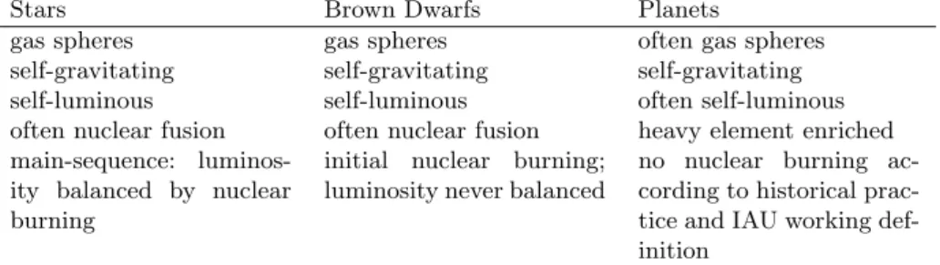
We have looked at the clouds in the beginning. Let us now look at the outcome of the formation process, the products of the cloud collapse: stars, brown dwarfs and planets, that we will refer to ascelestial bodies for short. Basic properties that emphasise similarities are summarised in Tab. 1. What are the common

Stars Brown Dwarfs Planets

gas spheres gas spheres often gas spheres

self-gravitating self-gravitating self-gravitating self-luminous self-luminous often self-luminous often nuclear fusion often nuclear fusion heavy element enriched main-sequence:

luminos-ity balanced by nuclear burning

initial nuclear burning; luminosity never balanced

no nuclear burning ac-cording to historical prac-tice and IAU working def-inition

Table 1: Basic properties of stars, brown dwarfs and planets.

physical principles of these celestial bodies? Arguable the most important one that distinguishes them from other common objects in the universe like rocks, plants, animals and cars is the importance of gravity. Newtonian gravity is described by the Poisson-equation, that in spherical symmetry can be integrated once and written in the form:

dMr

dr = 4πr

where % is the density and the mass interior to radius r for a radial density distribution%(r) is obtained by the integration mentioned above as:

Mr=

Z _r 0

4πr02%dr0. (4)

The corresponding gravitational force that acts on the structure at distancer

is:

Fgrav=−GMr

r2 % . (5)

This leads us to one of the most important principles of astrophysics, namely the force-balance between gravity and pressure(-gradients) that governs the struc-ture of gravitating gas-spheres throughout most of their life, namely hydrostatic equilibrium:

dP

dr =Fgrav=−

GMr

r2 % . (6)

Pressure has entered the considerations and hence we have to specify an equation of state that relates pressure and density. For fully degenerate objects, as white dwarfs and neutron stars, and to some extent for planets, when they behave as liquids, the dominating pressure dependence is on density. Then our equations for the structure would be completed by specifying the pressure as a function of density alone. In general, however, and in any case for high temperatures, the pressure depends on densityand temperature, as, e.g. in an ideal gas with particles of mean massm:

P = %

mkT , often written asP = Rgas

µ %T . (7)

The first version uses the mean particle mass directly and hence the Boltzman constant appears explicitly, the second version uses quantities for a mole of an Avogadro-number, NA of particles, with the molar gas constant Rgas =kNA

and their mean molar massµ. Two important new quantities have entered our considerations via the pressure equation of state (Equ. 7):

1. the elemental and chemical composition, i.e. its elemental abundances and the respective chemical state: whether they are in molecules, neutral or ionised and the number of free electrons in the latter case. The mean particle massm(%, T) is changing accordingly.

2. The temperature, to be more explicit, the radial temperature distribution

T(r) of a celestial body.

The chemical composition (number of particles as H2, H, e−, . . . ) and hence

m(%, T) can be determined by thermodynamic calculations for given elemental composition, density and temperature. Such calculations also give the pressure equation of state as well as other equations of state, as specific heats or the adiabatic gradients. What remains — apart from solving the whole thing — is to determine the temperature.

Here the self-luminous nature comes into the play. Because the celestial bodies usually radiate heat into space their temperature — the surface value and the interior temperature distributionT(r) — has to be calculated from an energy budget. That is the difference between the amount of energy that is radiated into space per unit time — their luminosity — and whatever amount of thermal energy is generated or available as a heat-reservoir in their interior.

The ratio between the amount of energy in the interior, and the luminosity of the celestial body can be used to calculate a time-scale for the change of the energy content. That results in the thermal, cooling, or Kelvin-Helmholtz time-scale: τKH=Etherm L = M cV T L ∼ 1 2 GM2 RL . (8)

Where we have ignored thermodynamical details and estimated the thermal energy of the celestial body by, first, using a mean specific heatcV and a mean

temperatureT, and, then, by half the gravitational energy of a sphere of mass

M and radiusR. A valid approach for gas-spheres in hydrostatic equilibrium. Due to the self-luminosity celestial bodies change their thermal energy con-tent — in the absence of sufficient energy sources — and hence must evolve on the Kelvin-Helmholtz time-scale. That time-scale is of the order of a Ma for the objects under consideration.

The determination of the luminosity and the temperature leads to the in-troduction of an energy equation that contains the important energy transfer processes. For celestial bodies these are:

1. radiative transfer, that not only transfers heat through the interior but, in the end brings information from the photospheres to the observers tele-scopes,

2. heat conduction that usually is treated formally together with radiative transfer, and

3. convectioni.e. energy transfer by small and medium scale gas motion, tur-bulent or otherwise that does not lead to large scale motion, restructuring the object or disobeying the overall hydrostatic equilibrium.

The short story of energy transfer is that the luminosity of an object is de-termined by its surface area and the amount of radiation that can be emitted by a unit surface area per unit time, well approximated by and equal to σT4

in the black body case. For the effective temperature, Teff that holds exactly,

i.e. L = 4πR2

τσTeff4 for appropriately defined surface radius Rτ from which

the photons typically can travel directly to the observer. The interior tem-perature structure, T(r) is then determined by the surface temperature, and the temperature-increase or gradient, that is controlled by the efficiency of the dominating transfer process. Generally efficient energy transfer leads to a small temperature gradient for given luminosity and hence a moderate temperature increase towards the centre. Even almost constant temperature is a good ap-proximation in case of very efficient radiative transfer or heat conduction or

almost zero luminosity. In the opposite extreme if all other energy transfers processes are inefficient, convection takes over, and essentially limits the tem-perature gradients to the adiabatic values. Or more precisely to an isentropic structure with the temperature gradients being such that the specific entropy is constant throughout a convective region. In that case the temperature gradient with respect to pressure5 _{takes a particularly simple form:}

dlnT dlnP =:∇=∇s:= µ ∂lnT ∂lnP ¶ s . (9)

Following the notation of classical stellar structure theory,∇denotes the gradi-ent along the structureT(r),P(r) of a celestial body, whereas ∇sis the

respec-tive slope along an adiabat (or more precisely isentrope), i.e. a thermodynamical property of the particular material under consideration. A simpler way to put this (Equ. 9) is

ds

dr = 0, (10)

wheresis the specific entropy. The simplicity is payed for by the introduction of another equation of state, e.g.s(T, P).

With the equations outlined above and setting more technical bound-ary conditions aside, we can calculate the structure of a celestial body — be it a planet, a brown dwarf or planet — for a given time when we know its structure at a previous time. The evolution is driven by the luminosity that changes the thermal content on the Kelvin-Helmholtz time-scale.

This simplified discussion must suffice for the present purpose. We note that the ideal gas is only a very rough approximation that already needs significant corrections in the solar interior. The interactions between particles in the gas that are responsible for that corrections become more and more important as typical densities increase and masses and temperatures decrease towards the brown dwarf and planetary domain. Jupiter and the Earth are much better approximated by a liquid than by a gas, but a similar argumentation involving more elaborate equations of state holds.

We are left with the fact that the determination of the temperature for self-luminous objects, that stars, brown-dwarfs and planets are, has led as to an evolutionary picture. The evolution is driven by the fact that these ob-jects change their heat content by radiating into space. Hence following their evolution means following how they transfer heat from their interior into the surrounding, cold universe.

That very fact led Lord Kelvin to estimate the age of the Earth to be between 20 and 400 Ma from the temperature increase observed in deep mines6_{and made}

5_{I suggest to read pressure in a hydrostatic object as a coordinate. It is then monotonically} decreasing with radius and hence runs from outside in.

6_{Because the temperature on Earth is increasing as we dig deeper there is apparently a} temperature gradient. Because there is a gradient their must be a heat flux. That flux must

Eddington look for an energy source to sustain the luminosities of the Sun and the stars — subatomic energy as he called it.

For us it will prompt an important question: what was the initial thermal energy that the formation processes put into stars, brown dwarfs and planets? That input would determine their evolution. For stars until the reach the balance of nuclear energy generation and luminosity at the main sequence, for brown dwarfs and planets for the time-span until they have forgotten the details of their formation.

Given sufficient energy sources, the losses due to luminosity are balanced and the structure of a celestial body does not change unless its elemental composition changes due to nuclear reactions. That is the case for a star on the main sequence.

5.3

How to begin — Stellar Evolution as Initial Value

Problem

Star formation involves phases that follow the gravitational instability of the cloud cores. That is an instability of the hydrostatic equilibrium. It can be shown that it continues to grow rapidly in the non-linear regime departing fur-ther and furfur-ther from the initial (close-to) equilibrium conditions. The initial perturbations are rapidly forgotten. This leads to a vanishing role of the gas pressure (e.g. Kippenhahn and Weigert (1990)). Hence the subsequent evolution is dominated by gravity alone — a collapse with the cloud falling freely towards its centre. For the prevailing, isothermal cloud conditions that holds for about then orders of magnitude growth in density. In the absence of gas pressure the cloud would collapse to a point in afree-fall time7

τff = r

3π

32G%0, (11)

where%0is the constant (or mean) initial density of the cloud, when it becomes

unstable.

Because the free-fall time is much smaller than the cooling time,τKH, (Equ. 8)

of a typical new born celestial body the collapse leaves a thermal imprint. The energy transfer processes are too slow to erase theT(r) structure that the col-lapse builds up. Hence it is unlikely that new-born celestial bodies, in particu-lar stars have adjusted their thermal structure to the one required on the main sequence to balance the luminosity needs by appropriate nuclear energy produc-tion. Therefore we have an evolution from an initial thermal structure to the one on the main sequence —that is the pre-main sequence evolution.

transfer heat from a reservoir. Given the size of the reservoir — the Earth — and the flux inferred from the gradient we can estimate the time that is needed to reduce the reservoir. That is the Kelvin-Helmholtz time-scale,τKH

7_{This corresponds to half an orbit with a semi-major axis of twice the radius of a constant} density cloud with massM. Imagine a very elongated ellipse with apastron at the cloud radius and the periastron approaching the cloud centre. Kepler’s third law for a semi-major axes of half the cloud radius and the cloud mass as the primary mass, then gives the free-fall time as half the orbital period.

Early stellar evolution onto the main sequence is a gravothermal relaxation process from the thermal structure produced by the star formation process to the thermal structure determined by the balance of energy radiated into space from the stellar surface and energy generated by nuclear reactions in the stellar interior. If star formation produced young stars with thermal structures closely resembling those of main sequence stars there would be no or only a negligible pre-main sequence phase. Embedded objects would then start shining through their cocoons with main sequence stellar properties. If star formation resulted in a thermal structure of stars that is considerably different from the main sequence, a significant phase of gravothermal relaxation would be expected. Observations of young stars high above the main sequence prove the latter is the case. Thoseclassical T-Tauri starsstill show accretion-signatures (e.g.Hα

-emission, ‘veiling’ of the spectral lines and IR-excess) and cloud remnants in their vicinity (IR- and mm-emission of disks as well as residual circumstellar envelopes at least in many cases).

Since the evolution towards the stellar main sequence depends on the ther-mal structure provided by the stellar formation process, star formation has to be considered to determine the pre-main sequence evolution. An uncertainty in the stellar structure derived from a study of protostellar collapse causes an uncertainty in pre-main sequence evolution. A quantitative theory of star for-mation is therefore needed to provide the correct ‘initial’ thermal structure of stars to derive the pre-main sequence stellar structure and evolution as well as the stellar properties during that time.

5.4

Early stellar evolution theory

Present stellar evolution theory mostly deals with stars that are in hydrostatic equilibrium, where gas pressure balances gravity. The motion and inertia of stellar gas are usually neglected. The starting point of stellar evolution calcu-lations is the early pre-main sequence phase. The mechanical structure there is determined by solving for the hydrostatic equilibrium. However, to obtain the thermal structure requires knowledge of still earlier evolutionary stages. Trying to obtain thermal information from the evolution in those embedded stages of star formation complicates the question even more because then the hydrostatic equilibrium cannot be used to determine the mechanical structure.

One important aim of star formation theory, which is still an unsolved prob-lem, is therefore to provide the initial conditions for stellar evolution, i.e., the masses, radii and the internal structure of young stars as soon as they can be considered to be in hydrostatic equilibrium for the first time.

The calculation of appropriate starting conditions for stellar evolution is complicated by the fact that, in general, young stars still accrete mass. There-fore, the hydrostatic parts of young stars and their photospheres are more or less directly connected to circumstellar material being in motion due to mass-inflow and/or outflow. Moving circumstellar matter as well as the accretion process are by nature non-hydrostatic. Flows that contain both the hydrostatic proto-stellar core and the hydrodynamic accretion flow must be calculated by using at

least the equations of radiation hydrodynamics including convection and cause a wealth of technical difficulties.

Modelers of early stellar evolution and the pre-main sequence phase have therefore relied on simplified concepts to make the problem tractable. Originally, Hayashi et al. (1962) argued that the cloud collapse should be so fast that the fragment would evolve adiabatically to stellar conditions and the hydrostatic young star would appear as an isentropic sphere radiating at high luminosities, thus causing a fully convective structure. For a given stellar mass they would appear in the Hertzsprung-Russel-diagram on the almost vertical line defined for fully convective models of all luminosities — the Hayashi-track. Because Hayashi’s estimate for the collapse led to large radii, they should appear near the top of that line.

Larson (1969) showed that radiative losses during collapse are substantial and early collapse would proceed isothermally. Detailed models showed the necessity of a careful budgeting of the energy losses in the framework of radia-tion hydrodynamics (RHD) and demonstrated the high accuracy requirements for a direct calculation of the collapse, (Appenzeller and Tscharnuter (1974, 1975), Bertout (1976), Tscharnuter and Winkler (1979), Winkler and New-man (1980a,b), Tscharnuter (1987), Morfill et al. (1985), Tscharnuter and Boss (1993), Balluch (1991a,b,a) Kuerschner (1994) see Wuchterl and Tscharnuter (2003)). Modelers then looked for simplified, sometimes semi-analytical con-cepts to characterize the collapse and accretion flow with key parameters chosen in accord with values from detailed RHD-models of protostellar collapse or from properties of specific collapse solutions like the constant mass accretion rate for the self-similar singular isothermal sphere or those resulting from accretion disk models.

5.5

Strategies to determine ‘initial’ stellar structure

The studies of star formation have not resulted in an easy way to calculate star formation before beginning a pre-main sequence stellar evolution calculation. To obtain the initial stellar structure for such calculations the thermal structure produced by star formation has been approximated using different concepts to separate the early stellar evolution and the dynamics of protostellar collapse. The simplification strategies differ by how the complete problem is split into a quasi-hydrostatic ‘stellar’ and a hydrodynamic ‘accretion’ part, both in space and in time:

5.5.1 Quasi-hydrostatic, constant mass stellar evolution

Quasi-hydrostatic calculations use high luminosity initial conditions for a given stellar mass, i.e., with accretion assumed to have terminated or only causing negligible effects on the pre-main sequence. Once the mass is chosen, the initial entropy and radial entropy structure has to be specified before the initial model can be constructed. The choice of entropy essentially results in a value for the stellar radius. To be sure that the details of the star formation process, or more

precisely, the specific initial conditions do not influence such studies, the initial luminosities are chosen to be very high. If they are sufficiently high, the later evolution rapidly becomes independent of the earlier evolution.

Usually the internal thermal structure of the star (temperature or entropy profile) is assumed at a moment when dynamical infall motion from the cloud onto the young star is argued to have faded and contraction of the star is suffi-ciently slow (very subsonic) so that the balance of gravity and pressure forces, i.e., hydrostatic equilibrium (Equ. 6), accurately approximates the mechanical structure (pressure profile) of the star. The absolute ages associated with these states are obtained by the homological back-extrapolation of the so obtained initial hydrostatic structure to infinite radius. This leads to typical initial ages of∼105_{a, i.e., of the order of a free-fall time for a solar mass isothermal}

equi-librium cloud. Att >106_{a the initially setup thermal structures are assumed}

to have decayed away sufficiently — as is the case in a familiar, non-graviting thermal relaxation process after a few relaxation times — and the calculated stellar properties would then approximate well the properties of young stars which do form by dynamical cloud collapse in reality. This relaxation issue is somewhat complicated by the thermodynamic behaviour of self-gravitating non-equilibrium systems that stars are alike. However, it can be shown that the memory of the initial thermal structure is lost quickly, in some cases (Boden-heimer (1966), von Sengbusch (1968), Baraffe et al. (2002)), in particular if the star is initiallyfully convective.

A fully convective structure is considered to be the most likely result of the protostellar collapse of a solar mass cloud fragment, Hayashi (1961, 1966); Hayashi et al. (1962); Stahler (1988a) and hence is used as stellar-evolution initital condition.

Following this argumentation young star properties are now usually calcu-lated from simple initial thermal structures without considering the gravitational cloud collapse: Chabrier and Baraffe (1997),D’Antona and Mazzitelli (1994), Forestini (1994), use n = 3/2 polytropes to start their evolutionary calcula-tions; Siess et al. (1997, 1999) also use polytropes; Palla and Stahler (1991)8

foundn= 3/2 polytropes insufficient and use fully convective initial models.

5.5.2 Hydrostatic stellar embryo and parameterised accretion

To arrive at a more realistic description of the transition of cloud collapse to early stellar evolution the later parts of the accretion process have been modelled. The strategy is to start with a stellar embryo, i.e. with a hydrostatic structure of less than the final stellar mass. The remaining mass-growth is described by a separate accretion model. The argumentation for the central hydrostatic part is the same as above, but applied to the initial stellar embryo (protostellar core). Stahler (1988a), e.g., chose an embryo massM0= 0.1 M¯after trial integrations

for embryo masses > 0.01 M¯. Typically an embryo of 0.05 M¯ is chosen to

be embedded in a steady accretion flow with given mass accretion rate. The

8_{initial conditions have been kept by the authors since then, e.g., Palla and Stahler (1992,} 1993)

procedure is thought to reduce the ambiguity in the initial entropy structure by lowering the initial hydrostatic mass. The entropy added to the initial core is calculated self-consistently with the prescribed mass addition from the steady inflow due to disk/or spherical accretion. The lowered arbitrariness in the initial entropy structure (mass and initial entropy only have to be chosen for a small fraction of the mass and result in an initial radius for the initial hydrostatic core) is accompanied by the requirement of additionally specifying the mass accretion rate ˙M and the state of the gas at the cloud boundary. The key advantage, however, is that, due to the assumption of the steadiness of the accretion flow, the mathematical complications are reduced considerably by changing a system of partial differential equations into one of ordinary differential equations.

Stahler (1988a) followed this approach to discuss pre-main sequence stellar structure based on a study of steady protostellar accretion in spherical symme-try (Stahler et al. (1980a,b), SST in the following) and argued that the fully convective assumption should be valid for young stars below 2 MSun. Stahler

(1988b) discusses the history of initial stellar structure and the role of convection in young stars and summarizes (p. 1483): ‘This nuclear burning, fed by contin-ual accretion onto the core of fresh deuterium, both turns the core convectively unstable and injects enough energy to keep its radius roughly proportional to its mass Stahler (1988b)’. But Winkler and Newman (1980a,b), who did a fully time dependent study of protostellar collapse, but excluded convection a priori, found a persistence of the thermal profile produced by the collapse and very different young star properties after the accretion had ended.

The fully convective assumption was discussed in Stahler (1988a) for the last time (p. 818) and although it was remarked that it had been only shown by SST for a solar mass it had been widely used for low mass stars of all masses based on a semi-analytical argumentation Stahler (1988a).

Unlike the competing Winkler and Newman study that neglected convection, SST however did not calculate the evolution before the main accretion phase and the transition towards the first hydrostatic core because ‘The detailed behaviour of these processes depends strongly on the assumed initial conditions, and there is little hope of observing this behaviour in a real system’.

Therefore instead of calculating this transient phase, SST assumed an initial hydrostatic core of 0.01 MSunaccreting matter in a quasi-steady way (p. 640).

The entropy structure was assumed to be linear in mass and convectively stable inside the surface entropy spike due to the shock. Surface temperature was estimated to exceed values for Hayashi’s, Hayashi et al. (1962) forbidden zone and SST therefore assumed Tg = 3000 (Stahler et al. (1980b), p. 234). Two

values for dimensionless entropy gradient were tested (Stahler et al. (1980b), p. 235).

The entropy structure was then assumed to be linear in mass. After a com-parison of the effects on later evolution for the different values of the assumed initial entropy gradient it was concluded that the differences had only small effect for the later evolution. The constant gradient assumption, however was never investigated.

5.5.3 Non-spherical accretion

Effects of non-spherical accretion on early stellar evolution have been taken into account in an analogous way as described in the previous section. The descrip-tions of accretion account for disks and magnetic fields in parameterized ways but only after an initial stellar or stellar embryo structure has been obtained as discussed above, see Hartmann et al. (1997), Siess and Forestini (1996), and Siess et al. (1997) for a discussion.

5.5.4 Summary on initial stellar structure

The theoretical knowledge about protostellar collapse and the pre-main sequence thus remained separated. On the one hand, modeling based on classical stel-lar structure theory was able to produce pre-main sequence tracks that could be related to observations if the question about the initial entropy distribution was put aside. On the other hand, models of the protostellar collapse revealed the entropy structure to be a signature of the accretion history, but were un-able to provide pre-main sequence observun-ables needed to be confronted with observations. That lead to aninvited debate at the IAU symposium 200 —The Formation of Binary Stars, that I tried to summarise in dialogue form (Wuchterl (2001a)).

Apparently there is a discrepancy about initial stellar structure between time-dependent radiative studies and time-independent convective studies. Re-cent advances, both in computational techniques and in the modeling of time-dependent convection, now make it possible to calculate the pre-main sequence evolution directly from cloud initial conditions by monitoring the protostellar collapse until mass accretion fades and the stellar photosphere becomes visible (Wuchterl and Tscharnuter (2003)).

6

Calculating protostellar collapse

Why is it that protostellar collapse calculations are not routinely used to de-termine the starting conditions for stellar evolution calculations? The reason lies in the very different physical regimes that govern the original clouds and the resulting stars as well as the fact that the transition between them is a dynamical one. Let us first compare the physical regimes. Cloud fragments are (1) quasi-homogeneous, i.e. the rim-centre density-contrast is less then 100, say, (2) cool, with temperatures of typically 10 K, (3) opaque for visible light but transparent at the wavelengths that are relevant for energy transfer — mostly controlled by dust radiating at the above temperature — and consequently, (4) isothermal.

On the other hand, stars, even the youngest ones are, (1) opaque, (2) com-pact, (3) hot, (4) non-isothermal, (5) with temperature gradients becoming so steep that convection is driven and plays a key role in energy transfer, (5) re-quire non-ideal and often degenerate and generally elaborate (6) equations of state to describe ionisation and other processes, and consequently also require

(7) detailed calculations of atomic and molecular structure to quantify the cor-responding opacities.

Simplifying approximations can be found that are valid in the cloud or the stellar regime, respectively. But to calculate the transition from clouds to stars a comprehensive system of equations has to be formulated. It has to contain both extreme regimes — clouds and stars. In addition, because the transition involves a gravitational instability of the cloud equilibrium, an equation of motion has to be used instead of the hydrostatic equilibrium (Equ. 6). It is the instability of that force-equilibrium that initiates the collapse in the first place. Following the instability the clouds collapse and their motion approaches a free-fall, i.e. gravity and pressure are nowhere near balance.

The equation of motion for a spherical volumeV containing matter of density

%that is moving with velocityucan be written in the form:

d dt "Z V(t) %u dτ # + Z ∂V %u(urel·dA) =− Z V(t) µ ∂p ∂r +% GMr r2 ¶ dτ+CM, (12)

where the original force-balance of the hydrostatic equilibrium, (Equ. 6) now reappears as the first term on the right hand side. It has become a generally non-zero ‘source’ of momentum density%u. The left side of equation Equ.12 is the total change of momentum for the volumeV under consideration, i.e. the change inside the volume and what is transferred in and out across its surface

∂V. That changes are due to changes in the mass(-density) inside the volume and the acceleration due to the forces on the right hand side. Thus the above equation is the continuum version of Newtons second law written in reverse:

ma=F , (13)

where the momentum can change due to both a change in mass and an accel-eration due to the forces. For the forces we have the pressure gradient, gravity as in the hydrostatic equilibrium andCM, the term describing the momentum

coupling between matter and radiation. We can loosely speak of ‘radiation pres-sure’. To explain that term we briefly look at the case of an accreting object that produces a radiation field dominated by the energy generation due to the accretion process itself. Then, if the gas-pressure gradient is negligibly and gravity would balanceCM an object would accrete at theEddington-limit with

any larger radiation pressure becoming stronger than gravity and reverse the acceleration to outward and hence render more rapid accretion impossible.

If we put CM to zero and require the explicit and implicit time-derivatives

on the left side to be zero we recover (leaving the integral aside) Equ. 6, i.e. the hydrostatic equilibrium.

6.1

Inertia rules the collapse

The introduction of the equation of motion has important consequences. It introduces new time-scales. Globally things change on the free-fall time, Eq.(11)

for the collapse. Locally the typical time-scales for a significant change in a given volume are now comparable to the time a sound wave needs to cross that volume. This is thedynamical time-scale,

τdyn= R cs =qR Γ1P_% ≈ qR kT m , (14)

whereRis the linear size of a typical region under consideration, e.g. the cloud radius or ultimately the stellar radius, andcsis the isentropic (adiabatic) sound

speed. Initially the dynamical time-scale is equal to the free-fall time for the initial equilibrium cloud. But as the stellar embryo takes shape and heats up the dynamical time-scales drop dramatically. Finally, for the mature main-sequence stars we are typically at the solar sound crossing time of 1.5 hours and minutes for oscillations in the upper layers, like the 5 minute oscillations used in helioseismology. It has to be kept in mind that the dynamical time-scale is an estimate based on the sound-speed. Hence events can be and are even faster in the hypersonic flows that appear in stellar collapse.

The physical ingredient preventing the rates of change to be even faster is the inertia of the matter. Unlike thethermal inertia that is controlled by the transfer processes and hence by the opaqueness of matter, inertia is universal. Therefore, if a cloud starts to collapse, the initial cloud structure imprints a time-scale onto the accretion process. The question then is how much energy the transfer processes can get out of the cloud during the collapse time.

6.2

Isothermal, 3D collapse

The equation of motion significantly complicates the mathematics and numerics compared to stellar evolution calculations that assume the hydrostatic equilib-rium to hold. Yet the collapse is calculated almost routinely if additional as-sumptions are made about the cloud energetics. The simplest assumption is to use the initial cloud temperature. Such ‘isothermal’ calculations can be carried out without restrictive symmetry assumptions, i.e. in 3D and are accurate for the early stages of cloud collapse. They provide insight into the fragmentation process. However they also show that important processes happen at the tran-sition to the non-isothermal phases. At this trantran-sition the cloud-centres get opaque and the temperature starts to rise, signalling the first, transient stop of the collapse process. That happens at some sufficiently high density, typically after an increase of about ten orders of magnitude from the original cloud con-ditions. One of the most important of these non-isothermal effects is likely to be the opacity-limit for the fragmentation process itself, the we briefly touched earlier. Hence while the isothermal calculation (and calculations with other spe-cial ‘equation of state assumptions’) can show the dynamics without symmetry restrictions they cannot answer the question of how much energy leaves the cloud during the collapse process and how much heat remains inside the star after accretion is completed.

6.3

The heat of young stars

To determine the temperature in the clouds during the non-isothermal phases of collapse, energy gains and losses have to be budgeted much in the way we have seen for the pre-main sequence phase above. The key differences result from the fact that now dynamics is under control of the time-scales — inertia rules —, not the energy transfer processes themselves. Therefore it becomes important how and how fast a transfer process can react on a change of the situation that is imposed by the dynamics. The collapsing clouds are mostly non-hydrostatic and sooner than later changing faster than the energy transfer processes can respond9_{. That requires a time-dependent treatment of all these processes.}

This is usually not necessary for later pre-main- sequence phases because the transfer processes control the changes leading to a quasi-equilibrium situation as described in Sect. 5.2.

In addition radiative transfer is complicated by the fact that the problem cannot be separated into an hydrostatic, very opaque part — the stellar interior — and a geometrically and optically thin part that emits the photons into the ambient space — the stellar atmosphere. A complete solution of the radiation transfer equation is needed.

Finally,convectionis driven in the rapidly changing accretion flows and the rapidly contracting rapidly heated young stellar embryos. Convection is rapidly switched on or of requiring a description of how fast convective eddies are gener-ated or vanish. That is unlike during the stellar (pre-) main-sequence evolution where changes are driven by chemical evolution or slow contraction an hence the convection pattern always has enough time to adjust itself to new interior struc-tures and hence the time-independent convective energy flux of mixing length theory can be used. It is also unlike to stellar pulsations were convection zone are pre-existing and are modulated by the oscillation of the outer stellar lay-ers. Convection in young objects is initiated in fully radiative structures and hence the rapid creation of a convection zone has to be covered by the theory — surprisingly a non-trivial requirement (cf. Wuchterl (1995b); Wuchterl and Feuchtinger (1998)). In short a time-dependent theory of convection is needed.

6.4

Beyond the equilibria of stellar evolution theory

Overall this results in a departure from the three mayor equilibria of stellar struc-ture: hydrostatic equilibrium, radiative equilibrium und convective equilibrium. Instead of the equilibria budget equations have to be used.Threehydrodynamic equations to describe the motion of matter,two moment equations derived di-rectly from the full radiative transfer equation that constitute the equations of motion for the radiation field, andone equation describing the generation and fading of convective eddies to calculate a typical kinetic energy for the eddies from which the convective flux can be obtained. The system includes mutual coupling terms that describe e.g. how moving matter absorbs and emits

radia-9_{So fast that they play no rˆole in parts of the flow for significant time-spans, leading to} adiabatic phases.

tion or dissipating convective eddies create heat. Supplemented with the Poisson equation we arrive at the full set of the equations of fluid-dynamics with radi-ation and convection, also referred to as convective radiradi-ation-hydrodynamics. Altogether 7 partial differential equations instead of 4 ordinary ones for stellar evolution. To show the budget character of these equations more clearly and also because of advantages for solving them, we give the integral version of the equations that is valid for spherical volumesV:

∆Mr= Z V(t)% dτ , (15) d dt "Z V(t) % dτ # + Z ∂V %(urel·dA) = 0, (16) d dt "Z V(t)%u dτ # + Z ∂V%u(urel·dA) + Z V(t) µ ∂p ∂r+% GMr r2 ¶ dτ=CM, (17) d dt "Z V(t)%(e+ω)dτ # + Z ∂V[%(e+ω)urel+jw]·dA+ Z V(t)pdivu dτ=−CE, (18) d dt "Z V(t) E dτ # + Z ∂V [Eurel+F]·dA+ Z V(t) Pdivu dτ=CE, (19) d dt "Z V(t) F c2 dτ # + Z ∂V F c2(urel·dA) + Z V(t) µ ∂P ∂r + F c2 ∂u ∂r ¶ dτ=−CM, (20) d dt "Z V(t) %ω dτ # + Z ∂V %ωurel·dA= Z V(t) ³ Sω−S˜ω−Drad ´ dτ , , (21) CM = Z Vκ% F cdτ , CE= Z Vκ%(4πS−cE)dτ , P= 1 3E . (22)

The equations connectmatter, described by mass-density, %, gravitating mass,

Mr interior to radius, r, velocity, u, specific internal energy, e, gas pressure p,

and radiation, characterised by radiation energy density per unit volume, E, radiative flux density per unit surface areaF, and radiative pressureP, to con-vective eddies described by the specific turbulent kinetic energy density per unit massω, that is the square of a mean convective velocity,uc =

p

2/3ω and the convective energy flux density per unit surface areajw. The connection runs

via the matter-radiation coupling terms for momentum exchange, CM, energy

exchange (absorbtion and emission of radiation), CE and radiative cooling of

convective elements,Drad. κis the frequency average of the mass extinction

co-efficient per unit mass andSthe source function. Sωand ˜Sωare the

production-and dissipation-rates per unit volume, of turbulent kinetic energy,ωdue convec-tive eddy generation by buoyancy forces and eddy dissipation by viscous forces.

V is the time dependent volume under consideration — usually a shell in a celestial body —,∂V its surface,dτ and dAare volume and surface elements, andurel is the relative velocity of the flow across the volume surface. Wuchterl

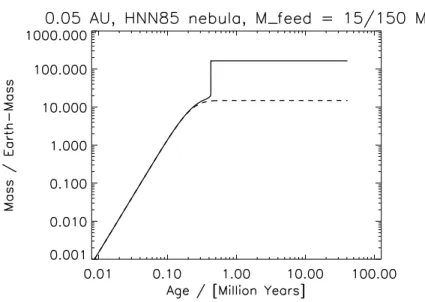
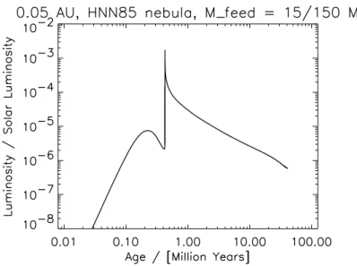
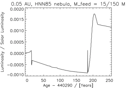
and Tscharnuter (2003) discuss how to set up and solve these equations and describe solutions relevant to the formation of stars and brown dwarfs. The authors calculate the collapse of cloud fragments with masses ranging from 0.05

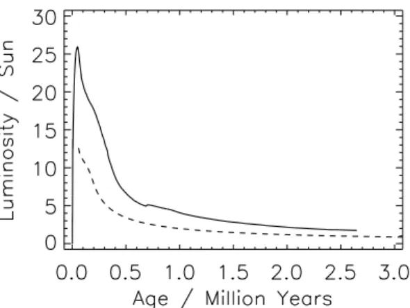
Figure 1: Early stellar evolution: collapse vs. Hayashi-line-contraction. Lu-minosity as function of age for a solar mass star. Full line: calculated from the protostellar collapse by Wuchterl and Tscharnuter (2003). Dashed line:

the quasi-hydrostatic contraction of an initially fully convective young star by D’Antona and Mazzitelli (1994).

to 10 M¯ and discuss the consequences for the hydrostatic stellar evolution on

the pre-main sequence.

7

Early stellar evolution — hydrostatic versus

collapse

We now look at the key differences between hydrostatic and collapse calcula-tions of early stellar evolution for the case of one solar mass. For the hydrostatic comparison case we follow Wuchterl and Tscharnuter (2003) and chose the cal-culations by D’Antona and Mazzitelli (1994), because atmospheric treatment, equations of state, opacities and convection treatment closely match those of Wuchterl and Tscharnuter (2003). Comparison to studies that include more physical processes (e.g., disc accretion or frequency dependent photospheric ra-diative transfer) can than be made by using existing intercomparisons of different hydrostatic studies to the D’Antona and Mazzitelli (1994) study. The luminos-ity as a function of age is shown for the collapse of a Bonnor-Ebert-sphere and a hydrostatic, contracting, initially fully convective young star in Fig. 1. Both studies use close to identical equations of state and calibrate mixing length the-ory of convection to the Sun. The two important differences are (1) the initial conditions and (2) the model equations.

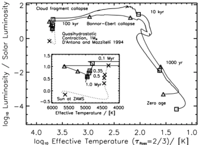
Bonnor-Figure 2: Protostellar collapse and early stellar evolution for a solar mass in a large theoretical Hertzsprung-Russel diagram. The collapse resulting from a fragmenting cloud (thick line) and a Bonner-Ebert-sphere (thin line) are compared to a quasi-hydrostatic pre-main sequence calculation (D’Antona and Mazzitelli (1994)). After Wuchterl and Klessen (2001).

Ebert-sphere as the initial gravitationally unstable cloud fragment. The calculation of pre-main sequence contraction starts with an initially high luminosity, fully convective structure.

Equations: Collapse is calculated using convective radiation fluid-dynamics with an equation of motion and time-dependent radiative and convective energy transfer. The calculation of pre-main sequence contraction as-sumes hydrostatic equilibrium and accounts for time-dependence only due to slow (very subsonic) gravitational contraction via the energy equation. To a good approximation the equations of the contraction-calculation, D’Antona and Mazzitelli (1994) are a hydrostatic limiting case of the col-lapse equations by used Wuchterl and Tscharnuter (2003).

The collapse calculation starts at zero luminosity (at the beginning of cloud collapse) and stays above the luminosity of the quasi-hydrostatic contraction calculation to beyond 2.5 Ma. The cloud collapse does not lead to a fully con-vective structure as assumed for the hydrostatic calculation. Even after most of the mass is hydrostatic, most of the Deuterium has been burnt and accretion effects have ceased to dominate, at approximately 0.7 Ma, the internal struc-ture stays partially radiative. The inner two thirds in radius remain radiative with a convective shell in the outer third of the radius — reminiscent of the present solar interior structure. Wuchterl and Tscharnuter (2003) found similar results from 2 down to 0.05 MSunBonnor-Ebert spheres, indicating that at least

consider-able mass range. The question then was whether the initial cloud conditions or the cloud environment or non-spherical effects could change the result. There-fore Wuchterl and Klessen (2001)10_{studied the fragmentation of a large, dense}

molecular cloud by isothermal hydrodynamics in three dimensions and followed the collapse of one of the resulting fragments, that was closest to a solar mass, throughout the non-isothermal phases to the end of accretion using the spher-ically symmetric equations of Wuchterl and Tscharnuter (2003). Despite the very different cloud environment — interactions with neighbouring fragments, competitive accretion, varying accretion rate, and orders of magnitude higher average accretion rates — the structure of the resulting, young solar mass star after one Ma was almost identical to the one resulting from the quiet Bonnor-Ebert collapse.

There were large differences during the embedded, high luminosity phases and the earliest pre-main sequence phase (cf. Fig. 2) but at 1 Ma, when the accretion-effects had become minor the over-all structure resulting from the Bonnor-Ebert-collapse was confirmed: a convective shell on top of a radiative interior. This has consequences for the observables of young stars at young ages. A solar precursor at 1 Ma should have twice the luminosity and an effective temperature that is 500 K higher than the one of the respective, fully convective structure resulting from a hydrostatic, high luminosity start.

The differences of the young Sun properties at 1 Ma properties are the result of a number of differences that result when early stellar evolution is calculated directly from the cloud collapse instead of the hydrostatic evolution of initially high luminosity, fully convective structures. The collapse calculation predict a series of changes to the classical picture. In summary (Wuchterl and Tscharnuter (2003)):

1. young solar mass stars are not fully convective when they have first settled into hydrostatic equilibrium,

2. their interior structure with an outer convective shell and an inner radia-tive core extending across 2/3 of the radius rather resembles the present Sun than a fully convective structure,

3. in the Hertzsprung-Russel-diagram they do not appear on the Hayashi line but to the left of it,

4. most of their Deuterium is burned during the accretion phases, 5. Deuterium burning starts and proceeds off-centre, in a shell,

6. therefore their is no thermostatic effect of Deuterium during pre-main sequence contraction and hence no physical basis for the concept of the stellar birthline, as proposed by Stahler (1988a).

7. These results are independent of the accretion rates during the cloud frag-mentation phase and non-spherical effects in the isothermal phase.

10_{The Wuchterl and Tscharnuter (2003) article was submitted in 1999 and subject to 4} years of peer reviewing by numerous reviewers.

These differences have important consequences for surface abundances (of Deu-terium and Lithium), rotational evolution, the stellar dynamo and stellar activ-ity that have to be worked out.

The observational tests are still to be done. What is needed are very young binary systems where masses can be determined independent of the model calcu-lationsand where the stellar parameters, effective temperature, surface gravity, or ideally the radius can be determined with sufficient accuracy. Furthermore the binary has to be sufficiently wide to exclude interactions during accretion and the evolution to the observed stage.

But for theoretical reasons alone — namely the requirement of a physical description of star formation and protostellar collapse — the dynamical models should be used when masses of stars, brown dwarfs and planets are determined from luminosities, effective temperatures, gravities or radii of those objects. At least for the ages that can be currently covered with such models, i.e. up to 10 Ma.

8

Protoplanetary Disks

In the previous sections we have shown how the problem of star formation can be solved when angular momentum ist neglected. The gravitational collapse of a cloud is then stopped when its central parts become opaque, heat up compres-sively and the thermal pressure finally re-balances gravity. Because pressure and gravity act isotropic the resulting structures, young stars, are spherical. When angular momentum is taken into account there is a second agent that can bring the collapse to a stop: inertia that gives rise to the centrifugal force. Even a slowly rotating cloud spins up dramatically as material collapses towards the centre reducing the axial distance by many orders of magnitude11 _under

con-servation of angular momentum. Unlike gas pressure, the centrifugal force is anisotropic and directed perpendicular to the axis of rotation. Hence collapse parallel to the axis of rotation is not modified by rotation. Gas can fall directly onto the central protostar along the polar axis and parallel to it towards the equatorial plane. The centrifugal force builds up during radial infall until it balances gravity at thecentrifugal radius,

Rcentrifugal=R 4_ω2

GM , (23)

for a cloud of mass, M, initial radius R, rotating with an initial angular fre-quencyω. Upon approach to that radius, the gas flow is more and more directed towards a collapse parallel to the axis of rotation. Finally material arrives in the equatorial plane. There, the vertical component of the central stars’ grav-itational force , i.e. the component parallel to the rotation axis, is zero. The radial component of the primary’s gravitational force is balanced by the cen-trifugal forces. The cloud has collapsed to a flattened structure in the stellar

11_{Typically by a factor of 1000 from 50 000 AU of the initial radius of a solar mass cloud} fragment to 50 AU for the disk radius.