Hammerstein systems parameters bounding through sparse polynomial
optimization
V. Cerone, D. Piga, D. Regruto
Abstract— A single-stage procedure to evaluate tight bounds on the parameters of Hammerstein systems from output measurements affected by bounded errors is presented. The identification problem is formulated in terms of polynomial optimization and relaxation techniques based on linear matrix inequalities are proposed to evaluate parameters bounds by means of convex optimization. The structured sparsity of the identification problem is exploited to reduce the computational complexity of the convex relaxed problem. Convergence proper-ties, complexity analysis and advantages of the proposed tech-nique with respect to previously published ones are discussed.
Index Terms— Bounded error identification, Hammerstein systems, Sparse LMI relaxation, Parameters bounds.
I. INTRODUCTION
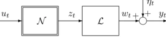
Identification of block-structured nonlinear systems, mod-eled by interconnected memoryless nonlinear gains and lin-ear dynamic subsystems, has attracted the attention of many authors in the last decades. Early works are summarized in the survey papers [1], [2] while an up-to-date collection of results and algorithms can be found in the recent book [3]. These models have been successfully used in many engi-neering fields, thanks to their ability to embed prior process structure knowledge like, e.g., the presence of nonlinearity either in the actuator or in the measurement equipment. The configuration we are dealing with in this note, commonly referred to as a Hammerstein model, is shown in Fig. 1; it consists of a static nonlinear part N followed by a linear dynamic system. The identification of such a model relies solely on input-output measurements, while the inner signal zt, i.e. the output of the nonlinear block, is not assumed to be available. A number of algorithm have been proposed in the literature to address such a problem. Among others we mention the over-parametrization method [4], [5], the subspace identification [6], the blind approach [7], the iterative method [8], the nonparametric approach [9] and the frequency domain method [10], [11]. In all the papers mentioned above, the authors assume that the measurement error ηt is statistically described. A worthwhile alternative to the stochastic description of measurement errors is the bounded-errors, or set-membership, characterization, where uncertainties are assumed to belong to a given set. The reader can find further details on this approach in the survey papers [12], [13] and in the book [14]. As far as set-membership identification of Hammerstein systems is concerned, Sznaier The authors are with the Dipartimento di Automatica e Informatica, Politecnico di Torino, corso Duca degli Abruzzi 24, 10129 Torino, Italy; e-mail: [email protected], [email protected], [email protected]; Tel: +39-011-564 7064; Fax: +39-011-564 7198
- N zt- L -?g
-ut wt yt
ηt + +
Fig. 1. Hammerstein system.
has recently shown in [15] that the problem is NP-hard in the size of the experimental data sequence pointing out the need of computationally tractable relaxations. In this paper we consider the identification of single-input single-output (SISO) Hammerstein models when the nonlinear block can be modeled by a linear combination of a finite and known number of nonlinear static functions, the linear dynamic part is described by an output error model and the output measurement errors are bounded. In a previous paper by the authors [16], a two-stage identification procedure is presented. First, parameters of the nonlinear block are tightly bounded using input-output data collected from the steady-state response of the system to a set of step inputs with different amplitudes. Then, through a dynamic experiment, for allutbelonging to a given input transient sequence{ut}, tight bounds on the inner signal are computed which, to-gether with noisy output measurements are used for bounding the parameters of the linear part. The main drawback of the procedure proposed in [16] is that it requires two different experiments where two specific input signals have to be used. On the contrary, when the input signal cannot be arbitrarily chosen, a one-step procedure without particular constraints on the input signal is required. In this paper an LMI-relaxation based one-stage algorithm is proposed to compute bounds on the parameters of both the nonlinear and the linear subsystems without constrains on the class of input signals. The paper is organized as follows. Background results on the relaxation of semialgebraic optimization problems through the theory of moments is presented in Section II. Section III is devoted to the problem formulation. In Section IV we show that computation of tight parameters bounds requires the solution to nonconvex optimization problems. The proposed LMI relaxation-based technique, together with a detailed analysis of its properties, is described in Section V. A simulated example is reported in Section VI.
II. NOTATION AND BACKGROUND RESULTS ON CONSTRAINED POLYNOMIAL OPTIMIZATION In this section we briefly review some preliminary results on the relaxation of sparse polynomial optimization problems
through a hierarchy of semidefinite programming (SDP) problems of increasing dimension. The reader is referred to [17] and the references therein for further details.
A. Polynomial representation and theory of moments
Let us denote with Pn
m[x] the space of real-valued poly-nomials of the degree at most m in the variable x = [x1, x2, . . . , xn]T ∈ Rn and let h be the canonical ba-sis of Pn m[x], i.e. h = [ 1x1x2 · · · xnx12x1x2 · · · x1xn x2 2x2x3 · · · xn2 · · · x31 · · ·xmn ]T
.Let us define the setAm as Am = {α∈Nn0 :
∑n
i αi≤m}, where αi is the i-th component of the vector α and Nn
0 denotes the set of
n-dimensional nonnegative integers vectors. Then, the basis h of the spacePmn[x]can be written ash={xα}α∈Am, where xα=xα1 1 x α2 2 · · ·x αn n .
Let f and gs be in Pmn[x]. We denote the sequence f =
{fα}α∈Am andgs={gsα}α∈Am as the coefficients of the polynomials f and gs, respectively, on the basis hm, i.e. f(x) = ∑ α∈Am fαxα,gs(x) = ∑ α∈Amgsαx α.
Letp={pα}α∈Ambe the sequence of moments (up to order m) of a probability measureµonRn, i.e. pα=
∫
xαµ(dx) andMm(p)be the truncated moment matrix associated with the distributionµ, i.e.Mm(p) =
∫
hhTµ(dx). Let us denote
with Mm(gkp) the localizing matrix associated with the sequence of momentspand with the polynomialgk(x). The reader is referred to [18] for details on the construction of the localizing matrix associated with a polynomial.
B. LMI-relaxation for polynomial optimization problems
The LMI-relaxation technique based on the theory of moments and proposed in [18] is briefly reviewed here. Let us consider the constrained optimization problem
f⋆= min
x∈Sf(x), (1)
wheref ∈ Pmn[x] andS ⊆Rn is a compact semialgebraic set defined as
S={x∈Rn:gs(x)≥0, s= 1, . . . ,Ξ}, (2) wheregsis a real-valued polynomial in the variablex∈Rn of degree ds = deg(gs), i.e. gs ∈ Pdns[x]. Let δ ∈ N be such that 2δ ≥ max{m,max
s ds} and h = {x α}
α∈A2δ be the canonical basis of the space P2nδ[x]. Indeed, f and gs belong toP2nδ[x].
Now, let us consider the SDP problem fδ = min p ∑ α∈An 2δ fαpα s.t. Mδ(p)≽0, Mδ−d˜s(gsp)≽0, s= 1, . . . ,Ξ(3) where d˜s = ⌈d s 2 ⌉
, p = {pα}α∈A2δ is the sequence of moments up to order2δof some probability measureµwith support onS, whileMδ(p)is the moment matrix associated with the momentspandMδ−ds˜(gsp)is the localizing matrix associated with the polynomialgs. Problem (3) is referred to as LMI-relaxed problem of orderδof the original polynomial problem (1). The solution fδ to the convex problem (3) is
a lower bound of the global optimumf⋆ of the nonconvex problem (1). Besides, under mild conditions, fδ converges tof⋆as the relaxation orderδgoes to infinity. Although the convergence properties are guaranteed as the relaxation order goes to infinity, exact global optimum f⋆ can obtained in practice with a reasonably low relaxation order (see [19] for a collection of problems solved with relaxation order less than 5). Unfortunately, due to high computational complexity, the discussed LMI-relaxation is restricted to polynomial prob-lems with a small number of variables, in general not greater than 10 for relaxation order smaller than 4. Several efforts on the reduction of LMI relaxation complexity, by exploiting the structured sparsity of the original polynomial problems, have been carried out in recent years (see, e.g., [20], [21], [22]). Roughly speaking, an optimization problem has a structured sparsity when the functional and each constraint defining the feasible region involve only a small subset of variables. In the next section we describe the relaxation technique presented in [23] in the spirit of the work of Waki et al [21]. Such a technique exploits the sparsity in the original polynomial problems to formulate a sparse version of the SDP-relaxation previously described, in order to extend the applicability of such a methodology to medium and large scale problems.
C. Sparse LMI-relaxation for polynomial problems
Let us consider the optimization problem (1) withS as in (2). LetI0 ={1, . . . , n} be the union of a collection of R
sets Ir ⊂ {1, . . . , n}, that is {1, . . . , n} = R
∪
r=1
Ir. Further, let us partition the index setS0={1, . . . ,Ξ}intoRdisjoint
setsSr,r= 1, . . . , R.
Let h(Ir) be the canonical basis of the polynomial
Pnr
m[x(Ir)], where x(Ir) = {xi|i∈ Ir}. Let us construct the partial moment matrixes Mm(p,Ir) (respectively the partial localizing matrixes Mm(gsp,Ir)) by retaining only those rows and columns of the moment matrix Mm(p) (respectively of the localizing matrix Mm(gsp)), where the variables pα are such that supp(α) ∈ Ir, with supp(α) denoting the support of the vectorα.
For a givenδ∈N such that 2δ≥max{m,max
s ds}, let us define the SDP problem
fspδ = min p ∑ α∈A2δ fαpα s.t. Mδ(p,Ir)≽0 (4) Mδ−ds˜(gsp,Ir)≽0, s∈ Sr, r= 1, . . . , R. Let us consider the following assumptions.
Assumption 1: For everyr= 1, . . . , Rand for every s∈
Sr, the constraintgs(x)≥0definingS in (2), depends only on the variablesx(Ir) ={xi|i∈ Ir}.
Assumption 2: The objective functionf can be written as f =
R
∑
r=1
fr, withfr∈ Pmn[x(Ir)], for everyr= 1, . . . , R.
Assumption 3: There exists a value G > 0 such that
Assumption 4: For everyr= 1, . . . , R−1, Ir+1∩ r ∪ j=1 Ij ⊆ Iq, for someq≤r. According to [23], the following result holds.
Theorem1: Under Assumptions 1 and 2 we have: fspδ ≤fspδ+1 ≤f∗. Furthermore, if also Assumptions 3 and 4 are satisfied, then lim
δ→∞f δ sp=f∗.
An implementation of the discussed sparse LMI-relaxation can be found in the Matlab package SparsePOP [24], which exploits the SDP solvers SeDuMi [25] and SDPA [26].
III. PROBLEM STATEMENT
Consider the SISO discrete-time Hammerstein model de-picted in Fig. 1. The nonlinear block maps the input signalut into the unmeasurable inner variableztthrough the following nonlinear function zt= nγ ∑ k=1 γkψk(ut), t= 1, . . . , N; (5) where (ψ1,...,ψnγ) is a known basis of nonlinear functions and N is the length of data sequence. The linear dynamic block L, supposed to be stable, is modeled by a discrete-time system transforming zt into the noise-free output wt according to equation wt=− na ∑ i=1 aiwt−i+ nb ∑ j=0 bjzt−j. (6) Letyt be the noise-corrupted output
yt=wt+ηt. (7)
Measurements uncertainty is known to range within given bounds∆ηt, i.e.,
|ηt|≤∆ηt. (8)
Unknown parameter vectors γ ∈ Rnγ and θ ∈ Rnθ are defined, respectively, as γ = [γ1 γ2 . . . γnγ
]T
and θ = [a1 . . . ana b0 b1 . . . bnb]T, with nθ = na +nb+ 1. It must be pointed out that the parametrization of the structure of Fig. 1 is not unique. As a matter of fact, any parameters set ˜bj = α−1bj, j = 0,1, . . . , nb, and γ˜k = αγk, k = 1,2, . . . , nγ, for some nonzero and finite constantα, provides the same input-output behaviour. Thus, any identification procedure cannot perceive the difference between parameters
{bj, γk}and{α−1bj, αγk}. To get a unique parametrization we assume, without loss of generality, that the steady-state gain of the linear part be one, i.e.
na ∑ i=1 ai= 1 + nn ∑ j=0 bj. (9)
In this paper we address the problem of deriving bounds on the parametersγ andθ consistently with given measure-ments, error bounds and the assumed model structure.
IV. EVALUATION OF TIGHT PARAMETERS UNCERTAINTY INTERVALS
The mapping between the input signalut and the noise-free outputwtfor the Hammerstein model in Fig. 1 can be obtained by substituting (5) in (6), which leads to the relation
wt=− na ∑ i=1 aiwt−i+ nb ∑ j=0 nγ ∑ k=1 bjγkψk(ut−j). (10) Therefore, from (7) and (10), we get the following mapping between the input signal and the output measurement:
yt=− na ∑ i=1 ai(yt−i−ηt−i) + nb ∑ j=0 nγ ∑ k=1 bjγkψk(ut−j) +ηt. (11) Indeed, the setDγθη of all the Hammerstein system param-eters (γ, θ) and the noise samples ηt consistent with the measurement data sequence, the assumed model structure and the error bounds is described by (8), (9) and (11), i.e.
Dγθη= { (γ, θ, η)∈Rnγ+nθ+N: yt=− na ∑ i=1 ai(yt−i−ηt−i)+ + nb ∑ j=0 nγ ∑ k=1 bjγkψk(ut−j) +ηt, |ηr| ≤∆ηr, na ∑ i=1 ai= 1 + nn ∑ j=0 bj, t=na+ 1, . . . , N; r= 1, . . . , N } , (12) which is rewritten as Dγθη= { (γ, θ, η)∈Rnγ+nθ+N: gt(γ, θ, η) =− na ∑ i=1 ai(yt−i−ηt−i)+ + nb ∑ j=0 nγ ∑ k=1 bjγkψk(ut−j) +ηt−yt≥0, gt+N(γ, θ, η) = na ∑ i=1 ai(yt−i−ηt−i)− − nb ∑ j=0 nγ ∑ k=1 bjγkψk(ut−j)−ηt+yt≥0, gr+2N(γ, θ, η) = ∆ηr−ηr≥0, gr+3N(γ, θ, η) = ∆ηr+ηr≥0, g4N+1(γ, θ, η) = na ∑ i=1 ai−1− nn ∑ j=0 bj≥0, g4N+2(γ, θ, η) =− na ∑ i=1 ai+ 1 + nn ∑ j=0 bj≥0, t=na+ 1, . . . , N; r= 1, . . . , N } . (13) withη = [η1, . . . , ηN] T
. Therefore, for every k= 1, . . . , nγ and j = 1, . . . , nθ, tight bounds on the parameters γk and θj can be computed by solving the optimization problems:
γ k=(γ,θ,ηmin)∈D γθη γk, γk= max (γ,θ,η)∈Dγθη γk, (14)
θj= min
(γ,θ,η)∈Dγθη
θj, θj= max
(γ,θ,η)∈Dγθη
θj. (15)
Thus, parameter uncertainty intervals on γk and θj are implicitly defined as P U Iγk =
[ γ k; γk ] and P U Iθj = [ θj; θj ]
. Note that the identification problems (14) and (15) are semialgebraic optimization problems. In fact, the objective function is linear and the feasible region
Dγθη is semialgebraic, since the constraints gt(γ, θ, η)≥0 and gt+N(γ, θ, η) ≥ 0 defining Dγθη in (13) are bilinear inequalities because of the product between the variable ai and the noise ηt−i as well as the product between the unknown parameters bj and γk. Because of bilinear constraints gt(γ, θ, η) ≥ 0 and gt+N(γ, θ, η) ≥ 0 defining the feasible region Dγθη, problems (14) and (15) are nonconvex. Therefore, standard nonlinear optimization tools (gradient method, Newton method, etc.) cannot be used since they can trap in local minima, which may prevent the computed uncertainty intervals from containing the true parameters, key requirement of any set-membership identification method. One possible solution to overcome such a problem is to relax identification problems (14) and (15) to convex optimization problems in order to numerically compute guaranteed parameter bounds.
V. EVALUATION OF PARAMETERS BOUNDS THROUGH CONVEX RELAXATION TECHNIQUES
Since (14) and (15) are semialgebraic optimization problems, they can be relaxed through a direct implementation of the dense LMI-relaxation technique described in Section II-B, which guarantees monotone converge to the exact parameters bounds defined in (14) and (15). In particular, for a given relaxation order δ, relaxing (14) and (15) through dense LMI-relaxation leads to SDP problems where the number of variables is O(N2δ) and the size of the largest LMI defining the feasible region is O(Nδ). Thus, the use of the dense LMI-relaxation technique is limited to Hammerstein system identification problems with a small number N of measurements (in general not greater than 5) because of an high computational burden. In order to handle a larger number of measurements, the particular structure of the identification problems (14) and (15) has been analyzed to apply the sparse LMI-relaxation presented in Section II-C. The following result shows that problems (14) and (15) have inherent structured sparsity.
Property1: Problems (14) (resp. (15)) enjoy the follow-ing features:
P1.1: The functional involves only the variableγk (resp. θj).
P1.2: For every t = na+ 1, . . . , N, the bilinear con-straintsgt≥0andgt+N ≥0depend only onnγ+nθ+na+1 variables, i.e. nγ nonlinear block parameters γ; nθ linear block parameters θ and na + 1 noise samples ηt−i, for i= 0,1, . . . , na.
P1.3: For every r = 1, . . . , N, constraints gr+2N ≥ 0 andgr+3N ≥0 depend only on the noise variable ηr.
P1.4: The linear constraints g4N+1≥0 andg4N+2≥0
depend only on the system parametersθ. A sparsity pattern in the identification problems (14) and (15) has been detected by exploiting results provided in Property 1. This allows us to formulate sparse SDP-relaxed problems for (14) and (15) as described in the following.
Let X ∈ Rnγ+nθ+N be the collection of the optimization variables for the identification problems (14) and (15), i.e. X = [γT θT ηT]T and let X
i the i-th component of the vector X. In such a way, the first nγ components of X are the nonlinear block parametersγ, the components from positionnγ + 1tonγ+nθ are the linear block parameters θ, while the components from position nγ +nθ + 1 to nγ + nθ +N are the noise variables η. Let us define the index sets Ir ⊂ {1,2, . . . , nγ+nθ+N} and Sr ⊂
{na+ 1, . . . , N, N+na+ 1, . . . ,2N+ 1, . . . ,4N+ 2} as Ir={1,2, . . . , nγ+nθ, nγ+nθ+r, nγ+nθ+r+ 1, . . . , nγ+nθ+r+na} forr= 1, . . . , N−na (16) S1={na+ 1, N+na+ 1, 2N+ 1,2N+ 2, . . . ,2N+na+ 1, 3N+ 1,3N+ 2, . . . ,3N+na+ 1,4N+ 1,4N+ 2} (17) Sr={na+r, N+na+r,2N+na+r,3N+na+r}, forr= 2, . . . , N−na (18) Note that the index sets Ir and Sr defined in (16)-(18) enjoy the following features.
Property2: For every r= 1, . . . , N−na, the index sets
Ir andSrare such that:
P2.1: The set of the variables indexes I0 = {1,2, . . . , nγ+nθ+N} is the union of the sets Ir, that isI0=
∪N−na r=1 Ir.
P2.2: The set of the constraints indexes S0 = {na+ 1, . . . , N, N+na+ 1, . . . ,2N,2N+ 1, . . .4N+ 2} defining Dγθη is the union of the sets Sr, that is
S0=
∪N−na r=1 Sr.
P2.3: The sets Srare mutually disjoint.
P2.4: For every s ∈ Sr, the polynomial polynomial constraint gs(γ, θ, η) ≥ 0 defining Dγθη depends only on the variablesX(Ir) ={Xi:i∈ Ir}.
P2.5: The functional of identification problems (14) and (15) depends only on the variablesX(Ir) ={Xi:i∈ Ir}.
P2.6: For everyr= 1, . . . , N−na−1, Ir+1∩ r ∪ j=1 Ij⊆ Ir.
Now, for a given relaxation orderδ≥1, let us consider the SDP problems γδ k = minp∈Dδ γθη ∑ α∈A2δ Γkαpα, γδk= max p∈Dδ γθη ∑ α∈A2δ Γkαpα (19) θδj = min p∈Dδ γθη ∑ α∈A2δ Θjαpα, θ δ j= max p∈Dδ γθη ∑ α∈A2δ Θjαpα (20) whereΓk ={Γkα}α∈A2δ (resp. Θj ={Θjα}α∈A2δ) is the coefficient vector of the function γk (resp. θj) in the basis h= {Xα}α∈A
2δ, which is the canonical basis of the real-valued polynomials of degree2δin the variables vector X. The feasible regionDδγθη is a convex set defined as
Dδ
γθη ={p:Mδ(p,Ir)≽0, r= 1, . . . , N−na
Mδ−1(gsp,Ir)≽0, s∈ Sr, r= 1, . . . , N−na} (21) whereMδ(p,Ir)is the moment matrix of orderδassociated to the variablesX(Ir) andMδ−1(gsp,Ir) is the localizing matrix (associated to the variables X(Ir)) taking into account the constraint gs ≥ 0 defining the original semialgebraic feasible regionDγθη.
Remark1: Since the linear block is known to be stable, stability constraints on the parameters a1, . . . , ana can be enforced in problems (14) and (15) with the method presented in [27] in order to improve the evaluation of the
parameter bounds evaluation.
The δ-relaxed uncertainty intervals, defined as P U Iδ γk = [ γδ k; γ δ k ] and P U Iδ θj = [ θδj; θδj ] , enjoy the following properties.
Property3: For everyk= 1, . . . , nγ and relaxation order δ≥1, the δ-relaxed uncertainty intervalP U Iδ
γk satisfy the following properties.
P3.1: Guaranteed relaxed uncertainty intervals. The intervalP U Iγδk is guaranteed to contain the true param-eter γk to be estimated, i.e.γk ∈ P U Iγkδ .
P3.2: Monotone convergence to tight uncertainty in-tervals. The interval P U Iγkδ becomes tighter as the relax-ation orderδincreases, that is P U Iδ+1
γk ⊆P U I δ
γk. Besides, P U Iγδk converges to the tight interval P U Iγk as the LMI relaxation order goes to infinity, that is:
lim δ→∞γ δ k=γk, δlim→∞γ δ k=γk. (22) The proof of Properties P3.1 and P3.2 (see [28] for details) follows from the properties of the index sets Ir and Sr highlighted in Property 2 and direct application of Theorem 1 to (14) and (15) and the corresponding SDP-relaxed problems (19) and (20). Similar results to Property 3 hold for the relaxed intervals P U Iδ
θj.
The computational complexity of the SDP problems (19) and (20) is now analyzed.
Property4: Computational complexity of the SDP-problems(19)and (20)
(i) The number of free optimization variablespis (N−na) ( nγ+nθ+na+ 1 + 2δ 2δ ) + −(N−na−1) ( nγ+nθ+na+ 2δ 2δ ) .
(ii) The feasible regionDδγθη is described by:
• N( −na moment matrixes, each one of size
nγ+nθ+na+ 1 +δ δ
)
,
• 2(N−na) + 2N+ 2localizing matrixes, each one of size ( nγ+nθ+na+δ δ−1 ) .
Technical details on the computation of number of optimization variables p and dimension of the LMIs describingDδ
γθη in (19) and (20) are reported in [28].
VI. ASIMULATED EXAMPLE
In this section we show the effectiveness of the presented parameter bounding procedure through a numerical example. The numerical computation is carried out on a 2.40-GHz Intel Pentium IV with 3 GB of RAM. The nonlinear block of the Hammerstein system considered here is modeled by the functionzt= 0.3ut+ 0.2u2t−ut3, i.e.γT= [γ1 γ2 γ3] =
[0.3 0.2 −1], while the linear part is a second order system with parameters θT = [a
1 a2 b1b2] = [1.8 0.9 1.6 2.1].
The input is a random sequence uniformly distributed be-tween [−1, +1]. Two different numerical experiments are performed. In the first one, only N = 50 number of mea-surements are expolited to compute the parameters bounds, while in the second experiment N = 250 data are used. The noise-free output wt is corrupted by random additive noise, uniformly distributed between[−∆ηt, +∆ηt]and the chosen error bounds ∆ηt are such that the signal to noise ratio SN Rw = 10 log { N ∑ t=1 w2t / N ∑ t=1 ηt2 } is equal to 27 db. Bounds on the parameters are evaluated by solving (19) and (20) for a relaxation orderδ= 2. Stability constraints on the linear block are enforced through the method described in [27]. Note that, in the considered example withN = 50, the number of optimization variable in (19) and (20) is 22,275, while the feasible region is defined by98 moment matrixes of size 55 and 396 localizing matrixes of size 10. On the other hand, if the sparsity was not taken into account, the number of variable of the SDP relaxed problems would be about 6 million and the feasible region would be described by a moment matrix of size5,886and396 localizing matrixes of size108, leading to an untractable optimization problem in the employed workstation. Results about the nonlinear and
Table I: Nonlinear block. Parameter central estimates (γc k), parameter bounds (γ
k,γk) and parameter uncertainties∆γk for N= 50andN = 250measurements.
N Parameter True γ k γ c k γk ∆γk Value 50 γ1 0.300 0.206 0.295 0.384 0.089 γ2 0.200 0.121 0.190 0.259 0.069 γ3 -1.000 -1.211 -1.000 -0.789 0.211 250 γ1 0.300 0.259 0.299 0.340 0.041 γ2 0.200 0.173 0.203 0.232 0.030 γ3 -1.000 -1.103 -1.000 -0.898 0.103 Table II: Linear block. Parameter central estimates (θcj), parameter bounds (θj,θj) and parameter uncertainties∆θj for N= 50andN = 250measurements.
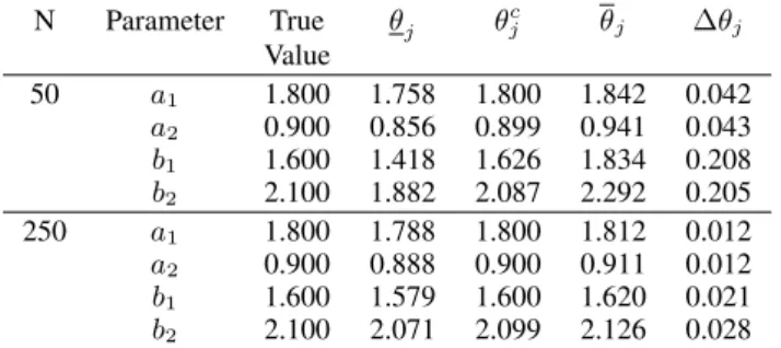
N Parameter True θj θc j θj ∆θj Value 50 a1 1.800 1.758 1.800 1.842 0.042 a2 0.900 0.856 0.899 0.941 0.043 b1 1.600 1.418 1.626 1.834 0.208 b2 2.100 1.882 2.087 2.292 0.205 250 a1 1.800 1.788 1.800 1.812 0.012 a2 0.900 0.888 0.900 0.911 0.012 b1 1.600 1.579 1.600 1.620 0.021 b2 2.100 2.071 2.099 2.126 0.028
the linear block are reported in Table I and II, respectively, which show the obtained parameter bounds, the central esti-matesγck andθjc as well as the parameter uncertainties∆γk and∆θj defined asγkc= γk+γ k 2 ,θ c j= θj+θj 2 ,∆γk = γk−γ k 2 and∆θj= θj−θj
2 . The CPU time taken by SeDuMi to solve
a single problem (19) and (20) is between 223 s and 263 s when the number of measurements N is equal to 50, and between 2442 s and 2578 s when N = 250. The reported results show that as the number of data increases (from N = 50toN = 250), the width of uncertainty intervals∆γk and∆θj decreases, as expected. Furthermore, we point out that the presented procedure provides satisfactory parameter uncertainty intervals, even for a small set of data (N = 50).
VII. CONCLUSIONS
A single-stage procedure to evaluate parameter uncertainty intervals for Hammerstein systems is proposed. The parame-ters bounds evaluation is formulated in terms of constrained polynomial optimization problems, whose approximate so-lutions can be computed by a hierarchy of SDP problems, which guarantees monotone convergence to global optima as the relaxation order increases. The particular structure of the original optimization problems made it possible a re-duction of the computational complexity of the SDP relaxed problems, preserving convergence to tight parameter bounds. The presented identification procedure can be also applied in the case of noise corrupted input sequence. As a matter of fact, in such a case, the identification problem can be still formulated in terms of sparse polynomial optimization problem by considering the noise samples on the input signal as variables.
REFERENCES
[1] S. Billings, “Identification of nonlinear systems — a survey,”IEE Proc. Part D, vol. 127, no. 6, pp. 272–285, 1980.
[2] R. Haber and H. Unbehauen, “Structure identification of nonlinear dynamic systems – a survey on input/uotput approaches,”Automatica, vol. 26, no. 4, pp. 651–677, 1990.
[3] E. Bai and F. Giri,Block-oriented nonlinear system identification, ser. Lecture notes in Control and Information sciences. Berlin: Springer. [4] F. Chang and R. Luus, “A noniterative method for identification using Hammerstein model,”IEEE Trans. Automatic Control, vol. AC-16, pp. 464–468, 1971.
[5] E. Bai, “An optimal two-stage identification algorithm for Hammerstein-Wiener nonlinear systems,” Automatica, vol. 34, no. 3, pp. 333–338, 1998.
[6] M. Verhaegen and D. Westwick, “Identifying MIMO Hammerstein systems in the context of subspace model identification methods,”Int. J. Control, vol. 63, no. 2, pp. 331–349, 1996.
[7] E. Bai and M. Fu, “A blind approach to Hammerstein model identifi-cation,”IEEE Trans. Signal Processing, vol. 50, no. 7, pp. 1610–1619, 2002.
[8] E. Bai and D. Li, “Convergence of the iterative Hammerstein system identification algorithm,” IEEE Trans. Automatic Control, vol. 49, no. 11, pp. 1929–1940, 2004.
[9] W. Greblicki and M. Pawlak, “Nonparametric identification of Ham-merstein systems,”IEEE Trans. Automatic Control, vol. 35, no. 2, pp. 409–418, 1989.
[10] E. Bai, “Frequency domain identification of Hammerstein models,” IEEE Trans. Automatic Control, vol. 48, no. 4, pp. 530–542, 2003. [11] A. Krzy˙zak, “On nonparametric estimation of nonlinear dynamic
systems by the Fourier series estimate,”Signal Processing, vol. 52, pp. 299–321, 1996.
[12] M. Milanese and A. Vicino, “Optimal estimation theory for dynamic sistems with set membership uncertainty: an overview,”Automatica, vol. 27(6), pp. 997–1009, 1991.
[13] E. Walter and H. Piet-Lahanier, “Estimation of parameter bounds from bounded-error data: a survey,” Mathematics and Computers in simulation, vol. 32, pp. 449–468, 1990.
[14] M. Milanese, J. Norton, H. Piet-Lahanier, and E. Walter, Eds., Bound-ing approaches to system identification. New York: Plenum Press, 1996.
[15] M. Sznaier, “Computational complexity analysis of set membership identification of Hammerstein and Wiener systems,” Automatica, vol. 45, no. 3, pp. 701–705, 2009.
[16] V. Cerone and D. Regruto, “Parameter bounds for discrete-time Ham-merstein models with bounded output errors,”IEEE Trans. Automatic Control, vol. 48, no. 10, pp. 1855–1860, 2003.
[17] M. Laurent, “Sums of squares, moment matrices and optimization over polynomials,”Emerging Applications of Algebraic Geometry, Vol. 149 of IMA Volumes in Mathematics and its Applications, M. Putinar and S. Sullivant (eds.), pp. 157–270, 2009.
[18] J. B. Lasserre, “Global optimization with polynomials and the problem of moments,”SIAM Journal on Optimization, vol. 11, pp. 796–817, 2001.
[19] D. Henrion and J. B. Lasserre, “Solving nonconvex optimization problems,”IEEE Control Systems Magazine, vol. 24, no. 3, pp. 72–83, 2004.
[20] M. Kojima, S. Kim, and H. Waki, “Sparsity in sums of squares of polynomials,”Mathematical Programming, vol. 103, pp. 45–62, 2005. [21] H. Waki, S. Kim, M. Kojima, and M. Muramatsu, “Sums of squares and semidefinite programming relaxations for polynomial optimization problems with structured sparsity,” SIAM Journal on Optimization, vol. 17, no. 1, pp. 218–242, 2006.
[22] P. Parrillo, “Exploiting algebraic structure in sum of squares pro-grams,”Positive Polynomials in Control, D. Henrion and A. Garulli (eds.), pp. 181–194, 2005.
[23] J. Lasserre, “Convergent semidefinite relaxations in polynomial opti-mization with sparsity,”SIAM Journal on Optimization, vol. 17, no. 1, pp. 822–843, 2006.
[24] H. Waki, S. Kim, M. Kojima, M. Muramatsu, and H. Sugimoto, “SparsePOP: a sparse semidefinite programming relaxation of poly-nomial optimization problems,” ACM Transaction on Mathematical Software, vol. 35, no. 2, 2008.
[25] J. F. Sturm, “Using SeDuMi 1.02, a MATLAB Toolbox for optimiza-tion over symmetric cones,”Optim. Methods Software, vol. 11, no. 12, pp. 625–653, 1999.
[26] K. Fujisawa, M. Fukuda, K. Kobayashi, M. Kojima, K. Nakata, M. Nakata, and M. Yamashita, “SDPA (semidefinite programming algorithm) users manual version 7.0.5,” Research Report B-448, Dept. of Mathematical and Computing Sciences, Tokyo Institute of Technology, 2008.
[27] V. Cerone, D. Piga, and D. Regruto, “Bounding the parameters of linear systems with stability constraints,” in Proc. of the American Control Conference 2010, 2010, pp. 2152–2157.
[28] ——, “Hammerstein systems identification through convex relaxation techniques,”Internal Report, vol. DAUIN, no. 2010/09/24, 2010.