Estimating likelihood of future crashes for crash-prone drivers

Original Research Paper

Estimating likelihood of future crashes for

crash-prone drivers

Subasish Das

, Xiaoduan Sun

, Fan Wang, Charles Leboeuf

a r t i c l e i n f o

Available online 31 March 2015

Keywords: Roadway safety Crash-prone drivers Crash risk Logistic regression Sensitivity

a b s t r a c t

At-fault crash-prone drivers are usually considered as the high risk group for possible future incidents or crashes. In Louisiana, 34% of crashes are repeatedly committed by the at-fault crash-prone drivers who represent only 5% of the total licensed drivers in the state. This research has conducted an exploratory data analysis based on the driver faultiness and proneness. The objective of this study is to develop a crash prediction model to esti-mate the likelihood of future crashes for the at-fault drivers. The logistic regression method is used by employing eight years'traffic crash data (2004e2011) in Louisiana. Crash predictors such as the driver's crash involvement, crash and road characteristics, human factors, collision type, and environmental factors are considered in the model. The at-fault and not-at-fault status of the crashes are used as the response variable. The developed model has identified a few important variables, and is used to correctly classify at-fault crashes up to 62.40% with a specificity of 77.25%. This model can identify as many as 62.40% of the crash incidence of at-fault drivers in the upcoming year. Traffic agencies can use the model for monitoring the performance of an at-fault crash-prone drivers and making roadway improvements meant to reduce crash proneness. From the findings, it is recommended that crash-prone drivers should be targeted for special safety programs regularly through education and regulations.

©2015 Periodical Offices of Chang'an University. Production and hosting by Elsevier B.V. on behalf of Owner. This is an open access article under the CC BY-NC-ND license (http:// creativecommons.org/licenses/by-nc-nd/4.0/).

1.

Introduction

Based on highway crash reports, conservatively speaking, more than 50% of crashes each year are caused by human errors. Engineers are always trying to make roadways more forgiving and vehicles more crashworthy, which has made considerable impact on highway safety, in order to account for

human error. Due to the persistent effort put forth by engi-neers, highway fatal crashes in the U.S. have finally reached the lowest number since 1960. Much of this effort has been spent on implementing crash countermeasures on highway facilities by enhancing the safety on roadway geometric fea-tures and traffic control devices. Safety education and enforcement, the other two elements in the 4E approach (emergency service is the fourth), also made strides in

*Corresponding authors. Tel.:þ1 225 288 9875.

E-mail addresses:subasishsn@gmail.com(S. Das),xsun@louisiana.edu(X. Sun). Peer review under responsibility of Periodical Offices of Chang'an University.

H O S T E D BY

Available online at

www.sciencedirect.com

ScienceDirect

journal homepage: www .e lsev ie r.com/locate/jtte

http://dx.doi.org/10.1016/j.jtte.2015.03.003

2095-7564/©2015 Periodical Offices of Chang'an University. Production and hosting by Elsevier B.V. on behalf of Owner. This is an open access article under the CC BY-NC-ND license (http://creativecommons.org/licenses/by-nc-nd/4.0/).

educating the general public on various safety risks and enforcing safety traffic laws.

In order to fulfill the hefty goal established by the American Association of State Highway and Transportation Officials (AASHTO) Highway Safety Strategy to cut traffic fatalities in half by 2020 and by Louisiana Strategic Highway Safety Plan for ‘Destination Zero Deaths’, it is important to have effective safety education and regulation programs while continually improving the highway infrastructure's safety. Since crash-prone drivers present a big adverse effect on highway safety, they should be effectively targeted in various safety education and enforcement programs. It is widely known that very young and very old drivers have the highest fatal crash rates, but this does not mean that these two groups commit the most crashes. People with similar personal traits could have very different levels of crash risk. Identifying high risk drivers and studying their characteristics are critical in order to further reduce the number of crashes through targeted safety education and enforcement programs.

Thus, a study was conducted at the University of Louisiana to study the impact of crash-prone drivers on safety and to predict how a driver's crash history could affect his/her crash occurrence(s) in the upcoming year. Logistic regression methods were used for the drivers with repeated crash in-volvements in previous years in order to establish relation-ships between driver responsibility and potential crash predictors. More importantly, the study was done to provide evidence for developing better and more efficient safety edu-cation programs and supporting targeted traffic laws or pro-grams based on these crash over-involved drivers.

This paper begins with the review of earlier studies that have attempted to relate various variables to develop models for crash-prone drivers. This review is followed by a descrip-tion of available data of nearly 2.08 million crash records for eight years'crash data. The next section provides discussion of model estimation results and its validation. In conclusion, an overall summary of findings on the model and their im-plications is given and some recommendations and direction for future research are provided.

2.

Literature review

Investigating crash-prone drivers' characteristics, exploring the relationship between drivers'past crash/citation history and their crash risk, and predicting drivers'future crash oc-currences from their previous crash history were the points focused on in many past studies.

The existence of crash-prone drivers was first recognized by Greenwood and Yule (1920). In their published paper, crash-prone drivers are defined as the drivers with a number of crashes higher than expected. In a study ofBlasco et al. (2003), crash-prone drivers are described as drivers with recurring crashes that are caused by human error, not by coincidence. A study conducted by Peck et al. (1971), concludes that it is quite difficult to accurately identify which driver will or will not cause crashes because of the statistical nature of crash frequencies. After analyzing five years'crash data (1993e1997) in Kentucky,Stamatiadis et al. (1999)found that about 2.1% of licensed drivers who were

charged with six or more points in the past 2 years accounted for nearly 5.3% of all crashes.

Predicting a driver's crash risk based on his/her past crash and traffic offence history is the topic of many investigations. The predictability of future crashes in terms of past violations or past crashes was investigated by Stewart and Campbell (1972). This study observed a four-year history of crash and violation records of North Carolina drivers to predict the future crashes. Through examining older drivers' previous conviction records and crash data, Daigneault et al. (2002) concluded that prior crashes would be a better predictor for crash risk than prior convictions. In a published study, Hauer et al. (1991)determined that the performance of their multivariate model for a crash would be improved by making right use of the driver's past crash records. A logistic regression model was developed by Chen et al. (1995) to identify crash-prone drivers based on their records prior to their at-fault crash involvements, which discovered that a model using prior at-fault crash data can recognize up to 23% more drivers who will have one or more at-fault crash involvements in the next 2 years than a model that uses the conviction information. After studying 17 logistic regression models, Gebers (1999) concluded that his models could correctly classify crash-involved drivers up to 27.6%. By deploying canonical correlation techniques in a subsequent research effort,Gebers and Peck (2003)achieved an accuracy level up to 27.2% from their best model to identify crash-prone driver. Chandraratna et al. (2006) studied Kentucky drivers to develop a crash prediction model that can be used to estimate the likelihood of a driver being at fault for a near future crash occurrence by using logistic regression technique. Although no model can be considered perfect, the modeling progress can be seen in research, especially in research from the Californian studies (Chen et al., 1995; Gebers, 1999). However, some researchers have voiced their skepticism over predicting crash-prone drivers (Gebers, 1999; Peck et al., 1971). In the recent years, research on at-fault drivers is becoming popular among researchers (Brar, 2014; Chandraratna and Stamatiadis, 2009; Currya et al., 2014; Goh et al., 2014; Greer et al., 2014; Harootunian et al., 2014; Karacasu and Er, 2011; Moghaddam and Ayati, 2014; Lee et al., 2014; Tseng, 2012; Yannis et al., 2005; Zhang et al., 2014). In contrast with the previously published works focusing on human factors for the risk analysis of crash-prone drivers, this research also takes into account roadway and crash var-iables in order to get a better insight on the risky drivers'crash proneness.

3.

Methodology

3.1. Dataset

The preliminary dataset was prepared from eight years (2004e2011) of crash data from Louisiana. It was arranged by merging three different tables (crash table, roadway table, and vehicle table) from the microsoft access dataset. For an indi-vidual crash record, a total of 371 crash attributes (possible explanatory variables) were collected. A total number of 2,076,009 crash records remained after deleting the records

that did not contain driver's license information. Out of 2.07 million crash records, 1,070,891 crash records were for at-fault drivers and the remaining 1,005,118 records contained records of not-at-fault drivers. Based on the proneness, 1,371,528 re-cords contained the information of non-crash-prone drivers, the rest 704,481 records the for crash-prone drivers. This big database was analyzed by using a graphical R package ‘ggplot2’(R Development Core Team, 2013; Wickham, 2009).

For the interest of the study, four types of drivers are defined. At-fault drivers are responsible for crash occurrence. Not-at-fault drivers are involved in a crash but not responsible for. Crash-prone drivers are involved with multiple crashes. Non-prone drivers are associated only one crash involvement. The drivers are grouped in four general categories for analysis purpose: at-fault prone drivers, at-fault prone drivers, not-at-fault non-prone drivers, and not-at-fault non-prone drivers.

In general about 4% of licensed drivers in Louisiana are involved in at least one crash each year. The number of drivers having crashes is summarized inTables 1 and 2. The infor-mation in the tables reveals that some drivers have crashes repeatedly within one year. The annual maximum number of crashes to a single at-fault driver is nine. Drivers causing multiple crashes annually accounted for about 10% of crashes occurred.

As expected, drivers holding a Louisiana driver's license cause the majority of crashes. About 66% and 34% of crashes are blamed on drivers with single crashes and with multiple crashes in eight years, respectively. These 34% of crashes are repeatedly committed by the crash-prone drivers only repre-senting 5% of licensed drivers in the state. In Fig. 1, the percentages of fatal crashes by both at-fault and not-at-fault drivers are shown. In the most recent analyzed year (2011), the percentage of fatal crashes for both categories of drivers increased sharply after a decline in the previous year.

Traffic crash databases contain many variables some of which are redundant in nature. The variable selection method

uses the related previous research findings with engineering judgment. The final variables selected for modeling are grouped as:

1. Human factor related variables (driver age, alcohol involvement, drug involvement, driver distraction, driver gender, and driver severity).

2. Crash related variables (crash hour, day of the week, collision type, and total severity).

3. Roadway related variables (alignment, lighting condition, and road type).

4. Environment related variables (weather). 5. Vehicle related variables (vehicle condition).

Developing models with too many variables does not serve the purpose in understanding the possible relationship be-tween the variables. A regression subset selection with an exhaustive search method is first performed to reduce the number of variables through linear regression. This task was performed by using R package ‘leaps’ (Lumley and Miller, 2013). The process is done by an exhaustive search for the best subsets of the variables in x for predictingy in linear regression, using an efficient branch-and-bound optimization algorithm. The adjustedR2value (variables that have black boxes at the highesty-axis value) of each of the categories would help to see the redundant categories. By adjusting theR2_{value, the best model doesn't include crash} hour, day of the week, road type, weather, total severity and vehicle condition. The number of variables in the final dataset reduces to ten for model development (Table 3). 3.2. At-fault and not-at-fault drivers

Both at-fault and not-at-fault drivers are divided into two other groups: crash-prone and non-crash-prone drivers. The graphical representation of the human factors in crashes is Table 1eNumbers of at-fault drivers with crashes.

No. of crash(es) in particular year 2004 2005 2006 2007 2008 2009 2010 2011 1 129,009 123,901 123,290 121,854 121,166 121,904 114,025 121,343 2 6076 5507 5801 5830 5346 5356 4818 2982 3 450 384 437 433 423 376 316 73 4 49 40 63 79 44 42 35 24 5 7 10 10 12 6 8 15 1 6 1 3 1 0 0 4 1 0 7 2 0 0 1 1 0 1 0 8 1 14 9 1 0 5 8 2 9 0 2 1 0 0 0 0 0

Table 2eNumbers of not-at-fault drivers with crashes. No. of crash(es) in particular year 2004 2005 2006 2007 2008 2009 2010 2011 1 123,050 119,375 120,373 118,439 117,085 115,298 109,672 114,799 2 4420 4399 4265 4110 3972 3717 3617 2520 3 197 190 197 167 164 160 144 66 4 17 25 14 32 18 9 23 24 5 1 2 2 5 5 2 4 1 6 0 1 6 0 0 0 1 0

displayed inFig. 2. InFig. 2(a), it's seen that the percentages of at-fault prone male drivers are higher than those of the other three groups. This clearly indicates a particular gender group's involvement in repeated at-fault crashes.Fig. 2(b)reveals that the percentages of at-fault prone younger drivers (15e24) involved in crashes are higher than the other three groups. On the other hand, the percentages of crashes from non-prone older drivers (55 plus) are higher than the other two groups. This clearly indicates a particular age group's involvement in repeated at-fault crashes over the years.

The distribution of crashes inFig. 2(c)presents that alcohol intoxicated at-fault drivers are involved in at least 5% of the total crashes while not-at-fault drivers are involved in 3% of the total crashes. Moreover, at-fault prone drivers are higher in percentage than not-at-fault prone drivers. The percentages of drug impaired and not-impaired drivers are shown inFig. 2(d). Over 3% of total drivers are drug impaired in at-fault drivers' crash record. Like the alcohol impaired statistics, drug impaired at-fault prone drivers are higher in percentage than not-at-fault prone drivers.

The percentages of distraction categories of the drivers are exhibited inFig. 2(e). Nearly 94% of not-at-fault drives are not distracted while driving. This percentage is lowered down to 65% for at-fault drivers. The remaining 35% of the drivers are distracted while driving. This clearly distinguishes the driving behavior of at-fault and not-at-fault drivers.Fig. 2(f) shows the percentage of driver severity for each of the four groups. From the data, it is found that at-fault drivers are involved in 0.7% of total driver fatalities while not-at-fault drivers are involved in 0.15% of total fatalities.

Fig. 2 unveils that at-fault prone drivers are higher in percentage in alcohol and drug intoxication, distraction, and driver fatalities than not-at-fault prone drivers. A particular group (male younger drivers) is also seen to be higher in percentage in at-fault prone drivers.

Fig. 3 represents two important roadway factors and patterns of collision types in four groups of drivers. In Fig. 3(a), it's found that curve-level related crashes are slightly higher in percentage in not-fault drivers than at-fault drivers. When the curve level is elevated, at-at-fault drivers are larger in percentage than not-at-fault groups. Fig. 1ePercentages of fatal crashes by crash-prone drivers.

Table 3eVariables and categories.

Category Frequency Percentage(%)

Faultiness At-fault 252,641 55.84 Not-at-fault 199,789 44.16 Alcohol No 432,800 95.66 Yes 19,630 4.34 Alignment Straight-level 390,153 86.23 Curve-level 28,946 6.40 Straight-level-elevated 12,419 2.74 On grade-straight 8960 1.98 On grade-curve 3500 0.77 Curve-level-elevated 3145 0.70 Hillcrest-straight 3441 0.76 Hillcrest-curve 519 0.11 Dip, hump-straight 479 0.11 Dip, hump-curve 118 0.03 Other 587 0.13 Unknown 163 0.04 Lighting Daylight 338,943 74.92

Dark-continuous street light 55,645 12.30 Dark-no street light 35,694 7.89 Dark-street light at intersection only 10,454 2.31 Dusk 7115 1.57 Dawn 3939 0.87 Other 340 0.08 Unknown 300 0.07 Driver severity No injury 367,608 81.25 Complaint 67,126 14.84 Moderate 15,199 3.36 Severe 1725 0.38 Fatal 772 0.17 Collision type Rear end 185,154 40.92 Right angle 68,717 15.19 Sideswipe-same direction 48,880 10.80 Single vehicle 49,381 10.91 Left turn-opposite direction 17,466 3.86 Left turn-angle 10,614 2.35 Left turn-same direction 8646 1.91

Head-on 6448 1.43

Right turn-opposite direction 2332 0.52 Right turn-same direction 6834 1.51 Sideswipe-opposite direction 9332 2.06 Other 38,626 8.54 Gender Male 258,096 57.05 Female 194,334 42.95 Driver age 15e24 137,462 30.38 25e34 109,029 24.10 35e44 77,223 17.07 45e54 63,907 14.13 55e64 37,620 8.32 65e74 17,154 3.79 75 plus 10,035 2.22 Driver distraction Not distracted 352,781 77.97 Unknown 68,022 15.03 Other inside 14,053 3.11 Other outside 11,606 2.57 Cell phone 4931 1.09

This clearly indicates that crash at-fault prone drivers have some difficulties in driving when the curve-level is elevated. Fig. 3(b)presents the driver's interaction with the roadway lighting condition. Not-at-fault drivers are involved in more crashes (percentage wise) in daylight than at-fault drivers. A specific condition like dark with continuous lightings displays an almost similar percentage of crashes for all four groups. On the other hand, no street lighting at night is a poor roadway condition. In this roadway condition, at-fault drivers are more vulnerable to crashes than not-at-fault drivers. As the database contains eight years of crash data,

this particular information can't be considered as a random incident. This information also emphasizes the importance of considering roadway and geometric variables in the modeling of at-fault crashes for crash-prone drivers. Collision type is also an important measure in crash-prone drivers'crash investigation. Not-at-fault drivers are involved in more rear-end crashes than at-fault drivers. Single vehicle run-off crashes are higher in percentage in at-fault drivers' group (Fig. 3(c)). At-fault drivers are involved in run-off crashes more than ten times of not-at-fault drivers.

4.

Model development

In this study, a logistic regression model is developed by using the dataset of crash-prone drivers. It is very important to note that there are different factors associated for a driver to be involved in crashes. Drivers involved in multiple crashes for a time span need to be studied in order to understand the driver's physical condition and interaction in the driving task. Table 3e(continued)

Category Frequency Percentage(%)

Other electronics inside 986 0.22

Others 51 0.01

Drugs

No 445,573 98.48

Yes 6857 1.52

Fig. 2eGraphics of human factors for four different driver groups based on (a) driver gender, (b) driver age, (c) alcohol involvement, (d) drugs involvement, (e) driver distraction, and (f) driver severity.

The general driving population can be considered as not-at-fault drivers. There is some argument that defensive drivers are mostly not-at-fault drivers. For their defensive driving techniques, they are not exposed to crash causation. So, it's important to find out the different set of crash and driver characteristics with this group of drivers. Logistic regression has good potential to analyze this sort of dataset. The reason is that logistic regression is a form of regression, which is used when the response variable is binary. Logistic regression techniques are particularly beneficial when the effects of more than one explanatory variable are important. In this analysis, the response variable is the fault status of the driver. The probability of occurrence of an at-fault crash for theith_{case is:}

pi¼_1þ1_eli (1)

li¼a0þb1Y1iþb2Y2iþ/þbjYjiþ/þbnYni (2) whereliis the linear combination of predictor variable cate-gories; bj is coefficient estimated using the maximum

likelihood method;Yjiis the explanatory predictor variable as listed inTable 4.

For the logistic model, Eq.(1)can be rewritten as commonly rearranged as the following:

lg pi 1pi ¼a0þb1Y1iþb2Y2iþ/þbjYjiþ/þbnYni (3) Here, probability of not-at-fault crashes by crash-prone drivers is equal to 1 minus probability of at-fault crashes by crash-prone drivers.

The logistic model in R software is a special case of the generalized linear model (GLM), implemented in R by the ‘glm’ method (R Development Core Team, 2013). Here the response variable (at-fault or not-at-fault crashes) is changed as a function of predictor variables. The output of the developed logistic model is listed in Table 5. The null deviance measures the variability of the dataset, compared to the residual deviance, which measures the variability of the residuals, after fitting the model. These deviances can be used like the total and residual sum of squares in a linear Fig. 2e(continued).

model to estimate how well it fits; the fit value of the model is 0.18. So, less than 19% of the deviance in the model has been explained by the explanatory categories.

Table 5shows the results of the model. The odds ratio is a measure of effect size, describing the strength of association or non-independence between two binary data values, here at-fault and not-at-fault crashes. The odds ratio of ‘Alcohol Yes’is 1.29 which implies that crash-prone drivers with at-fault crashes have a 29% higher chance of being involved in at-fault crashes than not-at-fault crashes in the upcoming year. The odds ratios having values greater than 1 are the contributing factors for at-fault crashes in the future. The ANOVA table is listed in Table 5. The table demonstrates higher significance for all nine variables. The significance of the variables is shown in the last column ofTable 4.

To compare linear models we often use the adjustedR2_{. A} more general measure for these, which is also applicable to generalized linear models, is the Akaike information criterion (AIC). This adjusts the residual deviance for the number of predictors. The AIC for the model is 508,379. The model has the null deviance of 621,013 on 452,429 degrees of freedom.

The residual deviance of the model is 508,281 on 452,381 de-grees of freedom.

The model is tested by removing one or several categories. Each time the comparison of the model is tested with the newer one. One simple indicator of the model's performance is AIC value. This model shows the lower AIC value than the others which clearly indicates that removal of one or several categories alters the model.

The success of this logistic regression model can be assessed with the receiver operating characteristic (ROC) curve. The ROC curve is a plot of the sensitivity (proportion of true positives) of the model prediction against the comple-ment of its specificity (proportion of false positives), at a series of thresholds for a positive outcome. The logistic model gives the probability that each location has changed; this can be changed to a binary outcome (at-fault vs. not-at-fault) by selecting a threshold.

The sensitivity and specificity can be computed at any threshold by comparing the predicted with the actual change. The sensitivity is defined as the ability of the model to find the ‘positive’criteria that actually changes the response variable: Fig. 2e(continued).

S1¼P=T1 (4) whereS1is sensitivity, Pis number of true positives, T1 is number of total positives.

The other side to a model's performance, the specificity, can be defined as the proportion of ‘negatives’ that are correctly predicted:

S2¼N=T2 (5)

whereS2is specificity, Nis number of true negatives,T2is number of total negatives.

Fig. 4exposes that the developed model is quite successful in identifying the probability of at-fault and not-at-fault crashes for the crash-prone drivers. The horizontal ticks of Fig. 4represent errors: either false positives or false negatives.

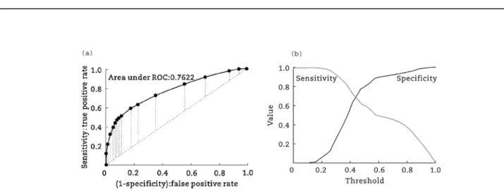
A graph of the sensitivity (on they-axis) vs. the false pos-itive rate (on thex-axis) at different thresholds is known as receiver operating characteristic (ROC) curve. In fact, even at the lower thresholds, the model predicts most of the true positives with few false positives, so the curve would rise rapidly from (0, 0). The closer the curve comes to the left-hand border and then the top border of the graph (ROC space), the more accurate the model is which means that it has high sensitivity and specificity even at low thresholds. The closer the curve comes to the diagonal, the less accurate the model is. This is because the diagonal represents the random case: the model predicts at random, so the chance of a true positive is equal to that of a false positive, at any threshold.

The ROC curve can be summarized by the area under the curve (AUC). The observed area under the ROC curve (AUC) is Fig. 2e(continued).

0.7622 for the model, illustrated inFig. 5(a), which would be generally accepted as a fair value in a 0.5e1 scale. The sensitivity-specificity curve is displayed inFig. 5(b).

5.

Conclusions

The main objective of this study is to use logistic regression technique and develop crash prediction models for the at-fault crashes of crash-prone drivers in upcoming years. The eight years crash data analysis introduced in this paper has demonstrated that crash-prone drivers need to be carefully targeted in safety education and traffic law enforcement

programs because their over-involvement in crashes presents a large adverse effect on roadway safety.

At first, the database is analyzed by means of basic descriptive statistical methods generating a number of inter-esting facts. Younger male drivers (15e34) are more vulner-able to crash proneness. Crash-prone drivers have issues with roadways with no illumination. Fatality and severity rates are higher in at-fault crash-prone drivers. Alcohol and drug impaired driving are seen more frequently in crash-prone drivers than in non-prone ones. Single vehicle run-off crashes are higher in percentage in the at-fault drivers'group. At-fault prone drivers are involved in more curved-aligned roadways than the other drivers. Secondly, the logistic regression Fig. 3eGraphics of roadway and crash factors for four different driver groups based on (a) roadway alignment, (b) roadway lighting condition, and (c) collision type.

method is used by employing eight years of crash data (2004e2011) for Louisiana. Crash predictors like the driver's crash involvement, crash and road characteristics, human factors, crash type, and environmental factors are used in this study. The at-fault and not-at-fault status of the crashes are used as the dependable variable. The developed model can be used to correctly classify at-fault crashes up to 62.40% with specificity of 77.25%. This model can identify as many as

62.40% of the crash incidence of at-fault drivers in the up-coming year. Traffic agencies can use the model for moni-toring the performance of an at-fault prone driver as well as make improvements to the roadways to reduce crash proneness.

It is determined that crash-prone drivers should be tar-geted by special safety programs regularly through education and regulations. For instance, a state motor vehicle Fig. 3e(continued).

Table 4eResults of logistic regression model.

Predictor variable Estimate Std. error zvalue Pr(>jzj) Odds ratio 2.5% 97.5% (Intercept) 2.7787 0.0794 35.0010 <2e-16 16.0983 13.8107 18.8552 Drugs Yes 0.7130 0.0330 21.6220 <2e-16 2.0402 1.9128 2.1768 Alcohol Yes 0.2565 0.0196 13.0860 <2e-16 1.2924 1.2438 1.3431 Alignment Curve-Level-Elevated 0.1611 0.0472 3.4140 0.000641 0.8512 0.7761 0.9338 Alignment Dip, Hump-Curve 0.1332 0.2343 0.5690 0.569547 0.8753 0.5552 1.3936 Alignment Dip, Hump-Straight 0.0919 0.1079 0.8520 0.39437 0.9122 0.7386 1.1277 Alignment Hillcrest-Curve 0.2090 0.1120 1.8660 0.062038 0.8114 0.6520 1.0115 Alignment Hillcrest-Straight 0.3372 0.0420 8.0260 1e-15 0.7138 0.6574 0.7750 Alignment On Grade-Curve 0.1140 0.0486 2.3480 0.018891 1.1208 1.0193 1.2331 Alignment On Grade-Straight 0.3150 0.0288 10.9420 <2e-16 0.7298 0.6898 0.7722 Alignment Other 0.4529 0.0985 4.5960 0.0000043 0.6358 0.5241 0.7713 Alignment Straight-Level 0.2530 0.0158 15.9850 <2e-16 0.7765 0.7528 0.8009 Alignment Straight-Level-Elevated 0.3395 0.0256 13.2830 <2e-16 0.7121 0.6773 0.7487 Alignment Unknown 1.0472 0.1882 5.5650 2.62e-08 0.3509 0.2428 0.5080 Lighting Dark-No Street Lights 0.3703 0.0175 21.1230 <2e-16 1.4481 1.3992 1.4987 Lighting Dark-Street Light At Intersection 0.1128 0.0251 4.4920 0.00000705 1.1195 1.0657 1.1760 Lighting Dawn 0.1620 0.0388 4.1780 0.0000294 1.1758 1.0898 1.2687 Lighting Daylight 0.1214 0.0106 11.4800 <2e-16 1.1291 1.1059 1.1527 Lighting Dusk 0.0779 0.0287 2.7190 0.006547 1.0811 1.0220 1.1435 Lighting Other 0.2466 0.1270 1.9410 0.052262 1.2796 0.9982 1.6431 Lighting Unknown 0.1786 0.1446 1.2350 2.17e-01 0.8365 0.6305 1.1119 Collision_Type Left Turn-Angle 0.1975 0.0351 5.6220 1.89e-08 0.8207 0.7661 0.8792 Collision_Type Left Turn-Opposite Direction 0.2366 0.0326 7.2580 3.93e-13 0.7893 0.7405 0.8414 Collision_Type Left Turn-Same Direction 0.2490 0.0366 6.8060 1.00e-11 0.7796 0.7256 0.8375 Collision_Type Other 0.1564 0.0304 5.1510 2.59e-07 1.1693 1.1017 1.2410 Collision_Type Rear End 0.2020 0.0287 7.0410 1.9e-12 0.8171 0.7724 0.8644 Collision_Type Right Angle 0.1633 0.0294 5.5620 2.67e-08 0.8493 0.8018 0.8996 Collision_Type Right Turn-Opposite Direction 0.1454 0.0531 2.7390 0.006154 0.8647 0.7792 0.9595 Collision_Type Right Turn-Same Direction 0.3006 0.0385 7.8140 5.54e-15 0.7404 0.6866 0.7983 Collision_TypeSideswipe-Opposite Direction 0.2485 0.0361 6.8760 6.16e-12 0.7800 0.7266 0.8372 Collision_Type Sideswipe-Same Direction 0.3267 0.0299 10.9170 <2e-16 0.7213 0.6802 0.7649 Collision_Type Single Vehicle 2.1865 0.0329 66.3920 <2e-16 8.9040 8.3476 9.4979 Driver_Gender Male 0.3672 0.0069 53.3560 <2e-16 1.4436 1.4243 1.4633 Driver_Severity Fatal 0.5627 0.1287 4.3710 1.24e-05 1.7554 1.3709 2.2719 Driver_Severity Moderate 0.3912 0.0223 17.5140 <2e-16 1.4788 1.4155 1.5450 Driver_Severity No Injury 0.6080 0.0101 60.0860 <2e-16 1.8368 1.8007 1.8736 Driver_Severity Severe 0.5201 0.0646 8.0510 8.19e-16 1.6822 1.4827 1.9101 Driver_Age25e34 0.5109 0.0093 54.7770 <2e-16 0.5999 0.5891 0.6110 Driver_Age35e44 0.7060 0.0103 68.4500 <2e-16 0.4936 0.4837 0.5037 Driver_Age45e54 0.7144 0.0109 65.3360 <2e-16 0.4895 0.4791 0.5001 Driver_Age55e64 0.6505 0.0131 49.7300 <2e-16 0.5218 0.5086 0.5353 Driver_Age65e74 0.3437 0.0179 19.1850 <2e-16 0.7091 0.6847 0.7345 Driver_Age75 plus 0.4256 0.0243 17.4980 <2e-16 1.5305 1.4594 1.6053 Driver_Distraction Not Distracted 3.1110 0.0721 43.1610 <2e-16 0.0446 0.0386 0.0512 Driver_Distraction Other Electronics Inside 0.7837 0.1374 5.7030 1.18e-08 0.4567 0.3502 0.6005 Driver_Distraction Other Inside 0.8995 0.0938 9.5860 <2e-16 2.4583 2.0434 2.9526 Driver_Distraction Other Outside 0.5703 0.0798 7.1440 9.04e-13 0.5654 0.4824 0.6597 Driver_Distraction Others 0.6509 0.5394 1.2070 0.227548 0.5216 0.2027 1.7753 Driver_Distraction Unknown 1.3430 0.0728 18.4550 <2e-16 0.2611 0.2257 0.3003

Table 5eANOVA table.

Df Deviance Resid.df Resid.dev Pr(>Chi)

Null 452,429 621,013

Drugs 1 1310 452,428 619,703 <2e-16

Alcohol 1 1592 452,427 618,111 <2e-16

Alignment 11 3520 452,416 614,591 <2e-16

Lighting 7 4005 452,409 610,587 <2e-16

Collision type 11 28,361 452,398 582,225 <2e-16

Driver gender 1 3416 452,397 578,809 <2e-16

Driver severity 4 4472 452,393 574,337 <2e-16

Driver age 6 10,871 452,387 563,466 <2e-16

registration office can work with enforcement agencies to establish a driver's license reviewing program that has the authority to send warnings or to suspend a driver's license, or to request that the driver take a mandatory safety course if the driver has multiple crashes within a short time period.

r e f e r e n c e s

Blasco, R.D., Prieto, J.M., Cornejo, J.M., 2003. Accident probability after accident occurrence. Safety Science 4 (6), 481e501. Brar, S.S., 2014. Estimating the over-involvement of suspended,

revoked, and unlicensed drivers as at-fault drivers in California fatal crashes. Journal of Safety Research 50, 53e58. Chandraratna, S., Stamatiadis, N., 2009. Quasi-induced exposure method: evaluation of not-at-fault assumption. Accident Analysis and Prevention 41 (2), 308e313.

Chandraratna, S., Stamatiadis, N., Stromberg, A., 2006. Crash involvement of drivers with multiple crashes. Accident Analysis and Prevention 38 (3), 532e541.

Chen, W., Cooper, P., Pinili, M., 1995. Driver accident risk in relation to the penalty point system in British Columbia. Journal of Safety Research 26 (1), 9e18.

Currya, A.E., Pfeiffer, M.R., Myers, R.K., et al., 2014. Statistical implications of using moving violations to determine crash responsibility in young driver crashes. Accident Analysis and Prevention 65, 28e35.

Daigneault, G., Joly, P., Frigon, J.Y., 2002. Previous convictions or accidents and the risk of subsequent accidents of older drivers. Accident Analysis and Prevention 34 (2), 257e261. Gebers, M.A., 1999. Strategies for Estimating Driver Accident Risk

in Relation to California's Negligent-operator Point System. California Department of Motor Vehicles, Sacramento. Gebers, M.A., Peck, R.C., 2003. Using traffic conviction correlates

to identify high accident-risk drivers. Accident Analysis and Prevention 35 (6), 903e912.

Goh, K., Currie, G., Sarvi, M., et al., 2014. Factors affecting the probability of bus drivers being at-fault in bus-involved accidents. Accident Analysis and Prevention 66, 20e26. Greenwood, M., Yule, G.U., 1920. An inquiry into the nature of

frequency distributions representative of multiple happenings with particular reference to the occurrence of multiple attacks of disease or of repeated accidents. Journal of Royal Statistical Society 83 (2), 255e279.

Greer, A.M., Macdonald, S., Mann, R.E., 2014. Stress, adrenaline, and fatigue contributing to at-fault collision risk: quantitative and qualitative measures of driving after gambling. Journal of Transport and Health. http://dx.doi.org/10.1016/j.jth.2014.11.001. Harootunian, K., Lee, B.H.Y., Aultman-Hall, L., 2014. Odds of fault and factors for out-of-state drivers in crashes in four states of the USA. Accident Analysis and Prevention 72, 32e43. Hauer, E., Persaud, B.N., Smiley, A., et al., 1991. Estimating the

accident potential of an Ontario driver. Accident Analysis and Prevention 23 (2/3), 133e152.

Karacasu, M., Er, A., 2011. An analysis on distribution of traffic faults in accidents, based on driver's age and gender: Fig. 4eSuccesses of models. (a) Success of the logistic model. (b) Success of the model (sensitivity: 0.624, specificity: 0.7725).

Eskisehir case. Procedia-Social and Behavioral Sciences 20, 776e785.

Lee, J., Abdel-Aty, M., Choi, K., 2014. Analysis of residence characteristics of at-fault drivers in traffic crashes. Safety Science 68, 6e13.

Lumley, T., Miller, A., 2013. Leaps: Regression Subset Selection. R Package Version 2.9.http://CRAN.R-project.org/package¼leaps. Moghaddam, A., Ayati, E., 2014. Introducing a risk estimation

index for drivers: a case of Iran. Safety Science 62, 90e97. Peck, R.C., McBride, R.S., Coppin, R.S., 1971. The distribution and

prediction of driver accident frequencies. Accident Analysis and Prevention 2 (4), 243e299.

R Development Core Team, 2013. R: a Language and Environment for Statistical Computing. R Version 3.0.1. R Development Core Team, Vienna.

Stamatiadis, N., Agent, K.R., Pigman, J., et al., 1999. Evaluation of Retesting in Kentucky's Driver License Process. University of Kentucky, Frankfort. Research Report KTC-99-23.

Stewart, J.R., Campbell, D.J., 1972. The Statistical Association between Past and Future Accidents and Violations. The University of North Carolina, Chapel Hill.

Tseng, C.M., 2012. Social-demographics, driving experience and yearly driving distance in relation to a tour bus driver's at-fault accident risk. Tourism Management Research, Policies, Practice 33, 910e915.

Wickham, H., 2009. ggplot2: Elegant Graphics for Data Analysis. Springer, New York.

Yannis, G., Golias, J., Papadimitriou, E., 2005. Driver age and vehicle engine size effects on fault and severity in young motorcyclists accidents. Accident Analysis and Prevention 37 (2), 327e333.

Zhang, G.N., Yau, K.K.W., Zhang, X., 2014. Analyzing fault and severity in pedestrianemotor vehicle accidents in China. Accident Analysis and Prevention 73, 141e150.