An Analysis of the Substitution Effect and of Revenue Effect in the
Case of the Consumer’s Theory Provided with a CES Utility
Function
Catalin Angelo Ioan1, Gina Ioan2
Abstract In the consumer’s theory, a crucial problem is to determine the substitution effect and the revenue effect in the case of one good price’s modifing. There exists two theories due to John Richard Hicks and Eugen Slutsky which allocates differents shares of the total change of the consumption to these effects. The paper makes an analysis between the two effects, considering the general case of a CES utility function and introduces three indicators which will characterize these shares.
Keywords: CES; substitution; revenue; utility JEL Classification: D11
1. Introduction
In the consumer’s theory, a crucial problem is to determine the substitution effect and the revenue effect in the case of one good price’s modifing.
The theory due to John Richard Hicks consider after a modifing of a price, first a new allocation of goods preserving the utility, but modifing the revenue and after taking into account that the revenue is the initial one the changing in allocation due to a different utility.
The theory of Eugen Slutsky consider a combined displacement of the relative consuming obtained a share of the substitution effect or of revenue effect depending only from the parameters of the utility.
The problem is to determine these shares for both methods and to inquire which effect is uppermost.
1
Associate Professor, PhD, Danubius University of Galati, Faculty of Economic Sciences, Romania, Address: 3 Galati Blvd, Galati, Romania, tel: +40372 361 102, fax: +40372 361 290, Corresponding author: [email protected]
2 Assistant Professor, PhD in progress, Danubius University of Galati, Faculty of Economic Sciences,
Romania, Address: 3 Galati Blvd, Galati, Romania, tel: +40372 361 102, fax: +40372 361 290, e-mail: [email protected]
2. The Analysis
Let two goods A and B with the initial prices p and A p and an utility function of B a CES type U=
(
α −λ+β −λ)
−λ1 Y X
T , α,β>0, λ>0, where X and Y are the consumed quantities in order to obtain an utility U. Let also, at a given time, V – the consumer’s revenue.
In order to have the maximum utility for the revenue V it is known that we must have: + = = Y p X p V p p U U B A B A mB mA where UmA=
(
)
1 1 1 Y X TX−λ− α −λ +β −λ −λ− α and UmB=(
)
1 1 1 Y X TY−λ− α −λ+β −λ −λ− β arethe marginal utilities corresponding to the two goods A and B respectively. We have now: + = = β α − λ − − λ − Y p X p V p p Y X B A B A 1 1
Let note, in what follows:
ϕ= β α , r1= B A p p and: S= 1 1 1 1 rλ+ −λ+ λ ϕ + . We have therefore: X r X p p Y 1 1 1 1 1 1 1 A B λ+ −λ+ λ+ − ϕ = β α = X r p p V 1 1 1 1 1 B A ϕ + = −λ+ λ+ = r r p X B 1 1 1 1 1 1 ϕ + −λ+ λ+ We obtain now:
X1= A 1 1 Sp V rλ+ λ , Y1= B 1 1 Sp V + λ − ϕ
and the corresponding utility is: U1=
B 1 1 1 p S TV λ + λ − λ − λ − ϕ β .
Let suppose now that it is a change in the price of one of the goods, let say B, from B
p to p , but the revenue V remains constant. Let note now: r'B 2= B B p ' p and, of course: B A ' p p = 2 1 r r .
Let note, also: R= 1
1 1 2 1 1 r r λ+ −λ+ λ − + λ λ ϕ + , Q= S R . We have, from the upper relations:
R-S= − λλ+ + λλ − + λλ 1 2 1 2 1 1 r 1 r r 1 2 1 2 1 1 r 1 S r R + λ λ − + λ λ − + λ − − − = ϕ Now: X3= A 1 2 1 1 Rp V r r λ+ λ − + λ λ , Y3= B 2 1 1 p Rr V + λ − ϕ
and the corresponding utility: U3= λ + λ − λ − λ − ϕ β 1 B 2 1 1 R p r TV . We shall apply now the Hicks method for our analysis. At the modify of the price of B, for the same utility:
U1= B 1 1 1 p S TV λ + λ − λ − λ − ϕ β we shall have: U1= λ + λ − λ − λ − ϕ β 1 B 2 1 1 R p r ' TV
therefore: λ + λ − λ − λ − λ + λ − λ − λ − ϕ β = ϕ β 1 B 2 1 1 B 1 1 1 R p r ' TV p S TV implies that: λ + λ − λ + λ − = 1 1 2 R S Vr ' V With the new revenue, we obtain:
X2H= A 1 1 1 1 2 1 1 p R V S r r λ − λ + λ − + λ + λ λ Y2H= B 1 1 1 1 p R V S λ − λ + λ − + λ − ϕ .
The substitution effect (which preserves the utility) gives us a difference:
∆1HX=X2H-X1= r V Sp Q Q r 1 1 A 1 1 1 1 2 λ+ λ λ − λ − + λ − ∆1HY=Y2H-Y1= V Sp Q Q 1 11 B 1 1 + λ − λ − λ − ϕ −
The difference caused by the revenue V instead V’ is therefore:
∆2HX=X3-X2H= r r V Rp Q r 1 1 2 1 1 A 1 2 λ+ λ − + λ λ λ + λ − ∆2HY=Y3-Y2H= V p Rr r Q 1 11 B 2 2 1 + λ − λ + λ ϕ −
We shall apply now the Slutsky method for our analysis.
At the modify of the price of B, the revenue for the same optimal combination of goods is: ' V =pAX1+p'BY1= B 1 1 B A 1 1 A Sp V ' p Sp V r p + λ − + λ λ ϕ + = V S ) 1 r ( S 1 2 1 − ϕ + −λ+ . therefore: X2S= A 1 2 1 1 Rp ' V r r λ+ λ − + λ λ = A 2 1 1 1 2 1 1 RSp V ) 1 r ( S r r − ϕ + −λ+ + λ λ − + λ λ Y2S= B 1 1 ' Rp ' V + λ − ϕ = B 2 2 1 1 1 1 p RSr V ) 1 r ( S − ϕ + ϕ−λ+ −λ+ . and the corresponding utility:
U2=
(
)
λ − λ − λ − +β αX2S Y2S 1 T = A 2 1 1 2 1 1 1 1 p Sr r R ) 1 r ( S TV λ + λ − + λ − λ − λ − − ϕ + ϕ βThe substitution effect after Slusky (which not preserves the utility) gives us a difference: ∆1SX=X2S-X1= r V RSp R ) 1 r ( S r 1 1 A 2 1 1 1 2 + λ λ + λ − + λ λ − − − ϕ + ∆1SY=Y2S-Y1= V p RSr Rr ) 1 r ( S 11 B 2 2 2 1 1 + λ − + λ − ϕ − − ϕ + and the revenue effect (after Slutsky):
∆2SX=X3-X2S= r r V RSp ) 1 r ( 1 2 1 1 A 2 1 1 + λ λ − + λ λ + λ − − ϕ −
∆2SY=Y3-Y2S= V p RSr ) 1 r ( 11 B 2 2 1 1 + λ − + λ − ϕ − ϕ − We shall define, in what follows, the ratio: αY= 1 3 1 2 Y Y Y Y − −
- the share from the total consumption change for Y due to the substitution effect; βY= 1 3 2 3 Y Y Y Y −
− - the share from the total consumption change for Y due to the revenue effect; rY= Y Y α β = 1 2 2 3 Y Y Y Y − −
- the ratio between the revenue effect and the substitution effect.
We have obviously: αY+βY=1 and rY= 1 1 Y − α = 1 1 1 Y − β .
In the case of Hicks, we have:
• αYH= Y Y Y H 2 H 1 H 1 ∆ + ∆ ∆ = 2 2 1 Qr 1 Qr 1 Q − − λ • βYH= Y Y Y H 2 H 1 H 2 ∆ + ∆ ∆ = 2 2 1 Qr 1 r Q 1 − − λ + λ • rYH= YH YH α β = 2 1 2 1 Qr 1 Q r Q 1 − − λ λ+ λ
• αYS= Y Y Y S 2 S 1 S 1 ∆ + ∆ ∆ =
(
)
− − − − + + λ λ − + λ λ − 1 2 2 2 1 2 r 1 Qr 1 ) 1 r ( r Q 1 • βYS= Y Y Y S 2 S 1 S 2 ∆ + ∆ ∆ = − − − − − + λ λ − + λ λ − 1 2 2 2 1 2 r 1 ) Qr 1 ( ) 1 r ( r Q • rYS= YS YS α β Because Q= S R = 1 1 1 1 1 1 1 2 1 1 r r r + λ − + λ λ + λ − + λ λ − + λ λ ϕ + ϕ + we have: 1-r2Q= 1 1 1 1 1 1 2 1 1 1 1 2 r ) r 1 ( r r 1 + λ − + λ λ + λ − + λ λ + λ ϕ + ϕ − + −therefore: if r2<1 then 1-r2Q>0 and if r2>1 then 1-r2Q<0. Let analyse now the inequality: αYH>αYS. We have:
(
)
− − − − + > − − + λ λ − + λ λ − λ 1 2 2 2 1 2 2 2 1 r 1 Qr 1 ) 1 r ( r Q 1 Qr 1 Qr 1 Q therefore:(
)
0 r 1 Qr 1 ) 1 r ( r Q r 1 1 Qr Q 1 2 2 2 1 2 1 2 2 1 > − − − − − − − + λ λ − + λ λ − + λ λ − λ Because(
1 r Q)
1 r 1 0 2 2 < − − λ+ λ − we must have: 0 1 r ) 1 r ( Q r r Q 1 1 2 2 1 1 2 2 1 < − + − − − λ+ λ+ λ + λ .Let now the function: g(Q)=Q r r Q(r 1) r 1 1 1 2 2 1 1 2 2 1 − + − − − λ+ λ+ λ + λ We have: g'(Q) 1Q r r 1 (r2 1) 1 2 2 1 − − − λ + λ = λ λ+ =0⇒ λ + λ λ + λ λ − λ − − + λ λ = 1 r 1 r r 1 Q 1 2 2 1 2 root >0.
and, with the notation: u= 1 r 1 r 2 1 2 − − + λ λ ∈(0,1), we have: g(Qroot)= + λ λ − − − + λ λ λ λ + λ λ 1 1 2 2 ) 1 ( u ) u 1 ( u r ) 1 r ( . Lemma 1 1 ) 1 ( u ) u 1 ( λ+ λ λ + λ λ < − ∀u∈(0,1) ∀λ>0
Proof Let note h:(0,1)→R, h(u)=(1-u)uλ. Because h'(u)=uλ−1
(
λ−(λ+1)u)
=0 has the root: u0=1 + λ
λ
we obtain that: h has a maximum value in u0, therefore
1 ) 1 ( u ) u 1 ( λ+ λ λ + λ λ < − . Q.E.D.
From the upper relation, we obtain now that: g(Qroot)>0 for r2<1 and g(Qroot)<0 for r2>1. Lemma 2 − − − λ + λ − λ+ 1 1 x x x 1 ) 1 x ( 1 1 >0 ∀x>0 ∀λ>0
Proof Let note h:R-{1}→R, h(x)= 1
1 x x x 1 1 1 − − − λ + λ λ+ . We have 2 1 1 1 ) 1 x ( 1 x x ) x ( ' h − λ − λ − + λ = λ+ λ − + λ
But k(x)= x 1 x 1 1 1 − λ − + λ λ+ λ − + λ , x (x 1) 1 ) x ( ' k 1 1 2 − + λ λ = λ+ + λ − and k(1)=0, implies that: k(x)>0 ∀x>0 therefore: h'(x)>0 ∀x>0. The function h being increasing and h(0)=-1, limh(x)
1
x→ =0, xlim→∞h(x)=λ 1
we have that for 0<x<1: h(x)<0 and for x>1: h(x)>0. Multiplied h with (x-1) we shall obtain the conclusion of the lemma.
Q.E.D. We have now g'(1) 1 r r 1 (r2 1) 1 2 2 − − − λ + λ = λ+ = − − − λ + λ − λ+ 1 1 r r r 1 ) 1 r ( 2 1 1 2 2 2 . From
the lemma, we have therefore: g'(1)>0. Because g'(0)=1-r2, limg'(Q) Q→∞ = ∞ − −λλ+1 2 r 1 we have that: • if r2<1: Qroot>1 • if r2>1: Qroot<1
On the other hand, we have that: g(0)=r 1 1 1 2λ+ − , g(1)=0, limg(Q) Q→∞ = ∞ − λ+ λ − 1 2 r 1 . We obtain then:
• if r2<1: g is an increasing function on (0,Qroot) and decreasing on (Qroot,∞) and also has one single root, except 1, in (Qroot,∞)⊂(1,∞).
• if r2>1: g is a decreasing function on (0,Qroot) and is increasing on (Qroot,∞) and also has one single root, except 1, in (0,Qroot)⊂(0,1)
Let note Q - the single root of g. The upper specified values of g concludes that: • if r2<1: g<0 for Q∈(0,1)∪( Q ,∞) and g>0 for Q∈(1, Q ).
• if r2>1: g>0 for Q∈(0,Q )∪(1,∞) and g<0 for Q∈(Q ,1).
In terms of our indicators, we have that αYH>αYS if r2<1 and Q∈(0,1)∪(Q ,∞) or r2>1 and Q∈(Q ,1) where Q is the root of the equation:
1 r ) 1 r ( Q r r Q 1 1 2 2 1 1 2 2 1 − + − − − λ+ λ+ λ + λ =0 Also, αYH<αYS if r2<1 and Q∈(1,Q ) or r2>1 and Q∈(0,Q )∪(1,∞).
For the determination now of the real root Q of g, we shall apply the Newton method of approximation for functions of one variable. Because the starting point Q0 for a function g:[a,b]→R, who maintains the monotony and the concavity is those for which g(Q0)g"(Q0)>0 and at us, if r2<1: g"<0, r2>1: g">0, we must choose Q0, in the case r2<1 such that g(Q0)<0 and in the case r2>1 such that g(Q0)>0.
On the other hand, if r2<1, we have: Q >1 and we shall choose the starting point Q0 sufficiently large and if r2>1, we have: Q <1 and we shall choose the starting point Q0 sufficiently small.
We have now, from the Newton’s method:
(48)Qn+1=Qn -) Q ( ' g ) Q ( g n n = ) 1 r ( r r Q ) 1 ( r 1 r r Q 2 1 1 2 2 1 n 1 1 2 1 1 2 2 1 n − λ − − + λ − λ + − + λ λ + λ + λ λ + λ , n≥0.
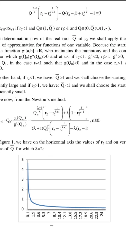
In the figure 1, we have on the horizontal axis the values of r2 and on vertical axis the value of Q for which λ=2:
Figure 1. The chart of the roots Q for the case λλλλ=2 in the case of a CES-function
0 1 2 3 4 5 0 .1 1 .9 3 .6 5 .3 7 8 .7 1 0 .4 1 2 .1 1 3 .8 1 5 .5 1 7 .2 1 8 .9 2 0 .6 2 2 .3 24
If λ→0 we know that the CES-function becomes Cobb-Douglas.
In the figure 2, we have on the horizontal axis the values of r2 and on vertical axis the value of Q for which λ=
2 1 :
Figure 2. The chart of the roots Q for the case λλλλ=
2 1
in the case of a CES-function
If λ→0 we know that the CES-function becomes Cobb-Douglas.
3. Conclusion
Considering the single real root Q of the equation: 1 r ) 1 r ( Q r r Q 1 1 2 2 1 1 2 2 1 − + − − − λ+ λ+ λ+ λ
=0 we have that: αYH>αYS if r2<1 and Q∈(0,1)∪(Q ,∞) or r2>1 and Q∈(Q ,1) that is the share from the total consumption change for Y due to the substitution effect is smaller in the case of Slutsky than in the hicksian case. Also, βYH<βYS that is the share from the total consumption change for Y due to the revenue effect is higher in the case of Slutsky than in the hicksian case.
If r2<1 and Q∈(1,Q ) or r2>1 and Q∈(0,Q )∪(1,∞) we have that αYH<αYS that is the share from the total consumption change for Y due to the substitution effect is higher in the case of Slutsky than in the hicksian case and, of course βYH>βYS that
0 0.5 1 1.5 2 2.5 0 .1 1 .6 3 4 .4 5 .8 7 .2 8 .6 10 1 1 .4 1 2 .8 1 4 .2 1 5 .6 17 1 8 .4 1 9 .8 2 1 .2 2 2 .6 24
is the share from the total consumption change for Y due to the revenue effect is smaller in the case of Slutsky than in the hicksian case.
4. References
Arrow, K.J., Chenery, H.B., Minhas, B.S. and Solow, R.M. (1961). Capital Labour Substitution and Economic Efficiency. Review of Econ and Statistics, 63, pp. 225-250.
Cobb, C.W. and Douglas, P.H. (1928). A Theory of Production. American Economic Review, 18, pp. 139–165.
Ioan, C.A. (2008). Mathematics I. Bucharest: Sinteze. Ioan, C.A. (2008). Mathematics II. Bucharest: Sinteze.
Mishra, S.K. (2007). A Brief History of Production Functions. India: North-Eastern Hill University, Shillong,
Revankar, N.S. (1971). A Class of Variable Elasticity of Substitution Production Functions. Econometrica/Econometrics, 39(1), pp. 61-71.