Moving in the Right Direction: A Regularization for Deep Metric Learning

Moving in the Right Direction: A Regularization for Deep Metric Learning

Deen Dayal Mohan*, Nishant Sankaran*, Dennis Fedorishin,

Srirangaraj Setlur, Venu Govindaraju,

Department of Computer Science and Engineering, University at Buffalo, Buffalo, New York, USA

Abstract

Deep metric learning leverages carefully designed sam-pling strategies and loss functions that aid in optimizing the generation of a discriminable embedding space. While effective sampling of pairs is critical for shaping the met-ric space during training, the relative interactions between pairs, and consequently the forces exerted on these pairs that direct their displacement in the embedding space can significantly impact the formation of well separated clus-ters. In this work, we identify a shortcoming of existing loss formulations which fail to consider more optimal di-rections of pair displacements as another criterion for op-timization. We propose a novel direction regularization to explicitly account for the layout of sampled pairs and attempt to introduce orthogonality in the representations. The proposed regularization is easily integrated into exist-ing loss functions providexist-ing considerable performance im-provements. We experimentally validate our hypothesis on the Cars-196, CUB-200 and InShop datasets and outper-form existing methods to yield state-of-the-art results.

1. Introduction

The field of metric learning has received a lot of interest in recent years. Traditionally, metric learning had been used as a method to create an optimal distance measure that ac-counts for the specific properties and distribution of the data points (for example Mahalanobis distance). Subsequently, research in metric learning has shifted to approaches that attempt to discoverrepresentationsoptimized for a specific distance measure or similarity function (euclidean distance, cosine distance, etc.). It has found application in a wide variety of tasks such as image retrieval [12], face verifica-tion [17], etc. With the advent of Deep Neural Networks, metric learning techniques have been adapted to take ad-vantage of deep non-linear transformations to obtain even more discriminative metric spaces. Popular CNNs like In-ception [19] and ResNet [6] that have been successful at

ob-*Equal contribution authors in alphabetic order

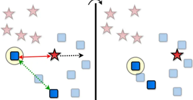
Figure 1: Difficulty of Metric Learning Optimization. Blue squares are objects of a specific class while red stars are ob-jects representing a different class. The blue square with the yellow highlight is the anchor. Greyed out objects are not considered for the loss with the current pair. A typical metric learning formulation attempts to push away embed-dings of objects belonging to different classes while moving it closer to objects having the same semantic label. How-ever, as illustrated here, such a formulation may lead to sub-optimal solutions when an object is moved closer toward an opposing cluster.

ject recognition and classification have been employed for various metric learning approaches.

Essentially, learning a metric space reduces to find-ing an embeddfind-ing space such that samples of the same class/category (positive samples) are mapped to points close to each other while ensuring that samples of different classes (negative samples) are maximally separated based on some notion of distance metric defined for the space. Out of the various formulations of this approach, one of the earliest was the Contrastive loss [3]. This loss explic-itly minimizes the distance between positive pair samples and ensures the negative pair samples are separated by a margin. Triplet loss [17] builds upon Contrastive loss by simultaneously enforcing minimization of positive pair dis-tance and maximizing negative pair disdis-tance in a single loss formulation. This requires carefully selecting ”triplets” of samples (consisting of two positive samples and a negative sample) to use for optimization to ensure that the training procedure does not get dominated by the abundance of easy

pairs available. Multi-similarity loss is one of the recent methods proposed which identifies that not all sample pairs are to be weighted the same and that the informativeness of a pair is not easily discernible from their distance/similarity alone. The loss addresses these issues by computing the rel-ative similarity amongst the positive samples and the nega-tive samples and employing it to select the pairs that would be the most beneficial for optimization.

All of the previous methods primarily focus on either de-signing a robust sampling strategy or improving the loss for-mulation by jointly considering additional distances. How-ever, one aspect that has not been explored is enforcing di-rectionduring optimization. Merely pushing the negative sample in the direction furthest away from the current sam-ple (anchor) under consideration may not be the optimal ap-proach. Fig. 1 captures one such situation where naively forcing the negative sample away from the anchor causes it to shift further into the positive cluster thereby making optimization difficult in further iterations. In this paper, we identify the necessity of incorporating the direction of repulsion as another factor for optimization and propose a new loss term that quantifies it. With this approach, we are able to discover metric spaces which are highly discrim-inable and the classes within them are better separated when compared to previous approaches. Summarizing, the main contributions of the paper are:

• identifying the importance of designing metric learn-ing objectives that jointly optimize the directions of displacement of the samples.

• proposing anovel loss criterion that explicitly moni-tors the direction of the samples being displaced and penalizes it accordingly.

• improving the performance of current state-of-the-art methods in metric learning with minimal overhead in computational complexity and parametrization.

2. Related Work

Creating a highly separable feature space using metric learning is currently an active area of research. We will focus on some recent metric learning methods to provide a context to our work, as a full overview of all methods are outside the scope of this paper.

Lecunet al. proposed [4] a siamese network with Con-trastive loss in which feature embeddings created from the input images are encouraged to be closer to each other in the feature space if the images belong to the same class and away from embeddings belonging to other classes. Triplet loss [17] incorporated a notion of relative distances be-tween feature embeddings. Lifted structure loss [14] and N-pair loss [18] improved the performance of triplet based losses by intelligently creating batches with images from

all classes, ensuring separation of the anchor from negative samples of all classes rather than a single class.

Angular loss [20] takes angle relationships between the triplets into account, for learning a stronger similarity met-ric. Yair et al. proposed proxy based metric learning[12], which avoids the computational overhead related to the cre-ation of informative triplets. Many of the metric learning methods discussed above rely on availability of informative triplets. Semi-hard negative mining [17] for face recogni-tion looks at specific triplets that violate the triplet margin constraint. The curriculum learning based approach in [1] used easier negative samples to train the network during ini-tial epochs and harder negative samples during later stages of training.

This often becomes a computationally intensive task. To alleviate this problem, [5] proposed smart mining which combines the triplet model and the global structure of the embedding space. Weighting the pairs based on the relative distance was proposed by Wuet al. [24], leading to more informative and stable samples.

Recently, ensemble methods in deep metric learning have been gaining popularity. [15] divides the last em-bedding layer of the deep network into ensembles and for-mulates training as an online gradient boosting problem. Attention-based Ensemble [8] proposed the use of multiple attention masks so that each learner can attend to different parts of the image.

None of the prior works have explicitly taken into ac-count the direction of updates during optimization.

3. Direction Regularized Metric Learning

In this section, we discuss the current approaches for deep metric learning and analyze their objectives to identify potential improvements to their formulations with the goal of improving the representation space being learnt. First, we revisit existing metric learning approaches in Section 3.1.Section3.2details the motivation and design for the new loss term incorporating directionality as a criterion.

3.1. Review of Metric Learning Approaches

Current metric learning approaches attempt to solve the optimization problem of discovering appropriate metric spaces by defining loss terms penalizing the distances be-tweenselected samples or points in the space representing assigned class centers. Typically, a standard CNN is ployed as the feature extractor that produces a feature em-beddingfxfor a given input image samplex. This feature

embedding is used for optimizing a criterion that essentially satisfies the properties listed previously.

An analysis into the design philosophies for each ap-proach would give us an insight into how they can benefit from considering not only the distances, but also the direc-tions toward which the representadirec-tions are pushed to. A

brief review of a few prominent approaches in metric learn-ing are presented below.

Triplet Loss: Schroffet al. [17] proposed Triplet loss as an augmentation over Contrastive loss [3]. Triplet loss jointly minimizes the distances between the feature embed-dings of a given sample (anchor) and another sample of the same class (positive) while maximizing the distance of the embeddings of a suitable sample of a different class (nega-tive) to the anchor. The loss is defined as below:

L= X a,p,n⊂N h kfa−fpk2− kfa−fnk2+α i + (1) The termsfa,fp,fncorrespond to feature embeddings

for the anchor, positive and negative samples, wherea, p, n

are sampled from the training datasetN.αdefines the mar-gin enforced between the anchor-negative embedding dis-tance and the anchor-positive disdis-tance. Selecting impor-tant triplets of samples is crucial and so the authors perform semi-hard negative sample mining for a particular anchor-positive sample pair in order to ensure fast convergence.

With the above formulation, the loss term pushes the negative sample radially outward with respect to the anchor sample as illustrated in Fig. 2a. However, the formulation fails to take advantage of the existence of the sampled posi-tive pair for arriving at a more optimal direction to force the negative sample to move towards.

Proxy Loss: In [12], the authors propose the use of prox-iesin place of actual samples in order to eliminate the need for sampling from a large subset of positive and negative pairs, which was identified as the limitation of the previous metric learning approaches. The proxies are “placeholder” embeddings that are statically assigned such that a single proxy embedding corresponds to a specific semantic label or class. They define the loss as:

L= X a⊂N −log e (−kfa−p(a)k2) P ne(−kfa−p(n)k 2₎ ! (2) For every sample in the dataset, the loss attempts to min-imize the distance of the anchor embeddingfato the proxy

corresponding to its classp(a)while maximizing the dis-tance of the anchor embedding to the proxies corresponding to every other classp(n). Herenindicates a negative sam-ple for the current anchora. Both the sample embeddings and proxies are learnt simultaneously during training. Even though in this formulation the optimization criterionjointly

maximizes the distances of the anchor to allthe negative classes, the lack of an explicit enforcement of an optimal direction to the negative proxies inhibits the method from achieving more efficient representations.

Multi-Similarity Loss: One of the more recent ap-proaches proposed is Multi-Similarity loss [21], which aims

to address the inadequacies of the existing loss formulations by focusing on sampling the most informative pairs for opti-mization. They accomplish this by considering the relative similarities amongst the positive samples and the negative samples in conjunction with the self-similarity measure to handle all three forms of similarities available. The loss is derived from the binomial deviance loss and is formulated as: L= 1 m m X i=1    1 αlog  1 + X p∈Pi e−α(Sip−λ)  + 1 βlog " 1 + X n∈Ni eβ(Sin−λ) # ) (3)

The firstlogterm deals with the similarity scoresSipfor

the positive samplesp∈ Piwhich comprises the set of

posi-tive data-points corresponding to theith_{anchor. The second}

log term analogously deals with that of the negative sam-ples. α, βandλare hyper-parameters. The crucial aspect here is the formation of the setsPiandNiwhich carefully

selects thehardestpositive and negative samples for the an-chor using their relative similarities. Once again, the simi-larity measure used merely optimizes the distances and di-rections originating fromindividual paircomparisons, viz., anchor-positive and anchor-negative pairs. A more thor-ough deduction of the directions of repulsion originating from other positive and negative samples in the loss term would likely yield better optimization performance.

3.2. Direction Regularization

Our review of current metric learning methods in§3.1 highlights a distinct shortcoming that we aim to correct for improving the optimization criterion. We first consider the simplest scenario involving an anchor, a positive and a neg-ative sample. Since we are dealing with a triplet of samples, the most suitable loss formulation that can be applied here is the Triplet Loss as defined in Eq. 1. To find the gradi-ents and the directions of the update for the unit normalized embeddings fa,fp,fn corresponding to the anchor,

posi-tive and negaposi-tive samples, we compute the derivaposi-tives of the loss (Eq.1) with respect to them as follows:

∂L ∂fa = 2(fn−fp) ∂L ∂fp = 2(fp−fa) ∂L ∂fn = 2(fa−fn) (4)

The above equations define the vectors used for updating the current embeddings as illustrated in Fig.2a. As seen in the figure, from this formulation during gradient descent,

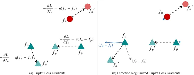
(a) Triplet Loss Gradients (b) Direction Regularized Triplet Loss Gradients

Figure 2: Behaviour of the Triplet Loss based gradient update step as compared to Triplet Loss incorporated with Direction Regularization. The samples represented by the green triangles represent a single class while the red circle represents a negative sample. The dashed black arrows indicate the update step performed on the embeddings with the computed gradients. For2b, the dotted blue arrows represent the effect of the regularization term leading to a substantial change in the wayfais

shifted as compared with the vanilla Triplet Loss.

the negative sample experiences a force in the direction of fn−fa which pushes it radially outward with respect to

fa while the positive sample is pulled towards fa with a

force offa−fp. In such a situation, we would additionally

desire to have the negative sample move in the direction orthogonal to the class cluster center ofaandpwhich we approximate asfc= fa+₂fp. Referring to Fig.3, we require

to arrive at

N C⊥P A =⇒ N C kN Ck ·

P A

kP Ak = 0 (5) Our aim is to minimize the left hand-side of the equation.

Figure 3: Geometric illustration of the layout of the anchor, positive and negative samples. The lines OA, OP and ON represent the unit-normalized embedding vectors for the an-chor (fa), positive (fp) and negative (fn) respectively. C is

the midpoint of PA and OC represents theaverage embed-ding vectorfc(not unit-normalized).

From the figure, we see that N C = fc−fn andP A =

fa−fp. Thus Eq.5becomes

(fc−fn)

kfc−fnk

· (fa−fp) kfa−fpk

= 0 (6)

Using the distributive laws of the inner product, we can expand this equation. The knowledge thatkfak=kfpk=

kfnk = 1andfc⊥P Awhich impliesfc·(fa−fp) = 0

further simplifies the equation. For a step-by-step break-down of this derivation, please refer to Appendix in the Sup-plementary materials. The equation finally becomes:

fn·fp−fn·fa= 0 (7)

Adding and subtractingfa·fa−fp·fa, we get

(fn−fa)·(fp−fa) = 1−fp·fa (8)

Now, we know that

Cos(AN, AP) =Cos(fn−fa,fp−fa)

= (fn−fa) kfn−fak

· (fp−fa) kfp−fak

(9)

Therefore, we arrive at:

Cos(AN, AP) = 1−fp·fa kfn−fakkfp−fak

(10) Hence, in order to satisfy Eq.5, we can simply minimize the cosine distance between the negative embedding w.r.t the anchor and the positive embedding w.r.t the anchor. We

denote Eq.10as thedirection regularizationterm which we apply to the standard metric loss term.

Gradient Dynamics. To understand the dynamics of minimizing Eq.10with respect to the embeddings, we inte-grate this term into the original Triplet loss formulation for a specific triplet pair and get:

Lapn=kfa−fpk 2 − kfa−fnk 2 +α −γ 1−fp·fa kfn−fakkfp−fak (11)

Here,γ is the direction regularization parameter which controls the magnitude of regularization applied to the orig-inal loss. Although having a negative regularization pa-rameter seems counter-intuitive, we must note that cosine distance ranges from [−1,+1]. Directly minimizing this term pushes its value towards−1, which leads to unfavor-able configurations where the anchor is placed between the negative and the positive sample. To avoid forming such collinearities, we minimize−Cos(AN, AP)which pushes the negative sample towards the positive quadrant of the cosine distance spectrum. As Cos(AN, AP) → 0, the negative sample is more orthogonal to the anchor-positive and the original metric loss is prioritized for optimization. WhenCos(AN, AP)→+1, the situation in Fig.2bplays out and this term acts as a penalty for the original metric loss terms and reduces the forces of displacement on the current triplet inherently performing pair weighting (as seen in the following discussion). This is also the reason for not us-ing theCos(AN, AP)term as a primary objective, rather as a penalizer that adaptively determines the contribution of the original metric loss. Taking the derivatives (step-by-step analysis can be found in the Appendix) we get the new gradient vectors as:

∂L ∂fa = 2(fn−fp)−γc(fa−fp)−γdk(fn−fa) ∂L ∂fp = 2(fp−fa)−γc(fp−fa) ∂L ∂fn = 2(fa−fn)−γc d(fa−fn) (12) The terms c = (kfn−fakkfa−fpk)−1,d = kfn−

fak−2 andk = kfn −fak−1kfa−fpkare scaling

fac-tors that adaptively control the contributions of the gradients they are paired with.cspecifically looks at the relative dis-tances of the negative and positive embeddings (w.r.t the an-chor). The value ofcis highest only if both the negative and positive embeddings aresimilarlyvery close to the anchor. In this case the term γc(fa −fp)in ∂∂fLa exerts a greater force on fa in the direction leading away from the

nega-tive embedding as compared to the previous formulation in Eq.4, thereby prioritizing increasing the gap between itself and the negative sample (see Fig. 2b). However, the third

termγdk(fn−fa)also dominates owing to a highdkvalue

(negative close to anchor) and there is a force acting onfa

to move closer tofn so as to decrease the cosine

similar-ity of< fa−fn,fa −fp >. Instead of naively moving

towardsfp, it tries to re-position itself such that the

nega-tive sample is orthogonal to the anchor-posinega-tive pair. Note that in the original Triplet loss, though the anchor is shifted away from the negative sample, it attempts to move closer to the positive sample. It doesn’t account for the fact that the positive may be located close to the negative sample, in which case the displacement of the anchor is sub-optimal. The direction regularization term in our formulation effec-tively addresses this issue.

Interestingly, when considering _∂∂_fL

p, we find that for high c values, the effect of the gradient on fp is

dimin-ished by a factor ofγc. This seems counter-intuitive at first, but we see that in such a situation with the negative sam-ple being close to both anchor and positive samsam-ples, this specific triplet is not as informative for deducing the final positions of the anchor and positive embeddings and hence downplays the contribution of the gradient vector arising from this specific triplet. Note that this weighting is done inherently as part of the loss formulation and does not re-quire any external supervision to implement it (for exam-ple manually evaluating the available triexam-plets for informa-tiveness). The gradient of negative embeddingfn behaves

similar to the original Triplet loss, unless the negative sam-ple is very close to the anchor, in which case the negative sample would not be shifted significantly owing to the loss formulation assigning the current triplet pair as being un-informative. The reason being that, in such a situation, it may be unclear whether the anchor sample is currently an outlier located in the region of the space occupied by other negative samples or conversely if the negative sample is the outlier in a field of positive samples. Overall, the proposed direction regularization inherently computespair weighting

based on the forces acting upon the current sample set and hence leads to the system mining for more informative ex-amples to update the embedding space if the current set is deemed unfit.

3.3. Adapting Metric Learning Losses with

Direc-tion RegularizaDirec-tion

In the previous sections, we analyzed the effect of in-cluding the proposed direction regularization term into the loss formulation. We observe that the system dynamically modifies the gradient vector in accordance with the layout of the current sampling of anchor, positive and negative samples. As we have highlighted in§3.1, since current met-ric learning losses lack an explicit enforcement of orthog-onality of the negative sample with respect to the anchor-positive pair, it would be beneficial to imbue the properties of direction regularization into their formulations to make

them robust. The following definitions provide an intuition and develop a guide to easily adapt the regularization term into any standard metric learning loss function.

Triplet Loss: Given that we have already described an adaptation of the Triplet loss in the previous section, we can rewrite Eq.11to be more readable:

Lapn=kfa−fpk 2 − kfa−fnk 2 +α −γ Cos(fn−fa,fp−fa) (13)

Proxy Loss. With respect to Proxy loss, we note that the loss formulation considers a single anchor embedding, a single proxy embedding corresponding to the class of the anchor as the positive sample andnproxy embeddings for all other classes as negative samples. Since the direction regularization term computes Cos(AN, AP)with the an-chor and positive proxy being fixed, there arensuch terms for thennegative proxies. Hence we include it alongside the negative proxy distance term in Eq.2to get:

L= X a⊂N −log e (−kfa−p(a)k2) P ne[−kfa−p (n)k2_{−γ Cos(p(n)−f} a,p(a)−fa)] ! (14)

Multi-Similarity Loss. Similar to Proxy loss, since the negative samples chosen are with respect to a particular an-chor and the hardest positive sample, we include the regu-larization term in the negative sample distances in Eq.3and obtain: L= 1 m m X i=1    1 αlog  1 + X p∈Pi e−α(Sip−λ)  + 1 β log " 1 + X n∈Ni eβ(Sin−λ−γ Cos(fn−fa,fp−fa)) # ) (15)

4. Experiments

For all experiments, we use GoogLeNet [19] with batch normalization [7] in order to present a fair comparison with other methods. The network which is pre-trained on ILSVRC 2012-CLS [16] is fine-tuned on each of the below mentioned datasets respectively. All images were cropped to224×224and standard preprocessing techniques are ap-plied. Data is augmented with random crop and random horizontal flipping for training, and center crop for testing. Adam [9] is used as the optimizer.

We perform experiments on three standard datasets: CUB-200-2011 [23], Cars-196 [10], and In-Shop Clothes Retrieval [11].

4.1. CUB-200-2011

The Caltech-UCSD CUB-200-2011 dataset features 11,788images of classes of fine-grained bird species across 200classes. The first100classes (5,864images) are used for training, and the remaining100classes (5,924images) for testing.

4.2. Cars-196

The Cars-196 dataset has 16185images in 196classes of car models. Each class represents amake, model, year

triple, for example, 2012 Tesla Model S. The first98classes (8,054 images) are used for training, with the remaining classes (8,131images) used for testing.

4.3. In-Shop Clothes Retrieval

In-Shop Clothes Retrieval (In-Shop) is a large-scale clothing retrieval dataset with52,712images across7,982 classes (clothing items). 25,882 images in3,997 classes are used for training, and 14,218 and12,612 images in the remaining3,985classes are used for the test query and gallery sets, respectively.

4.4. Comparison with the state-of-the-Art

We compare the performance of the proposed models to other methods on the three datasets. We use the direction regularized version of MS-Loss and fix an embedding di-mension of 64 for experiments on the Caltech-UCSD CUB-200-2011 and Cars-196 and 512 for experiments on the In-Shop Clothes Retrieval dataset. The hyper parameters in Eq.15α,β,λare set as2,50and0.7respectively. The pa-rameterγis learned during training. We report performance using the standard Recall@K metric.

Table 1: Evaluation on CUB-200-2011 Dataset

Recall@K (%) 1 2 4 8 Triplet Semihard [17] 42.6 55.0 66.4 77.2 Lifted Struct [14] 43.6 56.6 68.6 79.6 Clustering64 [13] 48.2 61.4 71.8 81.9 Npairs [18] 51.9 64.3 74.9 83.2 Angular [20] 54.7 66.3 76.0 83.9 Proxy NCA64[12] 49.2 61.9 67.9 72.4 Margin128 [24] 63.6 74.4 83.1 90.0 HDC384 [13] 53.6 65.7 77.0 85.6 HDML512[25] 53.7 65.7 76.7 85.7 RLL512[22] 57.4 69.7 79.2 86.9 MS64 [21] 57.4 69.8 80.0 87.8 DR-MS64 59.1 71.0 80.3 87.3 DR-MS512 66.1 77.0 85.1 91.1

From Table1and Table2, we note that the our method outperforms all the other methods on the fine grained datasets Caltech-UCSD CUB-200-2011 and Cars-196. We obtain nearly a2%increase in Recall@1 compared to MS-Loss and a10%increase in Recall@1 compared to Proxy-NCA. An interesting observation is that the increase in per-formance for Recall@1 compared to other methods is with an embedding dimension of 64. This can be attributed to a couple of factors: 1) The directional regularization enforced

Table 2: Performance on Cars-196 Dataset Recall@K (%) 1 2 4 8 Triplet Semihard[17] 51.5 63.8 73.5 81.4 Lifted Struct[14] 53.0 66.7 76.0 84.3 Clustering64 [13] 58.1 70.6 80.3 87.8 Npairs[18] 71.1 79.7 86.5 91.6 Angular[20] 71.4 81.4 87.5 92.1 Proxy NCA64 [12] 73.2 82.4 86.4 88.7 Margin128[24] 79.6 86.5 91.9 95.1 HDC384[13] 73.7 83.2 89.5 93.8 HDML512 [25] 79.1 87.1 92.1 95.5 RLL512 [22] 74.0 83.6 90.1 94.1 MS64[21] 77.3 85.3 90.5 94.2 DR-MS64 79.3 86.7 91.4 94.8 DR-MS512 85.0 90.5 94.1 96.4

Table 3: Performance on In-Shop Dataset

Recall@K (%) 1 10 20 30 40 50 HDC384 [13] 62.1 84.9 89.0 91.2 92.3 93.1 ABIER512[15] 83.1 95.1 96.9 97.5 97.8 98.0 ABE512[8] 87.3 96.7 97.9 98.2 98.5 98.7 FastAP512 [2] 89.0 97.2 98.1 98.5 98.7 98.9 MS128 [21] 88.0 97.2 98.1 98.5 98.7 98.8 MS512[21] 89.7 97.9 98.5 98.8 99.1 99.2 DR-MS512 91.7 98.1 98.7 98.9 99.1 99.2

by the proposed method can help in finding superior direc-tions to which the samples are to be moved in order to create better separation in such low dimensions. 2) Due to the in-herent pair weighting of samples as explained in Section3 there is a stricter constraint on the samples during the po-sitional updates. When using embedding dimension of 512 we significantly outperform other methods by a substantial margin.

Additionally from Table3we see that our method scales well to datasets with a larger number of classes to out-perform other methods on the In-Shop Clothes Retrieval dataset. We obtain nearly a 2% improvement over the current state-of-the-art MS-Loss. In the qualitative analy-sis (Fig4), we see that for Recall@5 results, the DR-MS method is able to correctly select the true-positive samples (red border) during retrieval as opposed to the standard MS loss.

Analyzing the value ofγlearned during training, we note thatγtakes positive values further validating our theoretical analysis.

4.5. Ablation Study

In order to experimentally validate our proposed method, we compare our direction regularized methods from Eq.13, 14and15with the corresponding original versions of these

methods on the Caltech-UCSD CUB-200-2011 dataset. We selected the Proxy-NCA loss in addition to the Triplet and MS losses in order to study the effect of the direction reg-ularization on sampling-free methods as well. We fix an embedding dimension of 64 for the experiments and report performance using the standard Recall@K metric as shown in table4.

Table 4: Ablation study to show the effect of direction regu-larization when applied to standard metric learning methods on CUB-200 dataset. ’*’ indicates a re-implementation of original version Recall@K (%) 1 2 4 8 Triplet Loss* 51.9 64.0 70.3 74.1 DR-Triplet Loss 54.2 66.1 72.5 77.0 Proxy-NCA 49.2 61.9 67.90 72.4 DR-Proxy-NCA 53.8 65.7 75.8 84.6 MS 57.4 69.8 80.0 87.8 DR-MS 59.1 71.0 80.3 87.3

A newer version of GoogLeNet with batch normaliza-tion is used for implementing Triplet loss. We do not use any sample mining strategy in both the Triplet loss and the direction regularized version. We fix the hyper-parameterγ

in Eq.13to 0.45.

The multi-similarity based triplet sampling strategy pro-posed in [21] is used for both MS-Loss and our direction regularized version.αandβare set to2and50respectively in Eq.3.

As can be seen from Table1, our direction regularized loss functions outperform the corresponding vanilla ver-sions. The performance with the original loss formulation clearly suffers from the sub-optimal directions in which the samples are separated during optimization. Moreover, with the performance improvement over corresponding versions of Triplet Loss and MS-Loss, it is interesting to note that our direction based regularization results in improvement agnostic of whether or not a sampling strategy is used. Table 5: Effect on recall performance with respect to vari-ation in the influence of the direction regularizvari-ation (con-trolled byγ) and variation in training batch size.

Recall@K (%) 1 γ= 0.0 57.4 γ= 0.1 58.7 γ= 0.2 59.1 γ= 0.3 60.5 γ= 0.4 57.0 Learnableγ 59.1

(a) Performance for differ-entγon CUB-200 Dataset

Recall@K (%) 1

80 87.4

160 88.3

320 89.5

600 91.7

(b) Performance for different batch sizes on In-Shop Dataset

Figure 4: Recall@5 Qualitative results on the CUB-200-2001 dataset comparing the proposed DR-MS loss performance with MS-Loss [21]. Images with a red border indicate the true positive gallery images for the given query image which DR-MS is able to correctly identify in its top-5 results whereas MS is not able to.

Our proposed method provides a trivial way of incorpo-rating direction regularization into existing metric learning functions and thereby regulating the direction in which the samples are separated. This helps in creating a stronger em-bedding separability, leading to better performance.

4.6. Regularization Factor vs Performance

To understand the behavior of the metric learning system when varying the degree of direction regularization applied to the loss, we conduct experiments on different values of the regularization factor γ. The embedding dimension is set to 64. Table 5ashows performance variations for cer-tain choices of γ and it is seen that the best performance on the CUB-200 dataset is achieved with a γ = 0.3. We notice that the performance obtained by the system when

γis a learnable parameter is slightly diminished compared to when a staticγ = 0.3 is used. However, despite using a learnable γwe are able to see a substantial enough per-formance boost when compared to the non-regularized MS-loss (γ = 0). The performance starts drastically reducing when settingγ ≥ 0.4 as the regularization term begins to overpower the metric loss’ contribution and meaningful em-beddings are harder to discover under such strict constraints of the direction regularization. From these analyses, we can conclude that, in general, picking aγvalue in the range of [0.2,0.4)(under the current experimental setting) seems to provide the best performance improvements.

4.7. Batch Size vs Performance

We study the variation in performance of MS-Loss hav-ing direction regularization with different batch sizes. We

perform the experiment on the In-Shop dataset since it is a larger set compared to Caltech-UCSD CUB-200-2011 and will help us form a better understanding of the results. We use a learnableγand fix the embedding size to 512. As is seen in Table5b, we find that performance increases with batch size. This can be attributed to the fact that a larger batch size helps in identifying more informative triplets.

5. Conclusion

Deep metric learning attempts to solve the challenging task of creating rich representation spaces that encode the intra-class diversity while maintaining a clear separation be-tween classes. The discovery of such spaces is extremely sensitive to the path chosen during optimization. Intelli-gent updates to the sample embeddings by making judicious use of all the information available in the neighbourhood of samples is crucial. In this work, we have identified an in-adequacy in the existing metric learning loss formulations in their lack of consideration of the optimal direction of up-date. Our proposed solution corrects for this by introducing a novel direction regularization factor that compels the pairs towards the most suitable positions in the metric space. In doing so, the loss function inherently implements a form of pair weighting based off of the gradients originating from the relative distribution of the positives and negatives with respect to the anchor. The method achieves state-of-the-art results on standard image retrieval datasets and conse-quently validates the need for such a regularization factor in the loss formulations.

References

[1] Srikar Appalaraju and Vineet Chaoji. Image similarity using deep cnn and curriculum learning. arXiv preprint arXiv:1709.08761, 2017.2

[2] Fatih Cakir, Kun He, Xide Xia, Brian Kulis, and Stan Sclaroff. Deep metric learning to rank. InProceedings of the IEEE Conference on Computer Vision and Pattern Recogni-tion, pages 1861–1870, 2019.7

[3] S Chopra. Learning a similarity metric discriminatively, with application to face verification. In IEEE Conference on Compter Vision and Pattern Recognition, pages 539–546, 2005.1,3

[4] Raia Hadsell, Sumit Chopra, and Yann LeCun. Dimensional-ity reduction by learning an invariant mapping. In2006 IEEE Computer Society Conference on Computer Vision and Pat-tern Recognition (CVPR’06), volume 2, pages 1735–1742. IEEE, 2006.2

[5] Ben Harwood, BG Kumar, Gustavo Carneiro, Ian Reid, Tom Drummond, et al. Smart mining for deep metric learning. In

Proceedings of the IEEE International Conference on Com-puter Vision, pages 2821–2829, 2017.2

[6] Kaiming He, Xiangyu Zhang, Shaoqing Ren, and Jian Sun. Deep residual learning for image recognition. In Proceed-ings of the IEEE conference on computer vision and pattern recognition, pages 770–778, 2016.1

[7] Sergey Ioffe and Christian Szegedy. Batch normalization: Accelerating deep network training by reducing internal co-variate shift.arXiv preprint arXiv:1502.03167, 2015.6

[8] Wonsik Kim, Bhavya Goyal, Kunal Chawla, Jungmin Lee, and Keunjoo Kwon. Attention-based ensemble for deep met-ric learning. InProceedings of the European Conference on Computer Vision (ECCV), pages 736–751, 2018.2,7

[9] Diederik P Kingma and Jimmy Ba. Adam: A method for stochastic optimization. arXiv preprint arXiv:1412.6980, 2014.6

[10] Jonathan Krause, Michael Stark, Jia Deng, and Li Fei-Fei. 3d object representations for fine-grained categorization. In

Proceedings of the IEEE International Conference on Com-puter Vision Workshops, pages 554–561, 2013.6

[11] Ziwei Liu, Ping Luo, Shi Qiu, Xiaogang Wang, and Xi-aoou Tang. Deepfashion: Powering robust clothes recog-nition and retrieval with rich annotations. InProceedings of IEEE Conference on Computer Vision and Pattern Recogni-tion (CVPR), June 2016.6

[12] Yair Movshovitz-Attias, Alexander Toshev, Thomas K Le-ung, Sergey Ioffe, and Saurabh Singh. No fuss distance met-ric learning using proxies. InProceedings of the IEEE In-ternational Conference on Computer Vision, pages 360–368, 2017.1,2,3,6,7

[13] Hyun Oh Song, Stefanie Jegelka, Vivek Rathod, and Kevin Murphy. Deep metric learning via facility location. In Pro-ceedings of the IEEE Conference on Computer Vision and Pattern Recognition, pages 5382–5390, 2017.6,7

[14] Hyun Oh Song, Yu Xiang, Stefanie Jegelka, and Silvio Savarese. Deep metric learning via lifted structured fea-ture embedding. InProceedings of the IEEE Conference

on Computer Vision and Pattern Recognition, pages 4004– 4012, 2016.2,6,7

[15] Michael Opitz, Georg Waltner, Horst Possegger, and Horst Bischof. Deep metric learning with bier: Boosting inde-pendent embeddings robustly.IEEE transactions on pattern analysis and machine intelligence, 2018.2,7

[16] Olga Russakovsky, Jia Deng, Hao Su, Jonathan Krause, San-jeev Satheesh, Sean Ma, Zhiheng Huang, Andrej Karpathy, Aditya Khosla, Michael Bernstein, et al. Imagenet large scale visual recognition challenge. International journal of computer vision, 115(3):211–252, 2015. 6

[17] Florian Schroff, Dmitry Kalenichenko, and James Philbin. Facenet: A unified embedding for face recognition and clus-tering. InProceedings of the IEEE conference on computer vision and pattern recognition, pages 815–823, 2015. 1,2,

3,6,7

[18] Kihyuk Sohn. Improved deep metric learning with multi-class n-pair loss objective. InAdvances in Neural Informa-tion Processing Systems, pages 1857–1865, 2016.2,6,7

[19] Christian Szegedy, Wei Liu, Yangqing Jia, Pierre Sermanet, Scott Reed, Dragomir Anguelov, Dumitru Erhan, Vincent Vanhoucke, and Andrew Rabinovich. Going deeper with convolutions. InProceedings of the IEEE conference on computer vision and pattern recognition, pages 1–9, 2015.

1,6

[20] Jian Wang, Feng Zhou, Shilei Wen, Xiao Liu, and Yuanqing Lin. Deep metric learning with angular loss. InProceedings of the IEEE International Conference on Computer Vision, pages 2593–2601, 2017. 2,6,7

[21] Xun Wang, Xintong Han, Weilin Huang, Dengke Dong, and Matthew R Scott. Multi-similarity loss with general pair weighting for deep metric learning. InProceedings of the IEEE Conference on Computer Vision and Pattern Recogni-tion, pages 5022–5030, 2019.3,6,7,8

[22] Xinshao Wang, Yang Hua, Elyor Kodirov, Guosheng Hu, Romain Garnier, and Neil M Robertson. Ranked list loss for deep metric learning. arXiv preprint arXiv:1903.03238, 2019.6,7

[23] P. Welinder, S. Branson, T. Mita, C. Wah, F. Schroff, S. Be-longie, and P. Perona. Caltech-UCSD Birds 200. Technical Report CNS-TR-2010-001, California Institute of Technol-ogy, 2010.6

[24] Chao-Yuan Wu, R Manmatha, Alexander J Smola, and Philipp Krahenbuhl. Sampling matters in deep embedding learning. InProceedings of the IEEE International Confer-ence on Computer Vision, pages 2840–2848, 2017.2,6,7

[25] Wenzhao Zheng, Zhaodong Chen, Jiwen Lu, and Jie Zhou. Hardness-aware deep metric learning. InProceedings of the IEEE Conference on Computer Vision and Pattern Recogni-tion, pages 72–81, 2019.6,7