Fitting cornering speed models with one-class support vector machines

Fitting Cornering Speed Models with

One-Class Support Vector Machines

James M. Fleming

Xingda Yan

Roberto Lot

University of Southampton, UK

Abstract—This paper investigates the modelling of cornering speed using road curvature as a predictive variable, which is of interest for advanced driver assistance system (ADAS) applications including eco-driving assistance and curve warning. Such models are common in the driver modelling and human factors literature, yet lack reliable parameter estimation methods, requiring an ad-hoc evaluation of the upper envelope of the data followed by linear regression to that envelope. Considering the space of possible combinations of lateral acceleration and cornering speed, we cast the modelling of cornering speed as an ‘outlier detection’ problem which may be solved using one-class Support Vector Machine (SVM) methods from machine learning. For an existing cornering model, we suggest a fitting method using a specific choice of kernel function in a one-class SVM. As the parameters of the cornering speed model may be recovered from the SVM solution, this provides a more robust and reproducible fitting method for this model of cornering speed than the existing envelope-based approaches. In addition, this gives comparable outlier detection performance to generic SVM methods based on Radial Basis Function (RBF) kernels while reducing training times by a factor of 10, indicating potential for use in adaptive eco-driving assistance systems that require retraining either online or between drives.

I. INTRODUCTION

It is of considerable interest to be able to predict the speed at which a driver will negotiate a curve based on values which may be readily estimated from mapping services, such as road curvature, as this has several useful applications to Advanced Driver Assistance Systems (ADAS). The authors’ main motivation in investigating this problem is to build predictive models of cornering speed for eco-driving assistance systems, which are designed to save fuel and emissions by coaching the driver to coast down and to avoid braking before corners and intersections [1]. Another potential application is in curve warning systems, which rely on estimates of the speed at which a driver will take a corner in order to identify when a warning is required [2]. Such systems may be particularly useful to riders of motorcycles, as a relatively high proportion of motorcycle accidents are due to rider error in curves [3].

More generally, ADAS that adapt to driver behaviour may be beneficial for improved user acceptance and better out-comes in both fuel-saving and safety applications. This can be achieved by estimation of the parameters of some model of the driver’s behaviour, which may be carried out online or between journeys. Such adaptive ADAS have been explored in the context of collision warning and adaptive cruise control systems [4]. Methods for estimation of parameters of longitu-dinal models of driver behaviour, such as the Intelligent Driver

Model (IDM) of vehicle-following [5], are already available, for example by minimisation of the least-squares error [6] or Kalman filtering performed online [7]. In contrast, there has been little work on parameter fitting methods for models of cornering speed, forming a gap in the current literature.

Existing models of cornering speed often take the form of an inequality relating either speed and road curvature or speed and lateral acceleration, precluding the use of least-squares fitting methods unless some (normally subjective) identification of the envelope of the data is made first. In this paper, we propose that models of this type may be fit more robustly and repeatably by employing one-class SVM techniques for outlier detection from the machine learning literature, and we illustrate this by providing a parameter fitting method for the ‘lateral acceleration margin’ model of cornering speed given by Reymond et al. in [8]. Similar one-class SVM techniques have already been suggested for use in ADAS, in particular for collision warning systems based on measurements of time-to-collision [9]. Viewing the prob-lem as one of ‘one-class classification’ is natural for ADAS applications involving cornering since real-world driving data contains many examples of ‘normal’ or ‘acceptable’ cornering speeds but, by definition, very few examples of ‘abnormal’ or ‘outlier’ cornering speeds that are of interest to the ADAS. With the potential curve warning application in mind, we compare the performance of the fitted model as a classifier to generic kernel SVM methods based on Radial Basis Functions (RBFs). For eco-driving assistance, in which a closed-form predictive model of cornering speed is required, we provide formulae to calculate the parameters of the model of [8] in terms of the one-class SVM solution.

II. LITERATUREREVIEW A. Models of cornering speed

Early studies on driver cornering speed behaviour concen-trated on lateral acceleration as sensed by the human vestibular system as the perceived quantity limiting speed in curves, with it being noted as early as 1968 that drivers choose lower lateral accelerations at higher speeds [10]. Later work confirmed this effect and attempted to model the relationship empirically, finding a nonlinear relationship [11]. From dynamics, the lateral acceleration while traversing a path of curvatureκ, or equivalently of curvature radiusR, is given by

alat=κv2= v2

where v is the forward velocity along the path. For a driver following a road the path may be considered fixed. In that case, an upper bound on the lateral acceleration the driver will tolerate then implies a maximum tolerable speed for each curve. This has been confirmed empirically, with curvature found to the be the predominant factor affecting speed choice on curves on rural roads when drivers are not constrained by other factors such as signage [12], [13].

From experiments performed in a fixed-base driving sim-ulator (in which the effects of lateral acceleration cannot be felt by the driver), [14] identified that the amount of time until the vehicle crosses the lane marking on the outside-edge of the lane is approximately constant for curves of different curvatures. This forms a quantity known as time-to-lane crossing (TLC) that, by visual feedback, is kept above a certain minimum threshold by drivers negotiating a curve. This quantity has also been shown to be important in lane-change manoeuvres [15]. If steering error is assumed to increase when negotiating curves of larger curvature, a lower bound on TLC also implies a lower cornering speed for tighter curves.

The link between these apparently different viewpoints of vestibular versus visual feedback was given by Reymond et al. in the appendix to [8], which shows that for a curve radius

R and the assumption of some small steering error, the TLC satisfies the relationship

TLC∝ R

1/2

v (2)

so that a lower bound on TLC implies an upper bound to the lateral acceleration (1). This led the authors to postulate a mar-gin of error of the driver when estimating the curvature of an upcoming corner, implying a decreasing quadratic relationship between the upper bound of lateral acceleration and vehicle velocity. Denoting road curvature by κ and cornering speed by v, this implies a bound on lateral acceleration given by

alat =κv2≤Γmax−∆Cmaxv2 (3)

in which Γmax is a parameter representing the maximum

desirable lateral acceleration value and ∆Cmax is the error

margin for curvature estimation. This relationship was veri-fied experimentally in both a simulator and on a test track. To estimate these parameters for drivers, [8] uses a two-step process of estimating the upper envelope of the lateral acceleration when plotted against speed, and then performs a linear regression to this envelope. This method is also used to fit the same model in [16], which compares it to the hypothesis of a constant TLC and other models.

To obtain the implied relationship of the model between curvature and maximum cornering speed, we may rearrange (3) to find v≤ r Γmax κ+ ∆Cmax (4) from which it is clear that maximum velocity decreases as road curvature increases, with an overall limit on velocity for

κ= 0 given by v ≤q Γmax

∆Cmax. The particular values of Γmax

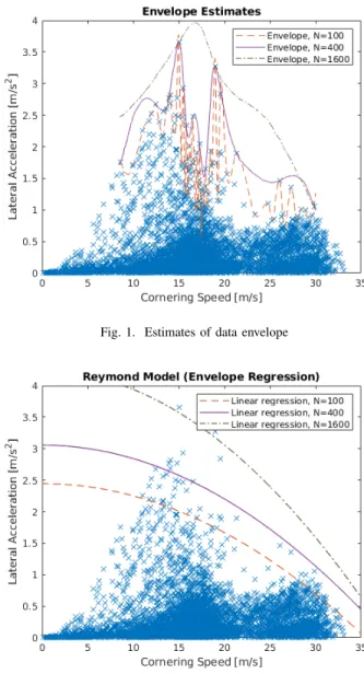
Fig. 1. Estimates of data envelope

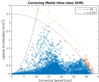
Fig. 2. Lat. accel. margin model, fit to envelopes

and ∆Cmax vary between drivers. For example, it is noted

in [8] that a trained test driver had a higher value of Γmax

and significantly lower value of∆Cmax than the other drivers

involved in the study.

B. Problems with envelope-based parameter estimation In this section, we note some shortcomings of the approach of estimating the upper envelope of lateral acceleration data and using this to perform a linear regression, which motivates the fitting procedure developed in the remainder of the paper. In [8] the envelope was estimated subjectively by inspection of the data, but we consider a computational approach similar to [17] which estimates the upper tangent points of the envelope and then fits an interpolating spline to these points. This is implemented in theenvelopefunction in the Matlab Signal Processing toolbox using the ‘peaks’ option for the algorithm. This function also includes a parameter, N, such that the points chosen for interpolation are local maxima of the data

Γmax[m/s2] ∆Cmax[rad/km]

N= 100 2.45 1.94

N= 400 3.06 2.13

N= 1600 4.23 2.93 TABLE I

VALUES OF FITTED PARAMETERS,ENVELOPE METHOD

with a separation of at least N points between successive interpolation points. The results of applying this to determine the upper envelope are shown in Figure 1 for varying values of

N. Depending upon the smoothness required for the envelope, it can be seen that quite different curves are obtained. The endpoints of the envelopes are chosen to be at9m/s and30m/s. Although it is not apparent from the figure, the resulting curves also vary depending on this choice of endpoints.

These envelopes were then used to determine Γmax and

∆Cmaxof (3) by linear regression, following the method given

in [8]. The results are shown in Figure 2 and Table I for the different values of N, and it is apparent that different choices of envelope lead to very different fitted curves and parameters. In fact, for repeatability we must specify not only the value of N, but also those of the endpoints, and the resulting variation in the fitted parameters is considerable even for small changes in these values. In addition, there is no reason to believe that the obtained curve generalises well when more data is collected, with no a priori indication of the number of measurements expected to be outliers and fall outside the fitted curve. This motivates us, in the following sections, to develop an alternative method that is more robust and repeatable, considering all the data points rather than only the ones on the envelope and requiring the specification of only a single parameter for repeatability. By basing this method on the theory of one-class classification from machine learning, we can also specify ahead of time the proportion of measurements expected to fall outside the fitted curve.

III. METHODS A. Data collection

Real-world cornering data was collected as part of a small-scale driving study, carried out as part of the G-ACTIVE research project (http://www.g-active.uk) at the University of Southampton in the UK. The data was collected over a series of drives from a participant who had a daily commute through a rural area and who contributed a total of 10 hours of data over 17individual drives, mostly in rural conditions in which speed was not limited by other traffic. Time-series data from GPS was analysed by extracting all local curvature maxima and the corresponding observed velocity, giving a total of 7384 cornering events that we denote by a pair (vi, ai) of cornering speed and lateral acceleration values. For more detailed information on the collection and processing of this cornering data, we refer readers to [18], which describes the data processing and analysis, and [19], which describes the data collection device used.

B. One-class SVM classifiers

The one-class SVM approach that we use was developed in [20], and consists of solving the Quadratic Program (QP)

minimise w∈F, ξ∈Rl, ρ∈R 1 2kwk 2₊ 1 lν X i ξi−ρ subject to w·Φ(xi)≥ρ−ξi, ξi≥0 ∀i (5)

in which xi represents the data points in some training set, l is the number of such points, Φ(·) is a mapping of those points to a feature space used for classification, w andρare decision variables that will define the classifier, and theξiare slack variables associated with the constraintw·Φ(xi)≥ρ. Noting that the sum of these slack variables is penalised in the cost function, so we may expect that for the solutionw∗,

ρ∗we havew∗·Φ(xi)≥ρ∗for mostxi, so that this specifies some region containing most of the data. The parameterν has the useful interpretation as an upper bound on the proportion of outliers in the training set [20].

Rather than solving 5 directly, it is more common to solve the Lagrange dual, which may be expressed as the QP

minimise α∈Rl 1 2 X i X j αiαjk(xi,xj) subject to 0≤αi≤ 1 lν ∀i, X i αi= 0 (6)

in which we have introduced the kernel function:

k(x,y) = Φ(x)·Φ(y) (7) This has the advantage that k(x,y)may sometimes be much faster to calculate thanΦ(x)·Φ(y). For classification purposes, we may recoverw∗ andρ∗ from the solutionsα∗_i using

w∗=X i

α∗_iΦ(xi) (8)

and, for anyisuch that0< αi< _lν1:

ρ∗=w∗·Φ(xi) (9)

By introducing different kernel functionsk(·,·), various non-linear classifiers may be constructed. Common choices are the polynomial kernels k(x,y) = (x·y+c)d _{for c ≥ 0 and} some integer d, or the Radial Basis Function (RBF) kernel

k(x,y) = exp(−kx₂−_σy2k2) for someσ≥0, which we use for

comparison purposes later in the present paper. C. One-class SVMs for cornering models

For each corner, we assume that we have measurements of lateral accelerationai and cornering speedvi available. We would like to find some region of the(v, a)-space that contains a high proportion,1−ν, of the points(vi, ai)so that abnormal values may be identified, for example when approaching a corner at excessive speed for a curve warning system. This is an ‘outlier detection’ problem that is naturally handled by the one-class classification methods already discussed, in that data for the ‘abnormal’ values of(v, a)is typically unavailable

while a large quantity of ‘normal’ values(vi, ai)are available for model fitting.

To develop a fitting method for the safety-margin model (3), we consider the simple feature mappingΦ : (vi, ai)→(vi2, ai) and the primal form of the one-class SVM (5). This squaring of the velocity is likely to lead to large values that lead to poor scaling of the problem, so we additionally standardise the predictors by introducing scaled and centred variables

yi= v2 i −µv2 σv2 (10) and zi= ai−µa σa (11) whereµandσrepresent the usual sample mean and standard deviation respectively. We therefore obtain the QP problem

minimise ξ∈Rl, w1,w2,ρ∈R w2 1 2 + w2 2 2 + 1 lν X i ξi−ρ subject to w1yi+w2zi≥ρ−ξi, ξi≥0 ∀i w1≤0, w2≤ −ε2 (12)

which is a modification of the standard one-class SVM (5) in which the variables w1 and w2 are constrained to be

nonpositive and negative respectively via the use of a small parameter ε. In many cases, these constraints on w1 and w2

may be omitted without altering the solution, but we include them to ensure that the fitted decision boundary represents an upper bound on lateral acceleration that decreases with increasing v, regardless of the data (vi, ai). As before, ν denotes an upper bound on the desired proportion of outlier measurements in the training data, and the penalisation of the slack variables ξi in the cost function ensures that the constraintw∗₁yi+w∗2zi≥ρ∗ holds in the solutionw1∗,w∗2,ρ∗

for at least 1−ν of the training values(vi, ai).

Comparing coefficients with the safety-margin model (3) and noting that w∗₂<0, we see that for these two constraints to be equivalent requires Γmax=µa+σa ρ∗ w∗ 2 +σa µv2 σv2 w₁∗ w∗ 2 (13) and ∆Cmax=σa µv2 σv2 w∗₁ w∗₂ (14)

so that we may consider (12) as a parameter fitting procedure for this model ensuring that at least1−νof the training values

(vi, ai)satisfy the inequality (3).

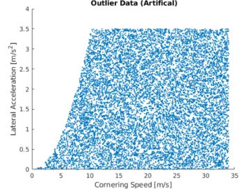
Examples of the results when using the preceding method to fit (3) are shown in Figure 3, which takes ν = 0.1% and ν = 1%. This figure also shows the line given by

a =κmaxv2 which represents a physical upper bound on the

lateral acceleration based on the maximum cornering curvature

κmax of the vehicle used for data collection. As expected,

fewer points lie below the curve as ν is increased, and for given data (vi, ai)the fitting procedure is entirely repeatable for a given value of ν. We also compare this approach with the one-class SVM optimisation of (5) using the RBF kernel

Fig. 3. Lat. accel. margin model, SVM fit to training data. The black dash-dotted line shows the cornering capability of the vehicle

Fig. 4. RBF Kernel SVM, fit to training data

k(x,y) = exp(−kx₂−_σy2k2), for which the resulting decision

boundaries are shown in Figure 4 using the same training data. D. Data analysis and testing

We now consider the application of the one-class SVM pro-cedures to the outlier detection problem as required for a curve warning system. The data were split into Training, Validation and Test subsets with approximately 70%, 10% and 20% in each subset respectively. Two techniques were used to fit to the data in the Training set, the one-class SVM optimisation of (5) using the RBF kernel k(x,y) = exp(−kx₂−_σy2k2), and

the safety-margin model (3) using the optimisation of (12) with the model parameters recovered using (13) and (14). This was carried out using the fitcsvm function in the Matlab Statistics and Machine Learning toolbox in each case. The validation subset was used to choose the scaling factor for the Gaussian kernel used in the kernel SVM by choosing the

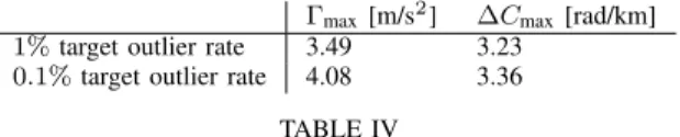
Fig. 5. Artificial outlier data for testing

kernel size that gave the lowest misclassification rate over the validation data.

For testing purposes, it is useful to generate some artificial data that can be treated as a second ‘outlier’ class to evaluate the performance of the one-class classifier over the testing subset. This is necessary as it is difficult to obtain true data for this outlier class, as it would correspond to rare instances in which the driver took a corner at a high and possibly unsafe speed. The artificial outlier data generated is shown in Figure 5 and consists of samples from a uniform distribution over the space of possible cornering speed and lateral acceleration combinations, excluding cases for whichalat> kmaxv2, where kmaxis the maximum turning curvature of the vehicle, as these

correspond to combinations of speed and lateral acceleration that are impossible to achieve. As the distribution of these artificial test points is uniform, the number of these artificial ‘outlier’ points misclassified as inliers can be interpreted as a measure of the volume under the decision boundary of the one-class classifier. Intuitively, our testing procedure penalises methods that require a larger volume of(v, a)-space to contain the desired proportion of data points.

IV. RESULTS

We examine the classification results on the testing subset of the data. Figure 6 shows the confusion matrices resulting from the RBF kernel SVM and that based on the safety-margin model when using a target outlier rate of0.1%. As expected, a considerable number of ‘outlier’ points are misclassified as inliers, in proportion to the area underneath the decision boundary. The overall accuracy, misclassification rate, and computational time required for the training are also given in Table II. The misclassification rate of the safety-margin model SVM is only2.2percentage points higher than when using an RBF kernel function, yet the computation time for training has improved by a factor of 10. This indicates that this approach may be competitive for adaptive eco-driving assistance and

Fig. 6. Confusion matrices,0.1% target outlier rate, test data

RBF kernel,0.1% Cornering model,0.1%

Accuracy 67.1% 64.9%

Misclassification rate 32.9% 35.1% Computation time 1.56s 0.152s

TABLE II

RESULTS,0.1%TARGET OUTLIER RATE

curve-warning systems that require retraining, as it is possible to fit the training set of over 7000points in0.15seconds.

Similarly, Figure 7 shows the confusion matrices resulting from both SVM techniques when using a target outlier rate of 1%, with the accuracy, misclassification rate, and training time shown in Table III. Once again, there is a factor of10 im-provement in the training time, indicating that the SVM based on the safety-margin model of cornering speed may be more suited to applications requiring retraining. However, there is now a 7.1 percentage point increase in the misclassification rate compared to the SVM using the RBF kernel function. As a result, the RBF kernel SVM may outperform the use of the lateral acceleration margin model of cornering speed in curve warning applications if relatively large outlier rates of greater than 1% are required, though we expect that the proportion of corners for which a curve warning system should sound a warning should be lower than this in practice.

The fitted model parameters, recovered using (13) and (14), for both the 0.1% and 1% outlier rates are given in Table IV. In comparison with the parameters fit using the envelope-based method, the values of∆Cmax appear to be higher, such

that parameter values reported using the two different fitting methods should not be considered as comparable. On the other hand, as the fitting procedure presented in this paper provides a repeatable method of parameter estimation, this allows the

Γmax and ∆Cmax values of different drivers to be compared

as long as identical values of ν are used for the fitting in each case, providing a reliable basis for comparing values of Γmax and ∆Cmax in studies comparing cornering speed

preferences of different demographics. It also forms a good candidate method for applications such as adaptive eco-driving assistance in which a predictive model of cornering speeds must be retrained without human intervention, either online or between successive drives.

Fig. 7. Confusion matrices,1% target outlier rate, test data

RBF kernel,1% Cornering model,1%

Accuracy 78.9% 71.8%

Misclassification rate 21.1% 28.2% Computation time 1.59s 0.154s

TABLE III

RESULTS,1%TARGET OUTLIER RATE

V. CONCLUSIONS ANDFUTUREWORK

This paper has presented a fitting method based on one-class SVMs for parameter estimation of a model of driver cornering speed. This may be used for learning of driver cornering preferences from measurements of cornering speeds and curvatures. Compared to existing envelope-based methods of parameter fitting for this model, this should lead to more robust parameter estimates and has the advantage that as long as the desired outlier fraction ν is stated with the fitted parameters, the method is repeatable. The approach also has the benefit of good theoretical generalisation properties due to the statistical properties of the underlying SVM.

For curve warning, the fitting method appears to give comparable classificiation performance to generic one-class SVM methods based on RBF kernels in terms of accuracy and misclassification rates. For eco-driving assistance applications, the models of the underlying cornering model may easily be recovered from the SVM solution and used as a predictive model of cornering speed. Compared to the RBF kernel methods, there is a significant reduction in training time which may be important if learning is to be performed periodically as part of an adaptive ADAS. Future work will consider online training and estimation of model parameters for application to eco-driving assistance systems. A key question is whether such a model could be fit by considering the training points one-at-a-time, eliminating the need to store a large quantity of data for retraining. Finally, it is also of interest to extend such methods to include influences on cornering speed choice other than curvature, such as road width.

ACKNOWLEDGEMENT

We gratefully acknowledge the support of the UK Engi-neering and Physical Sciences Research Council (EPSRC), under grant number EP/N022262/1: “Green Adaptive Control for Future Interconnected Vehicles”.

Γmax[m/s2] ∆Cmax [rad/km] 1%target outlier rate 3.49 3.23

0.1%target outlier rate 4.08 3.36 TABLE IV

VALUES OF FITTED PARAMETERS, SVMMETHOD

REFERENCES

[1] J. M. Fleming, X. Yan, C. K. Allison, N. A. Stanton, and R. Lot, “Driver modeling and implementation of a fuel-saving ADAS,” inProceedings of the 2018 IEEE Conference on Systems, Man and Cybernetics. [2] S. Glaser, L. Nouveliere, and B. Lusetti, “Speed limitation based on

an advanced curve warning system,” inIntelligent Vehicles Symposium, 2007 IEEE. IEEE, 2007, pp. 686–691.

[3] F. Biral, M. Da Lio, R. Lot, and R. Sartori, “An intelligent curve warning system for powered two wheel vehicles,”European transport research review, vol. 2, no. 3, pp. 147–156, 2010.

[4] J. Wang, L. Zhang, D. Zhang, and K. Li, “An adaptive longitudinal driving assistance system based on driver characteristics,”IEEE Trans-actions on Intelligent Transportation Systems, vol. 14, no. 1, pp. 1–12, 2013.

[5] M. Treiber, A. Hennecke, and D. Helbing, “Congested traffic states in empirical observations and microscopic simulations,”Physical review E, vol. 62, no. 2, p. 1805, 2000.

[6] A. Kesting and M. Treiber, “Calibrating car-following models by using trajectory data: Methodological study,”Transportation Research Record, vol. 2088, no. 1, pp. 148–156, 2008.

[7] J. Monteil, N. OHara, V. Cahill, and M. Bouroche, “Real-time estimation of drivers’ behaviour,” in Intelligent Transportation Systems (ITSC), 2015 IEEE 18th International Conference on. IEEE, 2015, pp. 2046– 2052.

[8] G. Reymond, A. Kemeny, J. Droulez, and A. Berthoz, “Role of lateral acceleration in curve driving: Driver model and experiments on a real vehicle and a driving simulator,” Human factors, vol. 43, no. 3, pp. 483–495, 2001.

[9] H. Mima, K. Ikeda, T. Shibata, N. Fukaya, K. Hitomi, and T. Bando, “A rear-end collision warning system for drivers with support vector machines,” inStatistical Signal Processing, 2009. SSP’09. IEEE/SP 15th Workshop on. IEEE, 2009, pp. 650–653.

[10] M. L. Ritchie, W. K. McCoy, and W. L. Welde, “A study of the relation between forward velocity and lateral acceleration in curves during normal driving,” Human Factors, vol. 10, no. 3, pp. 255–258, 1968.

[11] G. D. Herrin and J. B. Neuhardt, “An empirical model for automobile driver horizontal curve negotiation,”Human Factors, vol. 16, no. 2, pp. 129–133, 1974.

[12] G. Kanellaidis, J. Golias, and S. Efstathiadis, “Drivers’ speed behaviour on rural road curves,”Traffic Engineering and Control, vol. 31, no. 7-8, pp. 414–415, 1990.

[13] G. Kanellaidis, “Factors affecting drivers’ choice of speed on roadway curves,”Journal of Safety Research, vol. 26, no. 1, pp. 49–56, 1995. [14] W. Van Winsum and H. Godthelp, “Speed choice and steering behavior

in curve driving,”Human factors, vol. 38, no. 3, pp. 434–441, 1996. [15] W. van Winsum, D. De Waard, and K. A. Brookhuis, “Lane change

manoeuvres and safety margins,”Transportation Research Part F: Traffic Psychology and Behaviour, vol. 2, no. 3, pp. 139–149, 1999. [16] A. M. Odhams and D. J. Cole, “Models of driver speed choice in curves,”

inProceedings of the 7th International Symposium on Advanced Vehicle Control. AVEC, 2004.

[17] M. McClain, A. Feldman, D. Kahaner, and X. Ying, “An algorithm and computer program for the calculation of envelope curves,”Computers in Physics, vol. 5, no. 1, pp. 45–48, 1991.

[18] J. M. Fleming, C. K. Allison, X. Yan, N. A. Stanton, and R. Lot, “Adaptive driver modelling in ADAS to improve user acceptance: A study using naturalistic data,”Safety Science, 2018.

[19] X. Yan, J. Fleming, C. Allison, and R. Lot, “Portable automobile data acquisition module (ADAM) for naturalistic driving study,” in

Proceedings of the 15th European Automotive Congress, 2017. [20] B. Sch¨olkopf, J. C. Platt, J. Shawe-Taylor, A. J. Smola, and R. C.

Williamson, “Estimating the support of a high-dimensional distribution,”