Antonietti, P. F. and Sarti, M. and Verani, M. and
Houston, P. (2014) Multigrid algorithms for hp-version
Interior Penalty Discontinuous Galerkin methods on
polygonal and polyhedral meshes. Numerische
Mathematik . ISSN 0029-599X (Submitted)
Access from the University of Nottingham repository:
http://eprints.nottingham.ac.uk/29674/1/AntHouSarVer14.pdf
Copyright and reuse:
The Nottingham ePrints service makes this work by researchers of the University of
Nottingham available open access under the following conditions.
·
Copyright and all moral rights to the version of the paper presented here belong to
the individual author(s) and/or other copyright owners.
·
To the extent reasonable and practicable the material made available in Nottingham
ePrints has been checked for eligibility before being made available.
·
Copies of full items can be used for personal research or study, educational, or
not-for-profit purposes without prior permission or charge provided that the authors, title
and full bibliographic details are credited, a hyperlink and/or URL is given for the
original metadata page and the content is not changed in any way.
·
Quotations or similar reproductions must be sufficiently acknowledged.
Please see our full end user licence at:
http://eprints.nottingham.ac.uk/end_user_agreement.pdf
A note on versions:
The version presented here may differ from the published version or from the version of
record. If you wish to cite this item you are advised to consult the publisher’s version. Please
see the repository url above for details on accessing the published version and note that
access may require a subscription.
(will be inserted by the editor)
Multigrid algorithms for
hp-version Interior Penalty
Discontinuous Galerkin methods on polygonal and
polyhedral meshes
P. F. Antonietti · P. Houston · M. Sarti · M. Verani
the date of receipt and acceptance should be inserted later
Abstract In this paper we analyze the convergence properties of two-level and W-cycle multigrid solvers for the numerical solution of the linear system of equations arising fromhp-version symmetric interior penalty discontinuous Galerkin discretizations of second-order elliptic partial differential equations on polygonal/polyhedral meshes. We prove that the two-level method con-verges uniformly with respect to the granularity of the grid and the polyno-mial approximation degree p, provided that the number of smoothing steps, which depends on p, is chosen sufficiently large. An analogous result is ob-tained for the W-cycle multigrid algorithm, which is proved to be uniformly convergent with respect to the mesh size, the polynomial approximation de-gree, and the number of levels, provided the latter remains bounded and the number of smoothing steps is chosen sufficiently large. Numerical experiments are presented which underpin the theoretical predictions; moreover, the pro-posed multilevel solvers are shown to be convergent in practice, even when some of the theoretical assumptions are not fully satisfied.
Keywords hp-discontinuous Galerkin method·polygonal/polyhedral grids· two-level·multigrid
P. F. Antonietti·M. Sarti·M. Verani
MOX-Laboratory for Modeling and Scientific Computing, Dipartimento di Matematica, Po-litecnico di Milano, Piazza Leondardo da Vinci 32, 20133 Milano, Italy.
P. F. Antonietti E-mail: [email protected] M. Sarti E-mail: [email protected] M. Verani E-mail: [email protected] P. Houston
School of Mathematical Sciences, University of Nottingham, University Park, Nottingham, NG7 2RD, United Kingdom.
Mathematics Subject Classification (2000) 65N30·65N55·65N22
1 Introduction
The original articles concerned with the construction and mathematical anal-ysis of Discontinuous Galerkin (DG) methods date back over 50 years ago. For hyperbolic partial differential equations, in 1973 Reed & Hill, cf. [29], developed the first DG discretization of the neutron transport equation. Inde-pendently, DG methods were constructed for elliptic problems based on weakly enforcing Dirichlet boundary conditions; see, for example, [7, 8, 25, 28]. In par-ticular, we highlight the works of Nitsche [28] and Baker [9], which form the basis of the class of interior penalty DG methods, cf. also [5, 36]. Since the very early work, DG methods were partially abandoned, in part due to the in-crease in the number of degrees of freedom compared, for instance, with their conforming counterparts. However, in the last two decades there has been a renewed interest in the field of discontinuous discretizations both from a theoretical and computational viewpoint, cf. [16, 24, 30, 18], for example. This resurgence is due to the inherent advantages offered by DG schemes, such as, for example, the limited interelement communication, which is restricted only to neighbouring elements, the local conservativity property, the simplicity in treating meshes with hanging nodes, and the development of efficient hp -adaptivity refinement strategies. Moreover, recently in [10–12, 14] it has been shown that the underlying DG polynomial bases may be efficiently constructed in the physical frame, without needing to map local polynomial spaces defined in a given reference/canonical frame. In this way, DG methods can easily deal with general-shaped elements, including polygonal/polyhedral elements, cf. [1, 10, 14]. The flexibility of DG methods in handling general meshes has no imme-diate counterpart in the conforming framework, where the design of suitable finite element spaces for meshes of polygons/polyhedra is far from being a trivial task. Several examples include the Composite Finite Element Method [23, 22], the Polygonal Finite Element Method [33, 34], the Extended Finite Element Method [19] and the most recent Virtual Element Method [17].
At present, the design of solvers and preconditioners for DG discretizations on nonstandard grids lends itself to huge developments in the field of numer-ical analysis. Indeed, to the best of our knowledge, the only study regarding solution techniques for this class of problems is reported in [2], where a non-overlapping Schwarz preconditioner for composite DG finite element methods on complicated domains is analyzed. In the current article we exploit the theo-retical framework developed in [14] to study the performance of a two-level and W-cycle multigrid solver. The possibility to employ general-shaped elements in the physical framework makes the choice of multilevel schemes natural. The flexibility afforded by this approach allows us to define the set of grids needed in the multigrid algorithm by agglomeration; thereby, the definition of the associated subspaces is straightforward, since inter-element continuity is not required. This property overcomes the usual difficulties encountered in the
construction of agglomeration multigrid schemes in the conforming framework, where the agglomeration strategy must be followed by a proper definition of the conforming subspaces. In [15], for example, the sublevels are obtained by combining a graph based agglomeration algorithm and re-triangulations, thus resulting in a set of non-nested grids, while the associated nested subspaces are defined by introducing suitable interpolation operators. The resulting V-cycle multigrid algorithm converges uniformly with respect to the meshsizeh
provided that the number of levels is kept fixed.
In this paper we analyze the convergence of a two-level scheme and W-cycle multigrid method for the solution of the linear system of equations arising from the hp-version of the interior penalty DG scheme on polygonal/polyhedral meshes [14], thereby, extending the theoretical framework developed in [4] for standard quasi-uniform meshes. Our analysis is based on the smoothing and approximation properties associated with the proposed method: the former corresponds to a Richardson iteration, whose study requires a result concern-ing the spectral properties of the stiffness matrix, while the latter is inherent to the interior penalty DG scheme itself and exploits the error estimates derived in [14]. We show that, under suitable assumptions on the agglomerated coarse grid, the two-level method converges uniformly with respect to the granular-ity of the underlying partition and the polynomial approximation degree p, provided that the number of smoothing steps is chosen of orderC(p)p2, where
C(p) is a constant, which in general depends on pand the geometric proper-ties of the grids. This implies that the generation of good quality agglomerated meshes is fundamental for the performance of the solver. We prove an anal-ogous result for the case of W-cycle multigrid scheme. However, we remark that, in addition to the geometric assumptions on the agglomerated grids, we also require that the maximum number of element faces remains bounded. Due to the agglomeration process, the latter assumption is critical in the case of multilevel methods, which implies that our analysis is only valid if the num-ber of levels is reasonably small. Throughout the analysis, we also track the dependence of the error reduction factor of the two solvers on the polyno-mial approximation order p, thereby recovering a similar result to the case when standard quasi-uniform meshes are employed, as well as the geometrical properties of the agglomerated grids.
The rest of this paper is organized as follows. In Section 2 we introduce the interior penalty DG scheme for the discretization of second-order elliptic prob-lems on general meshes consisting of polygonal/polyhedral elements. Then in Section 3, we recall some preliminary analytical results concerning this class of schemes. In Section 4 we define the multilevel framework and introduce sev-eral technical results. We then focus first on the analysis of two-level method, followed by the extension to the W-cycle multigrid solver, where we assume that the number of levels obtained by agglomeration is kept limited. The main theoretical results are investigated through a series of numerical experiments presented in Section 5. In particular, we show that, in general, the limitation on the number of levels employed in the W-cycle multigrid solver does not seem to be restrictive in practice.
2 Model problem and discretization
We consider the weak formulation of the Poisson problem, subject to a ho-mogeneous Dirichlet boundary condition: findu∈V =H2(Ω)∩H1
0(Ω) such that Z Ω ∇u· ∇v dx= Z Ω f v dx ∀v∈V, (1)
withΩ∈Rd, d= 2,3, a convex polygonal/polyhedral domain with Lipschitz
boundary andf a given function in L2(Ω).
For the sake of brevity, throughout this article, we writex.yandx&yin lieu ofx≤Cyandx≥Cy, respectively, for a positive constantCindependent of the discretization parameters. Moreover, x ≈ y means that there exist constantsC1, C2>0 such thatC1y≤x≤C2y. When required, the constants will be written explicitly.
In view of the forthcoming multigrid analysis, we denote by {Tj}Jj=1 a sequence of partitions of the domain Ω, each of which consists of disjoint open polygonal/polyhedral elementsκof diameterhκ, such thatΩ=Sκ∈Tjκ¯,
j= 1, . . . , J. We denote the mesh size ofTj,j= 1, . . . , J, byhj= maxκ∈Tjhκ.
To each Tj, j = 1, . . . , J, we associate the corresponding discontinuous finite
element spaceVj,j= 1, . . . , J, defined as
Vj ={v∈L2(Ω) :v|κ∈ Ppj(κ), κ∈ Tj},
wherePpj(κ) denotes the space of polynomials of total degree at mostpj ≥1
on κ∈ Tj. A suitable choice of the sequences {Tj}Jj=1 and {Vj}Jj=1 leads to the so-calledh-,p-, andhp-multigrid schemes. In particular, theh−multigrid method is based on employing a constant polynomial approximation degree for each j,j = 1, . . . , J, (i.e., pj =p), on a set of nested partitions{Tj}Jj=1, such that the coarse level Tj−1, j = 2, . . . , J, is obtained by agglomeration
fromTj in such a way that
hj−1.hj≤hj−1 ∀j= 2, . . . , J, (2)
i.e., we consider a bounded variation hypothesis between subsequent levels. In thep-multigrid method, the partition is kept fixed for any j,j= 1, . . . , J, while we assume that the polynomial degrees vary moderately from one level to another,i.e.,
pj−1≤pj .pj−1 ∀j= 2, . . . , J. (3)
Thehp-multigrid method is obtained by combining these two strategies. Note that with the above choices we obtain nested finite element spacesVj,j= 1, . . . , J,
2.1 Grid assumptions
In this section, we introduce some additional notation from [14], and outline some key definitions and assumptions. For any Tj, j = 1, . . . , J, when no
hanging nodes/edges are included in the partition, we define theinterfaces of the mesh Tj as the set of (d−1)-dimensional facets of the elements κ∈ Tj.
The presence of hanging nodes/edges, on the other hand, can be handled by defining the interfaces ofTj as the intersection of the (d−1)-dimensional facets
of neighboring elements. This implies that, ford= 2, an interface will always consist of a line segment. For d = 3, we assume that for each interface of an element κ∈ Tj, a sub-triangulation into co-planar triangles is given. We
then denote by “face” a (d−1)-dimensional simplex (i.e., a line segment for
d= 2), which is part of the boundary ofκ∈ Tj. As a consequence, in the two
dimensional case, the face and interface of an elementκ∈ Tj coincide. With
this notation in mind, we denote byFj the set of all mesh interfaces ifd= 2
and the set of all open triangles belonging to the sub-partition of all mesh interfaces if d= 3. Moreover, we have that Fj =FjI ∪ FjB, where FjI is the
set of interior element faces ofTj, such thatF ⊆∂κ+∩∂κ− for any F ∈ FjI,
whereκ± are two adjacent elements inT
j. The setFjB contains the boundary
element faces,i.e.,F ⊂∂Ω forF ∈ FB j .
With this notation, we introduce the following assumptions on the parti-tionsTj, j = 1, . . . , J; in the case of theh- and hp-multigrid schemes, these
assumptions must be satisfied for the meshes generated by the underlying agglomeration process.
Assumption 1 The number of faces Nκ of any κ ∈ Tj, j = 1, . . . , J, is
uniformly bounded, i.e., there exists a constantCF such that
Nκ≤CF ∀κ∈ Tj.
Assumption 1 is critical in our multilevel framework, because the number of facesNκgrows with the number of levels due to the agglomeration process. As
a consequence, this assumption is only satisfied if the number of levels is kept limited. However, it will be demonstrated in Section 5, that this assumption does not seem to be a limitation in practice.
Assumption 2 For any κ∈ Tj,j= 1, . . . , J, we assume that
hdκ≥ |κ|&hdκ,
withd= 2,3.
Assumption 3 LetTj♯={K},j= 1, . . . , J, denote a covering ofΩconsisting of shape-regulard-dimensional simplicesK. We assume that, for anyκ∈ Tj,
j= 1, . . . , J, there existsK ∈ Tj♯ such that κ⊂ K and
cardnκ′∈ Tj :κ′∩ K 6=∅, K ∈ Tj♯ such that κ⊂ K
o .1.
Consequently, for each pairκ,K ∈ Tj♯, with κ⊂ K,
To keep the notation as simple as possible we will assume that our decom-positions are quasi-uniform.
Assumption 4 We assume that the mesh sizehj,j= 1, . . . , J, is such that
hj≈min κ∈Tj
hκ.
We remark that the above assumption can be weakened and, according to [14], only a local bounded variation property is needed for our theoreti-cal analysis; see Remark 3 below for details. We will also need the following definitions.
Definition 1 For each κ ∈ Tj, j = 1, . . . , J, we denote byFκ♭ the set of all
possible d-simplices contained in κ and having at least one face in common with κ. Moreover, we denote byκ♭
F, an element inFκ♭ sharing a face F with
κ∈ Tj.
Definition 2 For any κ∈ Tj, j = 1, . . . , J, we denote byTκ the family of
all possible sub-tessellations Tκ of κ consisting of d-simplices τ, such that
¯
κ=Sτ∈Tκ¯τ, and writehτ to denote the diameter of τ∈ Tκ.
2.2 DG formulation
The definition of the proceeding DG method is based on employing suitable jump and average operators. To this end, for (sufficiently smooth) vector-valued and scalar functionsτ andv, respectively, we define jumps and averages acrossF ∈ Fj,j= 1, . . . , J, as follows: JτK=τ+·n++τ−·n−, {{τ}}= τ ++τ− 2 , F ∈ F I j, JvK=v+n++v−n−, {{v}}= v ++v− 2 , F ∈ F I j, JvK=v+n+, {{τ}}=τ+, F∈ FB j ,
wherev± andτ± denote the traces ofvandτ onF taken from the interior of κ±, respectively, andn±the outward unit normal vectors to∂κ±, respectively,
cf. [6].
On any levelj,j= 1, . . . , J, we consider the bilinear formAj(·,·) :Vj×Vj→R,
corresponding to the symmetric interior penalty DG method, defined by Aj(u, v) = X κ∈Tj Z κ ∇u· ∇v dx− X F∈Fj Z F ({{∇u}} ·JvK+JuK· {{∇v}}) ds + X F∈Fj Z F σjJuK·JvKds, (4)
where σj ∈ L∞(Fj) denotes the interior penalty stabilization function. To
define the stabilization function σj, j = 1, . . . , J, we first introduce an
in-verse inequality for polygonal/polyhedral elements; to this end, we recall the following definition.
Definition 3 LetTej,j= 1, . . . , J, denote the subset of elementsκ∈ Tj, such
that each polygonal/polyhedral elementκ∈Tejcan be covered by at mostmTj
shape-regulard-simplicesKi, i= 1, . . . , mTj, such that
dist(κ, ∂Ki).diam(Ki) p2 j , and |Ki|&cas|κ|, for alli= 1, . . . , mTj.
The following inverse inequality for general-shaped elements is derived in [14, Lemma 4.4].
Lemma 1 Let κ∈ Tj, j = 1, . . . , J, be a polygonal/polyhedral element, and
let F ⊂ ∂κ be one of its faces, and Tej be defined according to Definition 3.
Then, for eachv∈ Ppj(κ), we have
kvk2 L2(F)≤CIN V(pj, κ, F) p2 j|F| |κ| kvk 2 L2(κ), (5) with CIN V(pj, κ, F) =Cinv min ( |κ| supκ♭ F⊂κ|κ ♭ F| , p2d j ) , ifκ∈Tej, |κ| supκ♭ F⊂κ|κ ♭ F| , ifκ∈ Tj\Tej, andκ♭
F ∈ Fκ♭ as in Definition 1. The positive constant Cinv is independent of |κ|/supκ♭
F∈κ|κ ♭
F|,pj andv.
The interior penalty stabilization function σj :Fj→R+ is then given by
σj(x) = Cσj max κ∈{κ+,κ−} n CIN V(pj, κ, F) p2j|F| |κ| o , x∈F, F ∈ FI j, F ⊂∂κ+∩∂κ−, CσjCIN V(pj, κ, F) p2 j|F| |κ| , x∈F, F ∈ F B j , F ⊂∂κ+∩∂Ω, withCj σ>0 independent ofpj,|F|and|κ|, cf. [14].
In this article, we develop two-level and W-cycle multigrid schemes to com-pute the solution of the following problem on the finest levelJ: finduJ ∈VJ
such that
AJ(uJ, vJ) =
Z
Ω
3 Preliminary results
We first endow the finite element spaces Vj, j = 1, . . . , J, with the following
DG norm: kwk2 DG,j= X κ∈Tj Z κ |∇w|2 dx+ X F∈Fj Z F σj|JwK|2ds.
The well–posed of the DG formulation is established in the following lemma.
Lemma 2 The following continuity and coercivity bounds, respectively, hold Aj(u, v)≤CcontkukDG,jkvkDG,j ∀u, v∈Vj,
Aj(u, u)≥Ccoerckuk2DG,j ∀u∈Vj, (7)
whereCcont andCcoerc are positive constants, independent of the discretization parameters, provided that Cj
σ> CF,j= 1, . . . , J.
Proof See [14].
The proceeding error estimates are based on the following approximation result, which is a simplified version of the analogous bound presented in [14, Proof of Theorem 5.2]. To this end, we defineE :Hs(Ω)→Hs(Rd), s∈N0,
such thatEv|Ω =vto denote the extension operator presented in Stein [32].
Lemma 3 Assuming Assumptions 1, 2, 3, and 4 hold, let v|κ ∈ Hk(κ),
k > d/2, such that Ev|K ∈ Hk(K), for each κ ∈ Tj, j = 1, . . . , J, where
κ⊂ K,K ∈ Tj♯. Then there exists a projection operatorΠej:L2(Ω)→Vj such
that kv−Π˜jvkDG,j.Cinterp(pj) hsj−1 pkj−1 kvkHk(Ω), (8) where C2 interp(pj) = max κ∈Tj 1 +pj X F⊂∂κ CIN V(pj, F)Cm(pj, F) ! ,
withs= min{pj+ 1, k}, and
CIN V(pj, F) = max κ∈{κ+,κ−}CIN V(pj, κ, F), F∈ F I j, F ⊂∂κ+∩∂κ−, CIN V(pj, κ, F), F∈ FjB, F ⊂∂Ω∩∂κ. Analogously, Cm(pj, F) = max κ∈{κ+,κ−}Cm(pj, κ, F), F ∈ F I j, F ⊂∂κ+∩∂κ−, Cm(pj, κ, F), F ∈ FjB, F ⊂∂Ω∩∂κ, with Cm(pj, κ, F) = min ( hd κ supκ♭ F⊂κ|κ ♭ F| , 1 p1j−d ) .
We point that, as for Lemma 3 stated above, any bound derived under the validity of Assumption 1 will necessarily lead to a dependence onCF in
the resulting constant. Next, we state error bounds for the underlying interior penalty DG scheme in terms of both the DG andL2(Ω)-norms, cf. [14].
Theorem 5 Assume Assumptions 1, 2, 3, and 4 hold. We denote byuj∈Vj,
j= 1, . . . , J, the DG solution of problem(6) posed on levelj,i.e., Aj(uj, vj) =
Z
Ω
f vj dx ∀vj ∈Vj.
If the solutionuof(1)satisfiesu|κ∈Hk(κ),k >1+d/2, such thatEu|K∈Hk(K),
for eachκ∈ Tj,j= 1, . . . , J, where κ⊂ K,K ∈ Tj♯, then the following results
hold ku−ujkDG,j.G(pj) h(js−1) p(jk−1)kukH k(Ω), (9) ku−ujkL2(Ω).CL2(pj) hs j pk j kukHk(Ω), (10) where G2(pj) = 1 + max κ∈Tj Gκ(F, CIN V, Cm, pj), CL2(pj) =G(pj)Cinterp(pj), and Gκ(F, CIN V, Cm, pj) = 1 pj X F⊂∂κ Cm(pj, F) CIN V(pJ, F) +pj X F⊂∂κ CIN V(pj, F)Cm(pj, F),
with s= min{pj+ 1, k}, pj ≥1, and Cinterp(pj), Cm(pj, F) and CIN V(pj, F)
defined as in Lemma 3.
Proof The error bound (9) stems from the general result derived in [14, The-orem 5.2]. We now proceed with the proof of the bound on theL2(Ω)-norm of the error, cf. (10). To this end, we employ a standard duality argument: let
w∈V, be the solution of the problem
Z Ω ∇w· ∇v dx= Z Ω (u−uj)v dx ∀v∈V,
j = 1, . . . , J. Exploiting a standard elliptic regularity assumption, we note that
According to Galerkin orthogonality, we immediately obtain ku−ujk2L2(Ω)=Aj(u−uj, w)
=Aj(u−uj, w−wI)
.ku−ujkDG,jkw−wIkDG,j
for allwI ∈Vj. Hence, selecting wI = ˜Πjw, by (8) we get
kw−wIkDG,j .Cinterp(pj) hj pj kwkH2(Ω).Cinterp(pj) hj pj ku−ujkL2(Ω),
which together with (9) gives the desired result.
We also need to introduce an appropriate inverse inequality; to this end, we first recall the following result, cf. [20, Lemma 3.7].
Lemma 4 Let K be a shape-regular simplex. Then for any v ∈ Pp(K)there
exists a simplex κˆ ⊂K, with the same shape as K and faces parallel to the faces of K, with dist(∂ˆκ, ∂K)< Casdiam(K)/p2, for some constantCas>0,
independent ofv,K andp, such that kvkL2(ˆκ)≥
1
2kvkL2(K).
With the above result we now prove the following lemma.
Lemma 5 For any v∈Vj,j= 1, . . . , J, the following inverse estimate holds
k∇uk2L2(κ).CI(pj, κ)p4jh−κ2kuk2L2(κ), with CI(pj, κ) = min h2 κ supTκ∈Tκminτ∈Tκh 2 τ , p2jd , ifκ∈Tej, h2 κ supTκ∈Tκminτ∈Tκh2τ , ifκ∈ Tj\Tej,
Proof Forκ∈ Tj\T˜j, we recall the familyTκof sub-tessellationsTκofκdefined
in Definition 2. We then have, by standard inverse estimates on simplicial elements, that k∇uk2 L2(κ)= X τ∈Tκ k∇uk2 L2(τ).p4j X τ∈Tκ h−τ2kuk2L2(τ). p4 j minτ∈Tκh2τ kuk2 L2(κ).
In order to obtain a sharp bound, we take the supremum over all Tκ ∈ Tκ,
namely, k∇uk2 L2(κ).p4jh−κ2 h2 κ supTκ∈Tκminτ∈Tκh2τ kuk2 L2(κ). (11)
For κ ∈ T˜j, we consider the covering of κ by shape-regular simplices Ki,
i= 1, . . . , mTj, such that
|Ki|&|κ|, (12)
see Definition 3. We recall the following inverse estimates on the simplexKi,
cf. [31, 20],
k∇uk2
L∞(Ki).p4jhKi−2kuk2L∞(Ki), (13) kuk2
L∞(Ki).p2jd|Ki|−1kuk2L2(Ki), (14)
for any u ∈ Ppj(Ki). By exploiting the covering of κ ⊂ S mTj
i=1 Ki and the
bounds (13) and (14), we obtain
k∇uk2 L2(κ).|κ|k∇uk2L∞(κ).|κ| mTj X i=1 k∇uk2 L∞(Ki) .|κ|p4j mTj X i=1 h−Ki2kuk2L∞(Ki).|κ|p4+2j d mTj X i=1 h−Ki2 |Ki| kuk2L2(Ki). (15)
We now define ˆκi ⊂ Ki to denote the simplex relative to Ki as outlined in
Lemma 4. Hence, utilizing Lemma 4 and Definition 3, gives 1
4kuk 2
L2(Ki)≤ kuk2L2(ˆκi)≤ kuk2L2(Kj∩κ), (16)
since ˆκi⊂κ, and hence ˆκi⊂Ki∩κ⊂Ki, cf. [14]. Substituting (16) into (15),
and employing inequality (12) gives
k∇uk2 L2(κ).p 4+2d j mTj X i=1 h−Ki2kuk2 L2(Ki∩κ).p 4+2d j h−κ2kuk2L2(κ), (17)
where, given (12), we assume that hKi & hκ. We then take the minimum
between (11) and (17) to deduce the desired result.
The inverse estimate presented in Lemma 5 is fundamental to the proof of the following upper bound on the maximum eigenvalue ofAj(·,·). We remind
that the analogous result on standard grids can be found in [3].
Theorem 6 Given that Assumptions 1, 2 and 4 hold, then for any u∈ Vj,
j= 1, . . . , J, we have that Aj(u, u).Ceig(pj) p4 j h2 j kuk2L2(Ω),
whereCeig(pj) =CI(pj) +CσjC2IN V(pj),CIN V(pj) = maxκ∈TjCIN V(pj, κ, F), andCI(pj) = maxκ∈TjCI(pj, κ).
Proof Given the continuity of the bilinear forms Aj(·,·) stated in Lemma 2,
we restrict ourselves to estimate the two terms involved in the DG norm. The local contributions of theH1 seminorm can be simply bounded by applying Lemma 5 and the quasi-uniformity of the partition,i.e.,
X κ∈Tj |u|2H1(κ). X κ∈Tj CI(pj, κ)p4jh−κ2kuk2L2(κ).CI(pj) p4 j h2 j kuk2L2(Ω).
For the norm of the jump across F ∈ FI
j, with F ⊂∂κ+∩∂κ−, we employ
the inverse inequality (5); thereby, kσj1/2JuKk2L2(F)= Z F σj|JuK|2 ds. Z F σj|u+|2 ds+ Z F σj|u−|2 ds .σj CIN V(pj, κ+, F) |F| |κ+|p 2 jkuk2L2(κ+) +CIN V(pj, κ−, F) |F| |κ−|p 2 jkuk2L2(κ−) .Cσjp4j max κ∈{κ+,κ−}CIN V(pj, κ, F) |F| |κ| 2 (kuk2L2(κ+)+kuk2L2(κ−)).
Summing over the internal faces and employing Assumptions 1, 2, and 4 gives
X F∈FI j kσj1/2JuKk2L2(F). X κ∈Tj X F⊂∂κ Cσjp4j max κ∈{κ+,κ−}CIN V(pj, κ, F) |F| |κ| 2 kuk2 L2(κ) .Cj σC2IN V(pj)p4j X κ∈Tj h2(κd−1) h2d κ kuk2 L2(κ) .CσjC2IN V(pj) p4 j h2 j kuk2 L2(Ω).
An analogous result also holds for boundary faces; the statement of the theo-rem now follows immediately.
The theoretical results derived in this section form the basis of the analysis of the proposed multigrid algorithms presented in the following section.
4 Two-level and W-cycle multigrid algorithms
The forthcoming analysis is based on the classical multigrid theoretical frame-work already employed in [4] for high-order DG schemes on standard quasi-uniform meshes. The two key ingredients in the construction of our proposed multigrid schemes are the inter-grid transfer operators and the smoothing scheme. The prolongation operator connecting the spaceVj−1toVj,j= 2, . . . , J,
Algorithm 1Two-level scheme Pre-smoothing: fori= 1, . . . , m1do z(i)=z(i−1)+B−1 J (fJ−AJz(i−1)); end for
Coarse grid correction:
rJ−1=IJJ−1(fJ−AJz(m1)); eJ−1=A−J−11rJ−1; z(m1+1)=z(m1)+IJ J−1eJ−1; Post-smoothing: fori=m1+ 2, . . . , m1+m2+ 1do z(i)=z(i−1)+B−1 J (fJ−AJz(i−1)); end for MG2lvl(z0, m1, m2) =z(m1+m2+1).
is denoted by Ijj−1 :Vj−1→Vj, while its adjoint with respect to the L2(Ω
)-inner product (·,·) is the restriction operatorIjj−1:Vj→Vj−1:
(Ijj−1v, w) = (v, I
j−1
j w) ∀v∈Vj−1, w∈Vj.
As a smoothing scheme, we choose a Richardson iteration, whose operator is defined as:
Bj=ΛjIdj, (18)
with Idj the identity operator on levelVj, andΛj ∈Ris an upper bound for
the spectral radius of the operatorAj :Vj→Vj, defined as
(Aju, v) =Aj(u, v) ∀u, v∈Vj, j= 1, . . . , J. (19)
For the definition of the solvers, we first address the two-level method. Given the following problem
AJuJ=fJ,
withAJ :VJ→VJ defined according to (19), andfJ∈VJ such that
(fJ, v) =
Z
Ω
f v dx ∀v∈VJ,
in Algorithm 1 we outline the two-level cycle, whereMG2lvl(z0, m1, m2) denotes the approximate solution obtained after one iteration, with initial guessz0and
m1,m2 pre- and post-smoothing steps, respectively.
As a multilevel extension of Algorithm 1, we consider a standard W-cycle scheme. On levelj, we consider
Ajz=g,
for a given g ∈ Vj. The approximate solution obtained by applying the j
Algorithm 2Multigrid W-cycle scheme Pre-smoothing: fori= 1, . . . , m1do z(i)=z(i−1)+B−1 j (g−Ajz(i−1)); end for
Coarse grid correction:
rk−1=Ijj−1(g−Ajz(m1)); ej−1=MGW(j−1, rj−1,0, m1, m2); ej−1=MGW(j−1, rj−1, ej−1, m1, m2); z(m1+1)=z(m1)+Ij j−1ej−1; Post-smoothing: fori=m1+ 2, . . . , m1+m2+ 1do z(i)=z(i−1)+B−1 j (g−Ajz(i−1)); end for MGW(j, g, z0, m1, m2) =z(m1+m2+1).
m2 number of pre- and post-smoothing steps, respectively, is denoted by MGW(j, g, z0, m1, m2). On the coarsest level j = 1, the corresponding sub-problem is solved based on employing a direct method,i.e.,
MGW(1, g, z0, m1, m2) =A−1 1 g,
while forj >1 we apply the recursive procedure outlined in Algorithm 2. We observe that Algorithm 1 can be considered as a special case of Algorithm 2, corresponding toJ = 2.
4.1 Convergence analysis of the two-level method
We first define the following norms based on the operatorAj, j= 1, . . . , J,
|||v|||s,j= q (As jv, v)j ∀s∈R, v∈Vj, j= 1, . . . , J. Hence, |||v|||21,j = (Ajv, v)j=Aj(v, v), |||v|||20,j = (v, v)j=kvkL22(Ω) ∀v∈Vj.
For the proceeding analysis, we need to introduce some additional hypothe-ses on the agglomerated meshes employed both within the two-level method studied in this section, as well as the W-cycle multigrid algorithm analyzed in Section 4.2. To this end, for any F ∈ Fj∩ Fj−1, j = 2, . . . , J, we denote
byκ±j andκ±j−1 the neighboring elements sharing the faceF inTj andTj−1,
respectively. It is trivial to see thatκ±j ⊂κ±j−1, since the grids are nested. We then assume that, there existsΘ >0 such that
1<|κ ±
j−1|
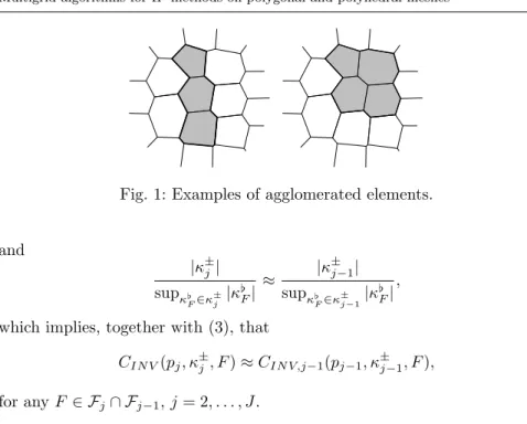
Fig. 1: Examples of agglomerated elements. and |κ±j| supκ♭ F∈κ ± j |κ ♭ F| ≈ |κ ± j−1| supκ♭ F∈κ ± j−1|κ ♭ F| , (21)
which implies, together with (3), that
CIN V(pj, κ±j, F)≈CIN V,j−1(pj−1, κ±j−1, F),
for anyF ∈ Fj∩ Fj−1,j= 2, . . . , J.
Remark 1 The above assumption is satisfied if the agglomeration algorithm preserves the shape-regularity of the elements. In Figure 1, we show two ex-amples of possible macroelements: the agglomerate on the left is not suitable to guarantee assumption (21) due to the presence of a dominant dimension, while the element on the right can be considered appropriate. Moreover, we note that the fulfilment of the above geometric assumptions (20) and (21) can be considered a good criterion in evaluating the quality of the agglomerated grids employed in the multigrid algorithm.
In order to undertake the convergence analysis of the two-level solver out-lined in Algorithm 1, we follow the approach developed in [4]. We then provide an estimate based on the error propagation operator, which is defined as
E2lvlm 1,m2v=G m2 J (IdJ−IJJ−1PJJ−1)G m1 J , (22)
withGJ= IdJ−B−J1AJ, and the operatorPJJ−1:VJ→VJ−1 defined as AJ−1(PJJ−1v, w) =AJ(v, IJJ−1w) ∀v∈VJ, w∈VJ−1. (23) We now study separately thesmoothing propertyand theapproximation prop-erty. Before proceeding with the analysis, we first observe that by Theorem 6, we can boundΛj,j= 1, . . . , J, in (18) as follows
Λj.Ceig(pj) p4 j h2 j .
The last result is employed to prove the smoothing property in the next lemma; see [4, Lemma 4.3] for the proof.
Lemma 6 (Smoothing property) For any v∈Vj,j = 1, . . . , J, we have |||Gmj v|||1,j ≤ |||v|||1,j, |||Gmj v|||s,j .Ceig(pj)(s−t)/2p2(j s−t)h t−s j (1 +m) (t−s)/2|||v||| t,j (24) for0≤t < s≤2andm∈N\ {0}.
Theapproximation propertyresults by exploiting theL2(Ω) error estimates stated in (10) on levelsJ andJ−1.
Lemma 7 (Approximation property) For any v ∈VJ, the following
in-equality holds |||(IdJ−IJJ−1PJJ−1)v|||0,J .CL2(pJ) h2 J−1 p2 J−1 |||v|||2,J. (25)
Proof For anyv∈VJ, we consider the following equality
|||(IdJ−IJJ−1PJJ−1)v|||0,J =k(IdJ−IJJ−1PJJ−1)vkL2(Ω) = sup 06=φ∈L2(Ω) R Ωφ(IdJ−I J J−1P J−1 J )v dx kφkL2(Ω) . (26) Next, we consider the solutionη of the following problem
Z Ω ∇η· ∇v dx= Z Ω φv dx ∀v∈V,
for φ∈ L2(Ω), and let η
J ∈ VJ and ηJ−1 ∈ VJ−1 be the corresponding DG approximations inVJ andVJ−1, respectively, given by
AJ(ηJ, v) = Z Ω φv dx ∀v∈VJ, AJ−1(ηJ−1, v) = Z Ω φv dx ∀v∈VJ−1. (27)
By Theorem 5 and the hypotheses (2) and (3), we deduce that kη−ηJkL2(Ω).CL2(pJ) h2 J−1 p2 J−1 kηkH2(Ω), kη−ηJ−1kL2(Ω).CL2(pJ−1) h2 J−1 p2 J−1 kηkH2(Ω),
and from a standard elliptic regularity assumption, it follows that kη−ηJkL2(Ω).CL2(pJ) h2 J−1 p2 J−1 kφkL2(Ω), kη−ηJ−1kL2(Ω).CL2(pJ−1) h2 J−1 p2 J−1 kφkL2(Ω), (28)
Recalling the definition ofPJJ−1, cf. (23), and (27), for anyw∈VJ−1, we get AJ−1(PJJ−1ηJ, w) =AJ(ηJ, IJJ−1w) =AJ(ηJ, w) = Z Ω φw dx=AJ−1(ηJ−1, w). Hence, ηJ−1=PJJ−1ηJ. (29)
According to [4, Lemma 4.1], the following generalized Cauchy-Schwarz in-equality holds
AJ(v, w)≤ |||v|||0,J|||w|||2,J, (30)
for any v, w ∈ VJ. Next, we observe that by Assumption 2, hypothesis (21)
and (3) we can state the following results for anyF∈ FJ∩ FJ−1
Cm(pJ, F)≈Cm(pJ−1, F), CIN V(pJ, F)≈CIN V(pJ−1, F), Cinterp(pJ)≈Cinterp(pJ−1), G(pJ) ≈ G(pJ−1), which implies that
CL2(pJ)≈CL2(pJ−1).
We now employ (27) and the definition ofPJJ−1 in (23), followed by (29), the Cauchy-Schwarz inequality (30) and the error estimates (28), to get
Z Ω φ(IdJ−IJJ−1PJJ−1)v dx=AJ(ηJ, v)− AJ(ηJ, IJJ−1PJJ−1v) =AJ(ηJ, v)− AJ−1(PJJ−1ηJ, PJJ−1v) =AJ(ηJ, v)− AJ−1(ηJ−1, PJJ−1v) =AJ(ηJ−IJJ−1ηJ−1, v) ≤ |||ηJ−ηJ−1|||0,J|||v|||2,J ≤(kηJ−ηkL2(Ω)+kηJ−1−ηkL2(Ω))|||v|||2,J .(CL2(pJ) +CL2(pJ−1)) h2 J−1 p2 J−1 kφkL2(Ω)|||v|||2,J .CL2(pJ) h2 J−1 p2 J−1 kφkL2(Ω)|||v|||2,J. (31)
Substituting (31) into (26) gives the desired result.
The convergence result for the two-level method, involving the error prop-agation operatorE2lvlm
1,m2 defined in (22), is obtained by combining Lemma 6
and Lemma 7.
Theorem 7 There exists a positive constant C2lvl independent of the mesh
size and the polynomial approximation degree, such that |||E2lvlm
for any v∈VJ, with
ΣJ= ˜C(pJ) p
2
J
(1 +m1)1/2(1 +m2)1/2,
whereC˜(pJ) =Ceig(pJ)CL2(pJ). Therefore, the two-level method converges uni-formly provided the number of pre- and post-smoothing steps satisfy
(1 +m1)1/2(1 +m2)1/2≥χC˜(pJ)p2J,
for a positive constantχ > C2lvl.
Proof The statement of the theorem follows in a straightforward manner by applying the smoothing property (24) twice, the approximation property (25) and exploiting the bounded variation assumptions (2) and (3).
We observe that the rate of convergence is independent of the mesh size, but depends onpJ, as in the case of standard quasi-uniform meshes. Moreover,
a dependence onpJ is also hidden in ˜C(pJ), which also involves the geometric
properties of the partitions. As a consequence, a good quality agglomerated coarse grid is fundamental to guarantee the uniformity of the solver.
4.2 Convergence of the W-cycle multigrid algorithm
As mentioned at the beginning of Section 2, we recall that in the multilevel case, Assumption 1 represents a critical issue. In the following analysis, we then assume that the number of levels is limited, in such a way that the number of interfaces on each level can be bounded by a constant CF that does not
lead to an excessive over-penalization due to the penalization parameterCj σ,
j= 1, . . . , J.
To proceed, we first need to establish the equivalence between DG norms on subsequent grid levels. We point out that, in contrast to the case of standard quasi-uniform grids presented in [4], such an equivalence result does not follow in a straightforward manner; indeed, here we need to exploit the hypotheses (20) and (21) introduced in the previous section. Under these assumptions, the proof of the following result follows immediately.
Lemma 8 Assuming(21)holds, then for anyv∈Vj−1,j= 2, . . . , J, we have
that
kvkDG,j ≤CequivkvkDG,j−1, (33) whereCequiv=Cequiv(Θ), in general, depends on the quality of the agglomerated grids.
Lemma 8 is essential to deduce the stability of the operators Ijj−1 and
Lemma 9 There exists a positive constantCstab, independent of the mesh size, the polynomial approximation degree and the levelj,j = 2, . . . , J, such that
|||Ijj−1v|||1,j ≤Cstab|||v|||1,j−1 ∀v∈Vj−1, (34) |||Pjj−1v|||1,j−1≤Cstab|||v|||1,j ∀v∈Vj. (35)
The proof of Lemma 9 is based on employing inequality (33); for details, see [4, Lemma 4.6].
Remark 2 We stress that the constantCstab depends on Cequiv in (33), which means that the quality of the agglomerated meshes plays a crucial role in keeping this constant bounded, thus resulting in the uniformity with respect to the mesh size and the number of levels as shown in Theorem 8 below.
The error propagation operator associated to Algorithm 2 is defined as
( E1,m 1,m2v = 0 Ej,m 1,m2v =G m2 j (Idj−Ijj−1(Idj−E2j−1,m1,m2)P j−1 j )G m1 j v, j= 2, . . . , J, (36) whereGj= Idj−Bj−1Aj andPjj−1is defined analogously to (23), cf. [21, 13].
Then the convergence estimate for the W-cycle multigrid scheme follows from Theorem 7 and the stability estimates (34) and (35).
Theorem 8 Let C2lvl and Cstab be defined as in Theorem 7 and Lemma 9,
respectively. Then, there exists a constant bC>C2lvl, independent of the mesh size, the polynomial approximation degree and the level j,j = 1, . . . , J, such that, if the number of pre- and post-smoothing steps satisfy
(m1+1)1/2(m2+1)1/2≥ p2jC˜(pj)C 2 stabbC2 b C−C2lvl if ˜ C(pj−1)≤C˜(pj), p2j ˜ C(pj−1)2 ˜ C(pj) C2 stabCb2 b C−C2lvl otherwise, (37) then |||Ej,m 1,m2v|||1,j ≤CbΣj|||v|||1,j ∀v∈Vj, (38) with Σj= ˜C(pj) p2 j (1 +m1)1/2(1 +m2)1/2. (39) Proof The proof follows the derivation of the analogous result presented in [4, Theorem 4.7]. Forj = 1, the statement of the theorem trivially holds. For
j >1, by an induction hypothesis, we assume that (38) holds forj−1. By the definition of the error propagation operatorEj,m
1,m2v in (36), it follows that |||Ej,m 1,m2v|||1,j ≤ |||G m2 j (Idj−Ijj−1P j−1 j )G m1 j v|||1,j +|||Gm2 j I j j−1E2j−1,m1,m2P j−1 j G m1 j v|||1,j.
The first term corresponds to a two-level method between leveljandj−1. We now observe that the smoothing property of Lemma 6 and the approximation property of Lemma 7 can be extended to any levelVj, j = 2, . . . , J, and we
therefore have, by Theorem 7, that |||Gm2 j (Idj−Ijj−1P j−1 j )G m1 j v|||1,j ≤C2lvlΣj|||v|||1,j.
The bound on the second term is obtained by applying the smoothing property (24) forj = 2, . . . , J, the stability estimates (34) and (35) and the induction hypothesis; thereby, we get
|||Gm2 j I j j−1E2j−1,m1,m2P j−1 j Gmj 1v|||1,j ≤C2stabbC2Σj2−1|||v|||1,j. We then obtain |||Ej,m 1,m2v|||1,j ≤ C2lvlΣj+C2 stabCb2Σj2−1 |||v|||1,j.
We now boundΣj−1 withΣj as follows: if ˜C(pj−1)≤C˜(pj), then
Σ2 j−1= ˜C(pj−1)2 p4 j−1 (1 +m1)(1 +m2)≤C˜(pj) 2 p 4 j (1 +m1)(1 +m2) (40) = ˜C(pj) p 2 j (1 +m1)1/2(1 +m2)1/2Σj. Otherwise, Σj2−1= ˜C(pj−1)2 p4 j−1 (1 +m1)(1 +m2) ≤ ˜ C(pj−1)2 ˜ C(pj) p4 j (1 +m1)(1 +m2) (41) ≤C˜(pj−1) 2 ˜ C(pj) p2 j (1 +m1)1/2(1 +m2)1/2Σj. For ˜C(pj−1)≤C˜(pj) by (40), we have that
C2lvlΣj+C2 stabCb 2Σ2 j−1≤ C2lvl+C2stabbC 2C˜(p j) p2 j (1 +m1)1/2(1 +m2)1/2 ! Σj.
We then observe that ifm1 andm2 are such that
(1 +m1)1/2(1 +m2)1/2≥p2 jC˜(pj) C2 stabCb2 b C−C2lvl, it follows that C2lvlΣj+C2 stabCb2Σj2−1≤bCΣj.
For ˜C(pj−1) > C˜(pj), starting from (41) and following the same steps, we deduce the statement of the theorem, providedm1andm2 are such that
(1 +m1)1/2(1 +m2)1/2≥p2j ˜ C(pj−1)2 ˜ C(pj) C2 stabCb2 b C−C2lvl.
As in the two-level case, inequality (38) implies that the convergence of the method is guaranteed if the number of smoothing steps is chosen sufficiently large, cf. (37). Moreover, compared to the case of standard quasi-uniform grids, cf. [4], the bound (37) on the number of smoothing steps involves a strong dependence on the geometrical properties of the underlying agglom-erated meshes, which in principle, could lead to restrictive conditions on the hierarchy of grids employed. However, we remark that, in practice, the nu-merical simulations indicate that the proposed multigrid algorithms converge uniformly, even when low quality agglomerated grids are employed; moreover, an increase in the polynomial order does not seem to require a higher number of smoothing steps to obtain a convergent iteration, cf. Section 5 for details. Remark 3 Whenever the agglomerated grids are not quasi-uniform,i.e., As-sumption 4 is not satisfied, Theorem 7 and Theorem 8 still hold. More precisely, we need to introduce the ratioθjbetween the maximum and minimum element
size on levelj
θj=
maxκ∈Tjhκ
minκ∈Tjhκ
, j= 1, . . . , J.
Moreover, we assume that there exists a constant Cmesh, independent of the granularity of the mesh, such that
θj ≤Cmesh, j= 1, . . . , J.
Then the results in Theorem 7 and Theorem 8 hold with
Σj=θj2C˜(pj)
p2
j
(1 +m1)1/2(1 +m2)1/2, cf. (39), and the bound (37) is modified as follows
(1+m1)1/2(1+m2)1/2≥ C2 stabbC 2 b C−C2lvl C4 mesh θ2 j ˜ C(pj)p2 j if ˜C(pj−1)≤C˜(pj), C2 stabCb2 b C−C2lvl C4 mesh θ2 j ˜ C(pj−1)2 ˜ C(pj) p 2 j otherwise. (42) Remark 4 We recall that in Theorem 8 and Remark 3, in order to guarantee the convergence of the method, we require a lower bound on the number of smoothing steps, cf. (37) and (42). In fact, for ˜C(pj−1)≤C˜(pj), we obtain
b CΣj=Cbθ2jC˜(pj) p 2 j (1 +m1)1/2(1 +m2)1/2 ≤ b C−C2lvl C2 stabCb θ4j C4 mesh ˜ C(pj)p2 j ˜ C(pj)p2 j ≤ Cb−C2lvl C2 stabCb C4 mesh C4 mesh <1.
An analogous result can be obtained for ˜C(pj−1)>C˜(pj). Moreover, we note that we have considered the general case of (42), since (37) can be regarded as a particular case.
Set 1 Set 2 Set 3 Set 4
G1
G2
G3
G4
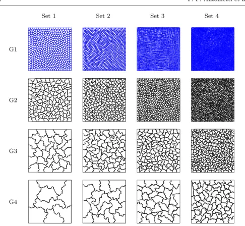
Fig. 2: Sets of nested grids employed for numerical simulations.
5 Numerical results
In this section we present several numerical simulations to verify the theo-retical estimates provided in Theorem 7 and Theorem 8 in the case of a two dimensional problem on the unit squareΩ= (0,1)2. For the numerical tests, we consider the sets of meshes shown in Figure 2. The initial polygonal element meshes are generated using the software packagePolyMesher[35], and consist of 512 (Set 1), 1024 (Set 2), 2048 (Set 3) and 4096 (Set 4) elements. Each ini-tial grid is then subsequently coarsened in order to obtain a sequence of nested partitions by employing the software package MGridGen [26, 27]. Before test-ing the performance of the two-level and W-cycle multigrid solvers presented in Algorithm 1 and Algorithm 2, respectively, we first address the issue of the choice of the penalization coefficient Cj
σ in (4). According to Lemma 2, the
bilinear form Aj(·,·) is coercive provided that Cσj > CF, with CF an upper
bound for the maximum number of element interfaces in the partitionTj; see
Assumption 1. In Table 1, we report the coercivity constantCcoerc of (7) for a fixed value of Cj
σ ≡ Cσ = 10 for j = 1, . . . ,4. We observe that, despite
the increase in the value ofCF from grid G1 to grid G4, the bilinear form is
Set 1 Set 2 Set 3 Set4 G1 0.7385 0.7375 0.7370 0.7364 G2 0.7624 0.7564 0.7559 0.7545 G3 0.7827 0.7818 0.7720 0.7611 G4 0.8153 0.8054 0.8001 0.7827
Table 1: Value of the coercivity constantCcoerc for the sets of grids considered in Figure 2 withCj σ=Cσ = 10,j = 1, . . .,4. 1 2 3 4 5 6 0.6 0.7 0.8 0.9 1 p Two-level W-cycle, 3 levels
Fig. 3: Estimates of C2lvlΣJ and CbΣ3 in (32) and (38), respectively, as a function ofp, andm1=m2=m= 2p2.
in general does not satisfy the theoretical assumption. As a consequence, in the following, we setCj
σ≡Cσ= 10 forj = 1, . . . ,4.
We now consider the grids in Set 1, and numerically evaluate the constant
C2lvlΣJ,J = 2, in Theorem 7 and the constantCbΣ3in Theorem 8, for the h -version of the two solvers, based on selectingm1=m2=m= 3p2, cf. Figure 3. Here, we observe thatC2lvlΣ2andbCΣ3are roughly (asymptotically) constant, as the polynomial degreepincreases; thereby, this implies that ˜C(pJ),J = 2,3, respectively, is approximatelyO(1), aspincreases.
Next, we investigate the performance of the two-level and W-cycle multi-grid schemes in terms of the convergence factor
ρ= exp 1 N ln krNk2 kr0k2 ,
where N denotes the number of iterations required to attain convergence up to a (relative) tolerance of 10−8andr
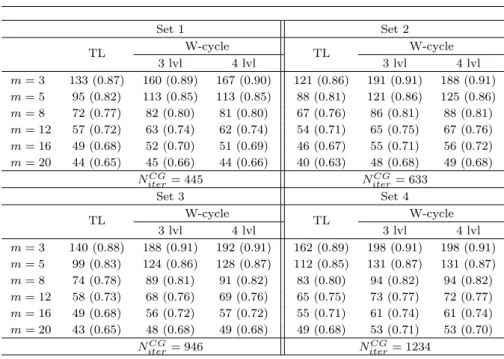
N andr0are the final and initial residual vectors, respectively. In Table 2, we report the iteration counts and the con-vergence factor (in parenthesis), needed to attain concon-vergence of theh-version of the two-level (TL) method and W-cycle multigrid scheme (with 3 and 4 lev-els), as a function of the number of elements (given by the choice of different
Set 1 Set 2 TL W-cycle TL W-cycle 3 lvl 4 lvl 3 lvl 4 lvl m= 3 133 (0.87) 160 (0.89) 167 (0.90) 121 (0.86) 191 (0.91) 188 (0.91) m= 5 95 (0.82) 113 (0.85) 113 (0.85) 88 (0.81) 121 (0.86) 125 (0.86) m= 8 72 (0.77) 82 (0.80) 81 (0.80) 67 (0.76) 86 (0.81) 88 (0.81) m= 12 57 (0.72) 63 (0.74) 62 (0.74) 54 (0.71) 65 (0.75) 67 (0.76) m= 16 49 (0.68) 52 (0.70) 51 (0.69) 46 (0.67) 55 (0.71) 56 (0.72) m= 20 44 (0.65) 45 (0.66) 44 (0.66) 40 (0.63) 48 (0.68) 49 (0.68) NCG iter= 445 NiterCG= 633 Set 3 Set 4 TL W-cycle TL W-cycle 3 lvl 4 lvl 3 lvl 4 lvl m= 3 140 (0.88) 188 (0.91) 192 (0.91) 162 (0.89) 198 (0.91) 198 (0.91) m= 5 99 (0.83) 124 (0.86) 128 (0.87) 112 (0.85) 131 (0.87) 131 (0.87) m= 8 74 (0.78) 89 (0.81) 91 (0.82) 83 (0.80) 94 (0.82) 94 (0.82) m= 12 58 (0.73) 68 (0.76) 69 (0.76) 65 (0.75) 73 (0.77) 72 (0.77) m= 16 49 (0.68) 56 (0.72) 57 (0.72) 55 (0.71) 61 (0.74) 61 (0.74) m= 20 43 (0.65) 48 (0.68) 49 (0.68) 49 (0.68) 53 (0.71) 53 (0.70) NCG iter= 946 NiterCG= 1234
Table 2: Iteration counts and converge factor (in parenthesis) of theh-version of the two-level and W-cycle solvers and iteration counts of the CG method as a function ofm(Cj
σ≡Cσ= 10,p= 1).
Set 1 Set 2 Set 3 TL W-cycle TL W-cycle TL W-cycle
3 lvl 4 lvl 3 lvl 4 lvl 3 lvl 4 lvl m= 3 1281 1334 1342 1168 1272 1362 1230 1379 1391 m= 5 816 832 839 737 790 844 774 852 860 m= 8 546 551 561 487 517 551 513 555 557 m= 12 388 394 400 343 363 385 362 387 384 m= 16 305 312 316 268 284 299 284 301 296 m= 20 254 261 263 222 235 246 235 249 242 NCG
iter= 1954 NiterCG= 2809 NiterCG= 4174
Table 3: Iteration counts of the h-version of the two-level and W-cycle solvers and the CG method as a function of m and the number of levels (Cj
σ ≡Cσ= 10,p= 3).
grid sets), and the number of smoothing steps (m1=m2=m). Here, we have fixed the polynomial approximation order on each level pj ≡p= 1. We first
observe that, although the agglomerated grids, in general, do not necessarily strictly satisfy Assumptions 1 and 2, the number of iterations, for fixed m, does not significantly increase with the number of elements in the underly-ing mesh; moreover, for the W-cycle solver, the number of iterations remains bounded with the number of levels. As expected, the convergence is faster
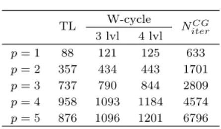
TL W-cycle NCG iter 3 lvl 4 lvl p= 1 88 121 125 633 p= 2 357 434 443 1701 p= 3 737 790 844 2809 p= 4 958 1093 1184 4574 p= 5 876 1096 1201 6796
Table 4: Iteration counts of theh-version of the two-level and W-cycle solvers and the CG method as a function ofpand the number of levels (Cj
σ ≡Cσ= 10,
m= 5).
p= 2 p= 3 p= 4 p= 5
TL TL W-cycle TL W-cycle TL W-cycle 3 lvl 3 lvl 4 lvl 3 lvl 4 lvl m= 12 334 631 1528 860 1028 1051 890 1197 1418 m= 14 292 550 607 748 889 908 772 1033 1220 m= 16 261 489 538 663 784 800 683 910 1071 m= 18 236 441 483 597 703 716 614 814 955 m= 20 216 402 439 543 637 649 558 737 862 NCG iter= 1701 N CG iter= 2809 N CG iter= 4574 N CG iter= 6796 Table 5: Iteration counts of the hp-version of the two-level and W-cycle solvers and the CG method as a function of m and the number of levels (Cj
σ ≡Cσ= 10).
for larger values of m and the solvers are convergent provided the number of smoothing steps is sufficiently large. For each grid, we have also reported the iteration counts NCG
iter for the Conjugate Gradient (CG) method, which
shows that the two proposed solvers outperform the CG scheme in terms of the number of iterations required to attain convergence, even when a small number of smoothing steps are employed. Table 3 presents analogous results for the first three sets of meshes, in the case when p= 3. Here, we observe that, as expected, the convergence factor increases, but the increase inpdoes not require an increase in the minimal number of smoothing steps needed to ensure that the underlying multilevel solvers are convergent.
A more exhaustive investigation of the effect of increasingpis reported in Table 4, where we consider a fine grid of 1024 elements and the corresponding agglomerated meshes (Set 2 in Figure 2). We observe that, even though both multilevel solvers converge for a fixed value ofm, with increasingp, the number of iterations required to attain convergence increases aspgrows. However, the two-level and W-cycle multigrid solvers still employ less iterations, than the number required by the CG method. In Table 5, we report the number of iterations of the hp-version of the two solvers as a function of the number of smoothing steps and the number of levels for varyingp. Here,p=pJ denotes
Triangle Set 1 Triangle Set 2 Triangle Set 3 Triangle Set 4
Fig. 4: Sets of nested grids employed for numerical simulations.
thehp-approach, the polynomial order is decreased from the finest level to the coarser ones in such a way thatpj−1=pj−1. We observe that the introduction
of thehp-multigrid is detrimental for the convergence of the method, since the minimum number of smoothing steps needed to obtain a convergent method increases with respect to the h-version. Then, we can conclude that, as the
p-version of the method does not exhibit uniform convergence with respect to the polynomial order, the hp-approach turns out to be not very effective for problems resulting from high-order discretizations.
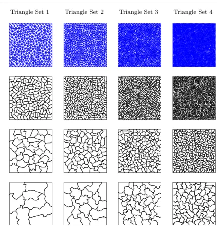
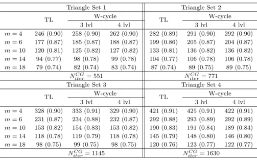
As a second numerical test, we consider the same problem discretized by the interior penalty DG method of Section 2 on an initial mesh of triangles, thus reproducing a more common scenario in the framework of finite element discretizations. In analogy to the case of polygonal meshes, we consider four sets of nested grids obtained by agglomeration, cf. Figure 4. The sets con-sidered derive from initial meshes of 528 (Triangle Set 1), 1086 (Triangle Set 2), 2198 (Triangle Set 3) and 4318 (Triangle Set 4) elements. In Table 6, we show the iteration counts needed to attain convergence with respect to a fixed tolerance of 10−8 as a function of the set (i.e., the number of elements) and the number of smoothing steps of the h-version of the two-level and W-cycle
multigrid solvers, withpj =p= 1. We recall that, as in the previous numerical
test, we have consideredCj
σ ≡Cσ = 10, for eachj. The results are similar to
the case of initial polygonal meshes, with uniform convergence with respect to the granularity of the mesh, and in the case of the W-cycle solver, also with respect to the number of levels. We again attain improved performance, compared to the standard CG method, in terms of the number of iterations required to attain convergence.
Triangle Set 1 Triangle Set 2 TL W-cycle TL W-cycle 3 lvl 4 lvl 3 lvl 4 lvl m= 4 246 (0.90) 258 (0.90) 262 (0.90) 282 (0.89) 291 (0.90) 292 (0.90) m= 6 177 (0.87) 185 (0.87) 188 (0.87) 199 (0.86) 205 (0.87) 204 (0.87) m= 10 120 (0.81) 125 (0.82) 127 (0.82) 133 (0.81) 136 (0.82) 136 (0.82) m= 14 94 (0.77) 98 (0.78) 99 (0.78) 104 (0.77) 106 (0.78) 106 (0.78) m= 18 79 (0.74) 82 (0.74) 83 (0.74) 87 (0.74) 89 (0.75) 89 (0.75) NCG iter= 551 NiterCG= 771
Triangle Set 3 Triangle Set 4 TL W-cycle TL W-cycle 3 lvl 4 lvl 3 lvl 4 lvl m= 4 328 (0.90) 333 (0.91) 329 (0.90) 421 (0.91) 425 (0.91) 422 (0.91) m= 6 231 (0.87) 234 (0.88) 232 (0.87) 292 (0.88) 293 (0.89) 292 (0.89) m= 10 153 (0.82) 154 (0.83) 153 (0.82) 190 (0.83) 191 (0.84) 189 (0.84) m= 14 118 (0.78) 119 (0.79) 118 (0.78) 145 (0.79) 148 (0.80) 146 (0.80) m= 18 98 (0.75) 99 (0.75) 98 (0.75) 120 (0.76) 123 (0.77) 122 (0.77) NCG iter= 1145 NiterCG= 1630
Table 6: Iteration counts and converge factor (in parenthesis) of theh-version of the two-level and W-cycle solvers and iteration counts of the CG method as a function ofm(Cj
σ≡Cσ= 10,p= 1). Starting mesh of triangles.
References
1. Antonietti, P.F., Giani, S., Houston, P.:hp–Version composite discontinuous Galerkin methods for elliptic problems on complicated domains. SIAM J. Sci. Comput.35(3), A1417–A1439 (2013)
2. Antonietti, P.F., Giani, S., Houston, P.: Domain decomposition preconditioners for Dis-continuous Galerkin methods for elliptic problems on complicated domains. J. Sci. Comput.60(1), 203–227 (2014)
3. Antonietti, P.F., Houston, P.: A class of domain decomposition preconditioners forhp -discontinuous Galerkin finite element methods. J. Sci. Comput.46(1), 124–149 (2011) 4. Antonietti, P.F., Sarti, M., Verani, M.: Multigrid algorithms for hp-Discontinuous
Galerkin discretizations of elliptic problems. SIAM J. Numer. Anal. To appear. 5. Arnold, D.N.: An interior penalty finite element method with discontinuous elements.
SIAM J. Numer. Anal.19(4), 742–760 (1982)
6. Arnold, D.N., Brezzi, F., Cockburn, B., Marini, L.D.: Unified analysis of discontinu-ous Galerkin methods for elliptic problems. SIAM J. Numer. Anal.39(5), 1749–1779
7. Aubin, J.: Approximation des probl`emes aux limites non homog`enes pour des op´erateurs non lin´eaires. J. Math. Anal. Appl.30, 510–521 (1970)
8. Babuˇska, I.: The finite element method with penalty. Math. Comp.27(122), 221–228
(1973)
9. Baker, G.A.: Finite element methods for elliptic equations using nonconforming ele-ments. Math. Comp.31(137), 45–59 (1977)
10. Bassi, F., Botti, L., Colombo, A., Brezzi, F., Manzini, G.: Agglomeration-based physical frame dg discretizations: An attempt to be mesh free. Math. Models Methods Appl. Sci.24(8), 1495–1539 (2014)
11. Bassi, F., Botti, L., Colombo, A., Di Pietro, D.A., Tesini, P.: On the flexibility of agglomeration based physical space discontinuous Galerkin discretizations. J. Comput. Phys.231(1), 45–65 (2012)
12. Bassi, F., Botti, L., Colombo, A., Rebay, S.: Agglomeration based discontinuous Galerkin discretization of the Euler and Navier-Stokes equations. Comput. & Fluids
61, 77–85 (2012)
13. Bramble, J.: Multigrid Methods. No. 294 in Pitman Research Notes in Mathematics Series. Longman Scientific & Technical, Harlow, UK (1993)
14. Cangiani, A., Georgoulis, E.H., Houston, P.: hp-Version discontinuous Galerkin methods on polygonal and polyhedral meshes. Math. Models Methods Appl. Sci.24(10), 2009– 2041 (2014)
15. Chan, T.F., Xu, J., Zikatanov, L.: An agglomeration multigrid method for unstructured grids. In: Domain decomposition methods, 10 (Boulder, CO, 1997),Contemp. Math., vol. 218, pp. 67–81. Amer. Math. Soc., Providence, RI (1998)
16. Cockburn, B., Karniadakis, G.E., Shu, C.W. (eds.): Discontinuous Galerkin methods, Springer-Verlag. Berlin (2000). Theory, computation and applications. Papers from the 1st International Symposium held in Newport, RI, May 24-26, 1999
17. Beir˜ao Da Veiga, L., Brezzi, F., Cangiani, A., Manzini, G., Marini, L.D., Russo, A.: Basic principles of virtual element methods. Mathematical Models and Methods in Applied Sciences23(01), 199–214 (2013)
18. Di Pietro, D.A., Ern, A.: Mathematical aspects of discontinuous Galerkin meth-ods, Math´ematiques & Applications (Berlin) [Mathematics & Applications], vol. 69. Springer, Heidelberg (2012)
19. Fries, T.P., Belytschko, T.: The extended/generalized finite element method: An overview of the method and its applications. International Journal for Numerical Meth-ods in Engineering84(3), 253–304 (2010)
20. Georgoulis, E.H.: Inverse-type estimates onhp-finite element spaces and applications. Math. Comp.77(261), 201–219 (electronic) (2008)
21. Hackbusch, W.: Multi-grid methods and applications,Springer series in computational mathematics, vol. 4. Springer, Berlin (1985)
22. Hackbusch, W., Sauter, S.: Composite finite elements for problems containing small geometric details. Part II: Implementation and numerical results. Comput. Visual Sci.
1(4), 15–25 (1997)
23. Hackbusch, W., Sauter, S.: Composite finite elements for the approximation of PDEs on domains with complicated micro-structures. Numer. Math.75(4), 447–472 (1997) 24. Hesthaven, J.S., Warburton, T.: Nodal Discontinuous Galerkin Methods: Algorithms,
Analysis, and Applications, 1st edn. Springer Publishing Company, Incorporated (2007) 25. Lions, J.L.: Probl`emes aux limites non homog`enes `a don´ees irr´eguli`eres: Une m´ethode d’approximation. In: Numerical Analysis of Partial Differential Equations (C.I.M.E. 2 Ciclo, Ispra, 1967), Edizioni Cremonese, Rome, pp. 283–292 (1968)
26. Moulitsas, I., Karypis, G.: Mgridgen/Parmgridgen Serial/Parallel Library for Gen-erating Coarse Grids for Multigrid Methods. University of Minnesota, Depart-ment of Computer Science/Army HPC Research Center (2001). Available at:
www-users.cs.umn.edu/~moulitsa/software.html
27. Moulitsas, I., Karypis, G.: Multilevel algorithms for generating coarse grids for multigrid methods,. In: Supercomputing 2001 Conference Proceedings (2001)
28. Nitsche, J.: ¨Uber ein Variationsprinzip zur L¨osung von Dirichlet Problemen bei Ver-wendung von Teilr¨aumen, die keinen Randbedingungen unterworfen sind. Abh. Math. Sem. Uni. Hamburg36, 9–15 (1971)
29. Reed, W., Hill, T.: Triangular mesh methods for the neutron transport equation. Tech. Rep. LA-UR-73-479, Los Alamos Scientific Laboratory (1973)
30. Rivi`ere, B.: Discontinuous Galerkin methods for solving elliptic and parabolic equa-tions, Frontiers in Applied Mathematics, vol. 35. Society for Industrial and Applied Mathematics (SIAM), Philadelphia, PA (2008). Theory and implementation
31. Schwab, C.:p- andhp-finite element methods. Numerical Mathematics and Scientific Computation. The Clarendon Press, Oxford University Press, New York (1998). Theory and applications in solid and fluid mechanics
32. Stein, E.: Singular Integrals and Differentiability Properties of Functions. Princeton, University Press, Princeton, N.J. (1970)
33. Sukumar, N., Tabarraei, A.: Conforming polygonal finite elements. International Journal for Numerical Methods in Engineering61(12), 2045–2066 (2004)
34. Tabarraei, A., Sukumar, N.: Extended finite element method on polygonal and quadtree meshes. Computer Methods in Applied Mechanics and Engineering 197(5), 425–438
(2008)
35. Talischi, C., Paulino, G., Pereira, A., Menezes, I.: Polymesher: A general-purpose mesh generator for polygonal elements written in matlab. Structural and Multidisciplinary Optimization45(3), 309–328 (2012)
36. Wheeler, M.F.: An elliptic collocation-finite element method with interior penalties. SIAM J. Numer. Anal.15(1), 152–161 (1978)