Pork Barrel Cycles ∗

Pork Barrel Cycles

∗

Allan Drazen

_{Marcela Eslava}

This Draft: April 2006

Abstract

We present a model of political budget cycles in which incumbents influence voters by targeting government spending to specific groups of voters at the expense of other voters or other expen-ditures. Each voter faces a signal extraction problem: being targeted with expenditure before the election may reflect opportunistic manipulation, but may also reflect a sincere preference of the incumbent for the types of spending that voter prefers. We show the existence of a political equilibrium in which rational voters support an incumbent who targets them with spending before the election even though they know it may be electorally motivated. In equilibrium voters in the more “swing” regions are targeted at the expense of types of spending not favored by these voters. This will be true even if they know they live in swing regions. However, the responsiveness of these voters to electoral manipulation depends on whether they face some degree of uncertainty about the electoral importance of the group they are in. Use of targeted spending also implies voters can be influenced without election-year deficits, consistent with recent findings for established democracies.

JEL classification: D72, E62, D78

Keywords: expenditure composition, political budget cycle, special interest groups, electoral manipulation

∗_{We wish to thank seminar participants at IIES-Stockholm University, the NBER Working Group Meeting on} Polit-ical Economy, Tel Aviv University, the LACEA PolitPolit-ical Economy Network, and Yale University for useful comments. We also thank Miguel Rueda for excellent research assistance. Drazen’s research was supported by the National Science Foundation, grant SES-0418482, the Israel Science Foundation, and the Yael Chair in Comparative Economics, Tel-Aviv University.

†_{Jack and Lisa Yael Professor of Comparative Economics, Tel Aviv University, University of Maryland, NBER, and} CEPR. Email: drazen@econ.umd.edu

1

Introduction

Conventional wisdom is that incumbents use economic policy — especially fiscal policy — before elections to influence electoral outcomes. A number of studies (Shi and Svensson [2006], Persson and Tabellini [2003]) find evidence of an electoral deficit or expenditure cycle in a broad cross-section of countries, an empirical finding that Brender and Drazen (2005a) argue reflects electoral cycles in a subset of these countries, namely those that recently democratized. These “new democracies” are characterized by increases in government deficits in election years in the first few elections after the transition to democracy. In contrast, in “established” democracies, they find no statistically significant political cycle across countries in aggregate central government expenditure or deficits, a finding which is robust to various specifications.

The finding of no political deficit cycle in established democracies raises an obvious question: Is fiscal manipulation absent or, more likely, does it simply appear in different forms? That is, in established democracies, do politicians use election-year fiscal policy to influence voters in such a way that the overall government budget deficit is not significantly affected? This could occur, for example, if some groups of voters are targeted at the expense of others. Groups whose voting behavior is seen as especially susceptible to targeted fiscal policy may be targeted with higher expenditures and transfers, or by tax cuts, financed by expenditure cuts or tax increases on other groups whose votes are much less sensitive to such policy. Such election-year “pork barrel spending”, by which we mean policies or legislation targeted to specific groups of voters to gain their political support, is widely seen as an especially important component of electoral manipulation. Policies of this type include geographically concentrated investment projects (a common, more narrow definition of “pork barrel spending”), expenditures and transfers targeted to specific demographic groups, or tax cuts benefitting certain sectors.1 In this paper, we develop a model of electoral manipulation via targeting specific groups of voters with government spending, where there is no effect on total spending or the deficit.

Several papers find evidence of significant changes in the composition of government spending in election years. Khemani (2004) finds that Indian states spend more on public investment before scheduled elections that in other times, while they contract current spending, leaving the overall balance unchanged. Kneebone and McKenzie (2001) look for evidence of a political budget cycle

1

An alternative possibility is a change in the composition of expenditures towards those that are highly valued by voters as awhole and away from those that are less valued. If politicians are believed to differ in their (not directly observed) preferences over types of expenditures, all voters will prefer a politician whose preferences are more towards expenditures that they prefer. We study such a set-up in Drazen and Eslava (2005).

for Canadian provinces, and find no evidence of a cycle in aggregate spending, but dofind electoral increases in what they call “visible expenditures”, mostly investment expenses such as construction of roads and structures. Very similarfindings are reported for Mexico by Gonzales (2002), who alsofinds that other categories of spending, such as current transfers, contract prior to elections. Drazen and Eslava (2005) present empirical evidence on compositional effects in regional political budget cycles in Colombia, where investment projects grow before elections, while current spending contracts. Interestingly, electoral composition effects seem to imply expansions in development projects, which are in general easily targeted. Khemani (2004), for instance, argues that hisfinding of greater public investment before elections suggests that election-year policy takes the form of targeting of special interests, rather than an attempt to sway the mass of voters at large.

The evidence of electoral effects on the composition of spending, rather than on the overall deficit, is consistent withfindings on how voters react to election-year government deficits, both in individual country and in cross-section studies. Brender (2003) finds that voters in Israel penalize election year deficits, but also that they reward high expenditure in development projects in the year that precedes an election. Similarly, Peltzman’s (1992) result that U.S. voters punish government spending holds for current (as opposed to capital) expenditures, but is weaker if investment in roads, an important component of public investment, is included in his policy variable. Drazen and Eslava (2005)find that voters in Colombia reward high pre-election public investment, but only to the extent that this extra spending is not obtained at the expense of larger deficits. Alesina, Perotti, and Tavares (1998) look at election outcomes and opinion polls for 19 OECD countries andfind that after sharpfiscal adjustments based mostly on current spending cuts, the probability that an incumbent remains in power does not fall. Perhaps the strongest evidence suggesting that deficits do not help reelection prospects comes from Brender and Drazen (2005b) in a sample of 74 countries over the period 1960-2003. They find no evidence that deficits help reelection in any group of countries, including developed and less developed, new and old democracies, countries with different government or electoral systems, and countries with different levels of democracy. In developed countries and established democracies, they find that election-year deficits actually significantlyreduce the probability that a leader is reelected. In short, the strategy of using targeted increases in spending before elections financed by cuts on some other types of spending rather than by increased deficits seems to be optimal for an incumbent seeking re-election.

In spite of the widespread use of policies targeted at specific groups of voters or types of expen-ditures before elections, there are no rational-voter models of the political cycle integrating targeted

expenditures that are truly intertemporal. Lindbeck and Weibull (1987) and Dixit and Londregan (1996) present formal models where, in order to gain votes, candidates make promises of spending to some voter groups (based on their characteristics) financed by cuts in spending on other groups so as to keep the government budget balanced. However, they assume that campaign promises are binding commitments to a post-electoral fiscal policy. Hence, in these models the problem of who gets targeted is essentially a static one, with no voter inference problem about post-electoral utility based on the pre-electoral economic magnitudes announced by candidates.2 Hence, these models do not really answer a key question: Why would rational, forward-looking voters who are targeted by the incumbent before the election find it optimal to vote for him? The answer is far from obvious: if Floridians know that politicians target them solely because of a forthcoming election, why would they believe that such spending will continue after the incumbent is reelected? This paper squarely addresses this question, incorporating expenditure targeting in a framework of repeated elections with rational voters.3

The best known approach in modeling why rational, forward-looking voters might respond to election-year economics was introduced by Rogoff and Sibert (1988) and Rogoff (1990), based on the unobservability of an incumbent’s ability or “competence” in providing aggregate expenditures without raising taxes.4 More “competent” candidates can provide more public goods at a given level of taxes, and hence generate higher welfare, so they are preferred by voters. Since competence is correlated over time, a candidate who is inferred by voters to be more competent than average before the election is expected to be so after the election as well.5 Voters rationally prefer a candidate from whom they observe higher expenditures before an election, since this is a signal of higher competence, implying higher overall expenditure after the election.

A key ingredient of various models focussing on competence is voters’ inability to observe the overall level of spending or of the deficit (Rogoff [1990], Shi and Svensson [2006]). Because of this assumption, the competence approach often implies an increase in total government expenditures (or

2

Most other papers that consider the allocation of “pork” across different groups of voters (Myerson (1993), Persson, Roland, and Tabellini (2000), Lizzeri and Persico (2001)) similarly assume that candidates make binding promises to voters. Grossman and Helpman (2005) do not assume binding promises. However, as in the other papers, pre-electoral distribution of porkper seplays no role in determining election outcomes. Furthermore, in their paper there is no voter uncertainty about policymakers preferences over the allocation of pork, which is central to our approach.

3

Strömberg (2005) presents an interesting model of the campaign visits by presidential candidates to different U.S. states (a type of targeting), but where voter response to targeting is assumed rather than derived from primitives.

4

Other rational voter models include Persson and Tabellini (1990), González (2001), Stein and Streb (2004), and Shi and Svensson (2006). All of these models share with the Rogoffapproach a reliance on the effect of pre-electoral fiscal expansion on expected aggregate activity or welfare after the election.

5

A key innovation of Shi and Svensson (2006) is that the policymaker chooses fiscal policy before he knows his competence level, so that all “types” choose the same level of expansion. That is, the model focusses on moral hazard rather than signaling, as do the other models. An implication is an aggregate deficit cycle.

in the government budget deficit) in an election year. This relation between voters’ lack of information and aggregate fiscal expansion is consistent with Brender and Drazen’s (2005a) empirical finding of no statistically significant aggregate deficit or expenditure cycle in established democracies, where voters may be well informed about fiscal outcomes.

The absence of political budget cycles in democracies where voters are experienced and presumably informed about fiscal policy (and the further finding of Brender and Drazen [2005b] that higher election-year expenditures or deficits do not increase an incumbent’s probability of reelection in these democracies), suggests that rational voters may be trying to infer something other than (or in addition to) competence from election-yearfiscal policy. That is, these empiricalfindings suggest that imperfect information about competence alone is not a sufficient basis for an asymmetric information explanation of voter response to election-year policies. On the other hand, since expenditure targeted at some groups of voters is a common form of election-year policy, voters may use pre-election economic policy to learn not primarily the likely level of post-electoral expenditure (if the incumbent is re-elected) as in the competence approach, but the composition of expenditure across groups of voters. Put simply, voters targeted before an election want to know whether they will be similarly favored after the election if the incumbent is re-elected.

If voters are indeed using pre-election spending to make inferences about the composition of government spending after the election, one wonders: What makes it credible that a politician will continue to favor the same groups after the election that he targeted before? Our argument is that politicians have unobserved preferences over groups of voters or types of expenditure, preferences that have some persistence over time. This persistence implies that a voter who believes that the incumbent favors him before the election rationally expects some similarity in the composition of expenditures after the election as well.6

This change from the competence approach in the unobserved characteristic of incumbents sig-nificantly changes the nature of the inference problem that voters face. In models in the Rogoff

tradition, a voter must infer whether high pre-electoral expenditure on an observable component of the budget reflects higher incumbent ability to provide goods in general, or whether it is “purchased” at the expense of a cut in some other good (or a tax increase) observed only after the election. In our model, instead, a voter knows how a change in spending was financed and what was the total spending, but tries to learn to what extent the pre-election composition of spending will be replicated

6_{Another argument is that politicians who renege on the (implicit) commitment to continue a government program}

after the election may lose the ability to usefiscal policy as a tool to influence voters in future elections. This may make the pre-election composition of expenditure a credible signal of the composition the incumbent would choose if re-elected.

after the election and, based on that inference, whether he will be better offunder the incumbent or the challenger. As a result, electoral fiscal policy may be present even if voters can perfectly observe all of the elements of fiscal policy. This is one key difference between our model and those in the competence tradition.

In our approach, moreover, a voter may have imperfect information both about the politicians’s preferences over different voter groups and about voting patterns over the population. If both types of asymmetric information are present, each voter must try to infer whether receiving high targeted expenditures before the election signals a high weight of his group in the incumbent’s objective func-tion (relative to other voters or to non-targeted expenditures) or simply how “swing” his demographic group is, meaning how many votes the incumbent can raise by targeting his group with expenditures. Put more simply, a politicians tries to convince a voter that he truly “likes” him (or has the same objectives), while voters wonder whether the expressions of love and caring will disappear once the votes are counted.

Our emphasis on cycles in the composition of spending, rather than its overall level, is consistent with the evidence cited above that voters are “fiscal conservatives” who punish (rather than reward) high spending or deficits at the polls. Our model in fact suggests that, if voters are averse to deficits, observability of fiscal policy strengthens the incentive to finance electoral spending through the contraction of other expenditures. The greater ability of voters to monitor fiscal outcomes in established democracies may help explain the absence of significant political deficit cycles.

Another key difference with the competence literature is that political budget cycles in our model arise even if all politicians are equally able to provide public goods. We assume here that all politicians are equally competent in delivering pork in order to obtain a clear contrast with that literature, rather than because we think competence is unimportant. We are aware that in a system with geographically defined districts, legislators often campaign for reelection on the basis of their ability to obtain projects for their district. However, if competence in getting pork is general and not specific to a demographic group (as, for example, Dixit and Londregan [1996]) or type of expenditure (as in Strömberg [2001]), demonstrating competence in delivering pork may be necessary to be reelected, but it would not be sufficient. Suppose a specific group of voters believed that a politician was very competent in delivering pork, but also believed that he did not care about them at times other than elections. These voters would then expect that after the election he will use his pork-raising competence to benefit other groups, so they would have no reason to vote for him on the basis of high perceived

competence.7 Hence, preferences over groups of voters seem crucial in explaining pork-barrel politics. In reality, both politician competence and politician preferences are no doubt important in explaining the importance of pork in elections, but here we focus on the role of the latter, which has not been much explored.

In a model with asymmetric information about the preferences of politicians, and possibly also with asymmetric information about how “swing” different groups in society are, we demonstrate that there exists a Perfect Bayesian Equilibrium in which voters rationally respond to election-year expen-ditures and politicians allocate expenditure across groups on the basis of this behavior. Politicians increase spending targeted to electorally attractive groups before elections, while they contract other types of expenditure to satisfy the no-deficit constraint. As mentioned, a key result is that electoral manipulation arises even with fully rational voters. We further show that the responsiveness of voters tofiscal manipulation depends on the amount of information they have about how “swing” different groups are; however, a political cycle arises even when voters know how “swing” each group is.

The plan of the paper is as follows. In the next section we present an overview of our approach. In section 3 we present a model of politicians with unobserved preferences over groups of voters. In section 4 we show the existence of a Perfect Bayesian Equilibrium for this model with rational, forward-looking voters in which there is a political cycle in the composition of expenditure. In section 5 we add a good valued only by politicians (“office rents”) to show that electoral fiscal manipulation might entail some groups being targeted at the expense of others, or all voter groups being targeted at the expense of office rents that politicians value. Because of the difficulty of analyticallyfinding an equilibrium, in section 6 we present an example which illustrates the political equilibrium. Conclusions are presented in section 7.

2

An Overview

To help readers better understand the detailed model in section 3, wefirst present an outline of our basic argument. We exposit the model in terms of geographically-targeted expenditure, which is important in many political systems, but stress that our argument applies equally well to spending that can be targeted at groups defined along dimensions other than the geographical. Hence, our analysis is relevant not only to majoritarian systems with geographically defined districts, but also to other types of electoral systems, such as proportional systems, in which parties may target different

7_{This issue does not arise in the Rogoff(1990) model since competence is used to provide public goods that benefit}

types of voters. (This is consistent with our broad definition of “pork barrel spending” set out in the introduction.)

Furthermore, though policy is made by a single policymaker, as in a stylized presidential system, the basic argument is applicable to parliamentary systems in which policy is the result of bargaining within a legislature. In such models, bargaining strength in the legislature depends on vote shares, but the nature of legislative interactions means that policy outcomes may depend in complicated ways on the vote share that a party receives. Sophisticated voters with policy preferences may thusfind it optimal to vote strategically rather than sincerely in a multi-candidate election, as in the models of Austen-Smith and Banks (1988) or Baron and Diermeier (2001). However, since parties attract votes on the basis of the policy preferences voters perceive that they have, the key voter inference problem in our model should be crucial in parliamentary systems as well. In short, though we exposit our model in a way consistent with a specific set of electoral and legislative rules, we believe that the analysis is applicable to a far broader set of political institutions.

We assume that there is an election between an incumbent and a challenger at the end of every other period (“year”)t, t+ 2, etc. The incumbent has the ability to choose fiscal policy, where, for simplicity, we focus on the targeting of expenditures, and simply assume (in line with voters being fiscal conservatives) that incumbents can neither raise taxes, nor incur deficits. Hence, the sum of all expenditures must always equal the fixed level of taxes.

There are two regions, h = 1,2, where voters in each region value a public good gh_t supplied to their region. Since taxes are assumedfixed, we abstract here from other types of consumption which could be affected by tax policy. The utility of individualj in region h also depends on the distance between his most desired positionπj _{over other policies (which is immutable and termed “ideology”)}

and the positionπP of the politicianP in power.

Within each regionh, there is a non-degenerate distribution of ideological preferences, which may change between elections. We denote the density function of voters in regionhin the current election cycle as fh(π), where we suppress the time subscript. We consider both the case where the fh(π)

are known to both voters and politicians, as well as the case of asymmetric information where the incumbent knows the densitiesfh(π), while voters only have imperfect information about them. The

nature of the cycle is affected by the information specification, but in both cases a rational political cycle exists. For simplicity, we assume that the preference distribution is uncorrelated over elections, so that past electoral policy gives voters no information about the current distribution.

πR as given and assume no competition over ideology. Without loss of generality, we assume that party Lis the incumbent.

The single-period utility of a voter in region h with ideological preferences πj if policymaker A_∈{L, R_} is in office is

U_sh, j(A) = lng_sh(A)₋¡πj₋πA¢2 (1) where gh_s(A) is public good provided by policymaker A to region h in period s. Voters care about the present discounted value of utility, and hence, about expected future values ofg_sh. (Sincegh_s(A)

does not depend on j, we ignore the index j in discussing the central problem of inferringg_th₊₁ from gh_t.)

Politicians, as actual or potential leaders of both regions, give weight to the utility from govern-ment spending of voters of each region.8 This may be represented by a weight ωh_P,s that politician P puts on utility from public goods of residents of that region, that is, on lng_th. (Since ideological preferences πj of both voters and politician’s are fixed, putting the weight ωh_P,s on a voter’s total utility (1) would not qualitatively change the basic results.) A politicianP’s single-period utility in periodsif the policy in place is πAmay be written

U_sP =Z_sP(gs)−

¡

πP ₋πA¢2 (2)

wheregs is the vector

¡ g1_s, g2_s¢and Z_sP(gs) = 2 X h=1 ωh_P,slng_sh . (3)

In contrast to the politician’s ideological preferences πP which are known, the weights ωh_P,s are unknown to voters.9 The key inference problem giving rise to the possible effectiveness of election-year spending in influencing rational voters may now be stated. The voter’s problem is to infer the unobserved weightωh_P,tfrom the politician’s observable choice ofgh_t. Ifωh_P,thas some persistence over

8

The difference between the objective functions of politicians and voters consistent with the “citizen-candidate” approach of Besley and Coate (1997) or Osborne and Slivinski (1996). A key message of that approach is that because candidates have preferences just like citizens, they can be expected to act on those preferences once elected, rather than be bound by campaign “promises”. This view is in fact central to our approach, where a voter’s key inference problem is in discerning what those preferences are. We diverge from the basic citizen-candidate model in assuming that a citizen who is elected to make policy for an area wider than his or her own district will no longer act on the same (narrower) preferences he or she did when being a simply a member of (or representing) that district. We would argue that this assumption is quite reasonable. We do not model this “transformation” of preferences.

9_{Bonomo and Terra (2005) consider politicians who have preferences over sectors, but where these preferences are}

time, then pre-electoral g_th may contain information not only aboutωh_P,t, but also about ωh_P,t+1 and henceg_th₊₁, inducing forward-looking voters to respond to pre-electoralfiscal policy.10

Why would voters not know a politician’s preferences? (See footnote 8 on why these preferences are not identical to those of a citizen from the politician’s region.) That is, there really an inference problem? We would argue that since the real world is multidimensional, a voter is necessarily uncer-tain about how much the politician will favor him relative to other priorities. Moreover, because the politician’s environment changes over time, these preferences may change over time, but at the same time will display some persistence.

Another key question is why voters look atfiscal policy only right before the elections, in order to try to infer a politician’s preferences, rather than at policy earlier in the incumbent’s term. As in most of the literature, we assume that unobserved preferences (here ωh_P,t) are evolving over time in such a way that the most recent policy observation is the more informative about future policy than earlier observations.11 We believe this partly captures the evolution of a politician’s preferences, which may change over time (albeit slowly), justifying voters’ concentration on recent policy to infer these preferences. The media follow policy more as elections get closer, reflecting greater voter interest in policy developments closer to elections. This suggests perhaps that voters believe that they have more to learn closer to elections, but may also be a reason why voters are more responsive to pre-election policy.

We now turn to the details. We start by looking at the problem of an incumbent politician, given the fiscal framework, then move to the voters’s problem, andfinally put the pieces together to find the equilibrium.

3

A Model of Politicians Who Have Preferences over Voters

3.1

The Incumbent’s Problem

Politicians differ in the unobserved weightωh_P,sthey put on voters of the two regions (or groups) in their objective function (2), as summarized by (3). For simplicity, we assume that ωh_P,s is drawn from an i.i.d. distribution at the beginning of every election year for two years and thatω2_P,s= 1₋ω1_P,s. (That is,ωh_P,t+1=ωh_P,t iftis an election year, but ωh_P,t and ωh_P,t+2 are uncorrelated.) No correlation

1 0

In the case where voters in the two regions care about both goods, targeting would be of a good rather than of a region (which in this formulation are identical.) See footnote 17.

1 1

In contrast to the standard approach in the literature, Martinez (2005) presents a very different type of model of how an incumbent’s performance reputation might evolve over time and shows that policy outcomes closest to the elections may not necessarily provide the most information about unobserved politician characteristics.

inωh_P,s across electoral cycles greatly simplifies the voters’s inference problem, since observed policy in previous elections provides no information about current ωh_P,s.12 The distribution of ωh_P,t, which is the same for both incumbent and challenger, is defined over¡ωl, ωu¢, where 0_≤ωl< ωu _≤1 and has a mean ofω.

3.1.1 The off-year decision

A politician Lwho was elected inthas an objective functionΩIN_t+1 in the following non-election year t+1(when he isin office and not facing an election int+1) for the vector of public goods expenditure

g_tL₊₁ of ΩIN_t+1(gL_t+1, L) = 2 X h=1 ωh_P,t+1lng_th₊₁+βE_tL₊₁¡ΩELE_t+2 (_·, L)¢ (4)

where β is the discount factor andE_tL₊₁¡ΩELE_t+2 ¢is L’s expectation as of period t+ 1 of the present discounted value of utility from t+ 2 (an election year) onward. (Since the actual policy πA _=πP_,

(2) and (3) yield current-period utility ofP_hωh_P,slngh_s in an off-election year.) The assumptions that the government’s budget is balanced each period and thatωh

Las ofthas a two-period life imply that

actions at t+ 1 have no effect on ΩE_t+2. The incumbent’s off-year problem is simply to choose the gh_t+1 to maximizeP2_h=1ωh_P,t+1lng_th₊₁ subject to his budget constraint.

Total expenditures equal total tax revenues, which are assumed fixed and set equal to unity. (All politicians are thus identical in terms of total spending.) The choice offiscal policy is the choice of composition of the government budget, which comprises expenditures that can be targeted to specific groups of voters, and other types of expenditure. For simplicity, in this section, we assume that there are no expenditures other than public goods g1 and g2. (In section 5 we consider the implications of politicians also spending on goods that they alone value, that is, “office rents”.) Therefore, each period, the government faces the budget constraint:

g_s1+g_s2= 1 s=t, t+ 1, . . . (5)

The first-order condition for the politician’s off-election year problem is:

1 2

AssumingωhP,s follows an MA(1) process with innovations that are revealed to voters with a one-period lag has

these implications. This alternative type of assumption is, for instance, the one used in Rogoff (1990). A political budget cycle would also arise with an MA(1) process with innovations that are never revealed to voters, as long as imperfect persistence ofωh

P,smakesgth−1 a more relevant signal to voters than expenses observed further into the past.

ω1_L g1 t+1 = ω 2 L g2 t+1 (6) where, for ease of exposition, we drop the time subscript onωh_L,s, that is, we writeωh_L,t=ωh_L,t+1=ωh_L. Usingω2_L= 1₋ω1_L and g_t2₊₁= 1₋g1_t+1 from (5),

g_th₊₁ =ωh_L h= 1,2 (7)

so that voters’s expected utility from reelecting the incumbent is increasing inωh_L.

3.1.2 The value of reelection

The value to L of reelection in t depends on the difference between his expected value of being in office int+ 1,E_tL¡ΩIN_t+1¢, and his expected value of being out of office, E_tL¡ΩOU T_t+1 ¢, where E_tL(_·) is

L’s expectation as of period t and the values of Ωt+1 are the present discounted values from t+ 1

onward. The differenceEt

¡

ΩIN_t+1−ΩOU T_t+1 ¢may be written

E_tL¡ΩIN_t+1−ΩOU T_t+1 ¢= (1 +β)¡πL₋πR¢2+E_tL¡Z_tL₊₁¡gL_t+1¢₋Z_tL₊₁¡gR_t+1¢¢+β2E_tLΠt+3 (8)

where β is the discount factor and EtΠt+3 is the expected gain from thepossibility of reelection at

t+ 2and laterdue to election att. Thefirst term in (8) is the gain to the incumbent in periodst+ 1

and t+ 2of having policy reflect his preferred ideology rather than that of his opponent.

The second term is the value to the incumbent of having his preferred fiscal policy in periodt+ 1

rather than that of his opponent. The assumption that ωh_L has a two-period life implies that as of tthe incumbent faces an expected difference with respect to the challenger’s preferences over voters only att+ 1(where the difference is uncertain since Ldoes not know his opponent’sωh_R, and hence does not know what gR_t+1 will be if R is elected). As of t the incumbent’s expected preferences for dates t+ 2 and later are identical to those of a representative candidate. The assumption that the government’s budget is balanced each period further implies that actions at t+ 1 have no effect on the incumbent’s expected utility att+ 2and later.

The last term reflects the effect of reelection at t on the probability of reelection at the end of t+ 2 and later. For example, if the probability of reelection at t+ 2 is independent of the election outcome att, thenEtΠt+3 = 0. Conversely, if a party’s reelection at tincreases the probability of its

att+2and later stems (in the absence of “office rents”) solely from the ability to enact one’s preferred ideological policies.13 The larger the positive effect of electoral victory atton the probability of later election (where this effect could be negative), the larger is EtΠt+3. Rents would add an important

component to the value of reelection att and all future dates, as in section 5 below.

To summarize, the value of reelection depends on the implied possibility of reelection further into the future, the value of policy reflecting one’s own rather than the opponent’s preferences, and the value of rents. In all relevant cases, however, the expected value E_tL¡ΩIN_t+1−ΩOU T_t+1 ¢ will be strictly positive.14

3.1.3 The election year

The incumbent’s objective ΩELE_t in the previous election yeartcan be written

ΩELE_t ¡g_tL, L¢=Z_tL¡gL_t¢+β¡ρ¡NL¢E_tLΩIN_t+1¡g_tL₊₁, L¢+¡1₋ρ¡NL¢¢E_tLΩOU T_t+1 ¢ (9)

whereρ, the incumbent’s perceived probability of reelection, is a function of the fraction of votesNL t

the left-wing incumbent receives, and whereΩIN_t+1 and ΩOU T_t+1 are as defined above. Equation (9) may be written

Ω_tELE¡g_tL, L¢=Z_tL¡gL_t¢+ρ¡NL¢βE_tL¡ΩIN_t+1−Ω_tOU T₊₁ ¢+βE_tLΩOU T_t+1 (10)

Since E_tLΩOU T_t+1 , the expected utility if not reelected, is independent of any choices the incumbent makes, (10) makes clear that the choice of policy in an election year depends on the effect of a choice of gL_t on the politician’s current utility (as it would in an off-election year) versus the effect on the probability of reelectionρ¡NL¢multiplied by the discounted value of reelectionβE_tL¡ΩIN_t+1−ΩOU T_t+1 ¢, as discussed above.

For tractability, we assume that the probabilityρ(NL)that the incumbent assigns to winning is a continuous increasing function inNL(justified, for example, by assuming that the incumbent doesn’t know how many votes he needs to win, or how many potential voters will show up to vote). The

1 3

To take a simple example, ifL’s re-election attincreases its expected probability of re-election att+ 2(and hence its probability of being in office att+ 3andt+ 4) from ρ_Lto ˆρ_L> ρ_L, but has no effect on later proababilities, we would have

EtLΠt+3= (1 +β) (ˆρL−ρL)

πL₋πR 1 4

Under some circumstances (for instance, if being elected today reduces the probability of future re-election), this expected value may be negative. In those cases, the incumbent would simply not run for re-election. We only model a situation where the incumbent has already decided to run.

key point is that the incumbent maximizes this probability by maximizing the number of votes he receives. Assuming thatρ0 is nonzero only for some ranges ofNLwould complicate the mathematics without changing the basic qualitative results.15

The fraction of votes NL received by the incumbent is given by (where we have assumed both regions have a unit mass of voters):

NL=φ₁(g_t1) +φ₂(g_t2)

where φ_h(g_th) is the fraction of region h’s votes that goes to the incumbent, and where the voter’s inference problem yields the dependence of vote shares on current expenditure policy g_th. We derive φ_h(gh

t)in section 3.2 below.

The expected value of reelection to the L incumbent, E_tL¡Ω_tIN₊₁₋ΩOU T_t+1 ¢, is independent of the choice of gh

t, so that the incumbent treats it as given in his period t choice of fiscal policy. For

the election year, the incumbent’s optimal choice is given by maximizing (10) subject to the budget constraint (5), given the t+ 1 decision (7). Thefirst-order condition att (remember φ_h(gh

t) is the

share of region h’s votes that goes to the incumbent) is: ω1_L g_t1 +βρ 0_(·)φ0 1 ¡ g_t1¢E_tL¡Ω_tIN₊₁₋ΩOU T_t+1 ¢= ω 2 L g_t2 +βρ 0_(·)φ0 2 ¡ g_t2¢E_tL¡ΩIN_t+1−ΩOU T_t+1 ¢ (11)

The left-hand side of (11) represents the benefit from a marginal increase in g_t1. As in the post-election year, this benefit includes the utility gain this change induces for voters in region 1, the first term on the left-hand side. However, prior to an election the politician potentially derives an additional benefit from targeting region 1 voters, namely obtaining more votes from them. The right-hand side represents the same benefit from a marginal increase ing_t2.

We may express the relation between gh_t andωh_L more compactly as follows. Use1₋ω1_L=ω2_L to write (11) for choice of g_t1 as

g1_t =ω1_t +βρ0(_·)E_tL¡ΩIN_t+1−ΩOU T_t+1 ¢g_t1g2_t¡φ0₁¡g_t1¢₋φ0₂¡g2_t¢¢ . (12)

1 5

A related analysis with discreteρ(NL)can be found in Drazen and Eslava (2005). An alternative in a multi-region model are “winner-take-all” electoral rules, similar to Strömberg (2005), in which the candidate with a majority of the votes wins the region, and the candidate with the majority of regions wins the election. ρ(·) would then be the probability of winning a majority of regions as a function of the vector of public goods spending targeted to each region.

or

g_t1 = ω1_L+A¡g1_t, g2_t¢ £φ0₁¡g_t1¢₋φ0₂¡g_t2¢¤ (13a) g_t2 = ω2_L+A¡g1_t, g2_t¢ £φ0₂¡g_t2¢₋φ0₁¡g_t1¢¤ (13b)

for goods g1_t and g_t2, where A¡g1_t, g2_t¢ _≡βρ0(_·)E_tL¡ΩIN_t+1−ΩOU T_t+1 ¢g_t1g2_t and whereφ₁0 ¡g_t1¢₋φ0₂¡g_t2¢ is the vote gain to the incumbent from transferring a dollar of public goods expenditure from region

2 to region 1. (Using g_t1 +g2_t = 1, this could be expressed as a function solely of one of the gh_t.) This vote gain from a change in expenditure composition is known to the incumbent politician, but needn’t be known to the voters.

Since the only difference between an election year and a non-election year is the election itself, a political budget cycle appears if gh

t 6= gth+1. The result in (13) thus implies that there will be a

political budget cycle as long asφ0₂¡g2_t¢=₆ φ0₁¡g1_t¢. We now turn to the inference and voting problem of voters to find out when is this the case.

3.2

Voter Decisions Based on Fiscal Policy

An individual’s only choice variable is how to vote in an election year. Consider a representative election yeart, where the voter’s choice depends on his expectation of utility in yearst+ 1and later. Our assumption that ωh_P,s has a two-period life starting in the election year means that in an election year voters need look forward only one period. The voter may then consider each election cycle independently. Consider the election cycle t and t+ 1. A forward-looking voter j in region h prefers the incumbent L over the challengerR if

Et

h

lng_th₊₁(L)_|gh_ti₋(πj ₋πL)2> Etlnght+1(R)−(πj−πR)2 (14)

Note that, given (5), observing thegt the other region receives provides no additional information on

ωh_L. (Since we are concentrating on a single election cycle, for simplicity of exposition, we drop the time-subscript on theωh P,t ³ =ωh P,t+1 ´

). Condition (14) determines the relation between pre-electoral fiscal policyg_th and the incumbent’s vote share (and hence reelection probability).

The key issue for voter inference is the information provided by election-year fiscal policy about post-electoral utility. When voters know value of ωh_L ex ante, targeted expenditure cannot affect voting patterns. When voters do not have this information, the extent of their knowledge about the distribution of ωh_L will determine the extent to which the incumbent is able to affect the share of

votes he receives in equilibrium. In addition, the incumbent has the incentive to target more “swing” regions (more precisely, regions with high values of φ0_h(_·) evaluated atg_th₊₁, as discussed in section 4.1 below). Voters are aware of this incentive. Hence, targeting will be less effective in attracting votes (in the sense that voters from a smaller range of ideological positions in regionhend up voting for the incumbent) if voters know their region is highly likely to be electorally targeted. In short, politicians may have more information than voters about the electoral importance of different regions (and of course about their own preferences), and the extent of the information asymmetry affects the ability of the incumbent to obtain political benefits from targeted expenditures.

We consider three cases: full information; asymmetric information with a fully revealing fiscal policy; asymmetric information whereg_th doesn’t reveal the politician’s preferences over regions.

3.2.1 Full information

Whenωh_L (andωh_R) is known, then E[lngh_t+1(L)]₋Etlngth+1(R) depends only on the knownωhP and

is independent ofgh_t. Logarithmic utility implies g_th₊₁(L) =ωh_L, so that a voter who knows the ωh_P is indifferent between two candidates if his preferred ideological position is

˜ πh_{F I}³ωh_L´= π L_+πR 2 + lnωh_L−lnωh_R 2(πR_−πL₎ (15)

Any voter j in regionh with πj > π˜hF I will vote for the challenger, and any voter with πj < π˜hF I

will vote for the incumbent. Note that in this case˜πh_{F I} is independent of fiscal policy, so that voting decisions cannot be affected by pre-election fiscal policy. There will thus be no targeting of voters through fiscal policy.

3.2.2 Asymmetric Information

When ωh_L is not known, voters must use g_th(L) to obtain information on ωh_L. Using (14), where (unlike the previous case) the expectation Et

£

lngh_t+1(L)¤ depends ongh_t, the ideological position of the indifferent voter, _eπh, becomes

e πh(g_th) = π L_+πR 2 + Et £ lng_th₊₁(L)_|g_th¤₋μ 2(πR_−πL₎ (16)

whereμ_≡Etlngth+1(R), the expected utility under the challenger. (Since the challenger has no way

to signal, μ simply depends on the prior). Within region h, all individuals with πj < _eπh(gh_t) vote for the incumbent L party, while those with πj >π_eh(gh_t) vote for the R party. The dependence of

the position of the indifferent voter ong_th follows from the effect of observinggh_t on the utility voters expect to receive if the incumbent is reelected.

We can then express the fraction of region h voters who vote for the incumbent as a function of the pre-election expenditure observed by voters. Denoting this fraction asφ_h(g_th) and denoting the lower bound of πj by π, we obtain:

φ_h(g_th) = Z _hπh(gh t) π fh(π)dπ=Fh ³ e πh(g_th)´ (17)

whereFh(·)is the cumulative distribution associated with the densityfh(·). Vote sharesφh(·)depend

on g_th because the indifferent voter’s expectation of post-electoral utility is conditional on observed gh_t. That is, since the politician’s choice of g_th is used to form expectations of ωh and lng_th₊₁ from (13), the equilibrium expectation of period t+ 1utility will depend on the politician’s choice of g_th.

Differentiating (17) with respect tog_th, one obtains ∂φ_h(g_th) ∂gh t = fh ³ e πh(g_th)´∂πe h_(gh t) ∂gh t (18a) = fh ³ e πh(g_th)´_· " ∂Et¡lnght+1(L)|gth ¢ ∂gh t 1 2 (πR_−πL₎ # (18b)

where we have used equations (16) and (17). Note that regions differ in the level of public goods that they receive, and, partly as a result of this, in the ideological position of the indifferent voter in region h, _eπh(g_th). We assume that the fh(·) have no mass points, so that a marginal increase in

e

πh(gh

t) cannot induce a discontinuous jump in the number of voters supporting the incumbent.

3.2.3 Revealing versus non-revealing fiscal policy under asymmetric information

There are two asymmetric information cases to consider — one where voters can perfectly inferωLfrom

the g_th(L), the other where they cannot. Thefirst case corresponds to voters knowing the densities fh(π), with the only asymmetric information being about ω. In this case, the relation between gth

and ωh_Lgiven in (13) allows voters to infer ωh_L from gh_t sincefh(π) is known.16 That is, knowing the

region’s ideological distribution and having observed the incumbent’s spending choices, voters can calculateω1_L from (13a). The second case corresponds to voters not knowing the densitiesfh(π).

If voters can fully infer the value of the ωh_L from g_th(L), then the ideological position of the

1 6_{The invertibility of the relationship betweeng}h

t andωht in equation 13, whenfhis known, will become clear later.

We show below that ∂φh(ght) ∂gh

t

>0, implying that voters know gth is a monotonically increasing, and thus invertible,

function ofωh t.

indifferent voter is identical to the full information case, that is,π_eh(g_th) =π_eh_{F I} for the sameωh_L (that is, for the gh_t corresponding to that ωh_L from (13)). Hence, the incumbent gets the same number of votes from each region as in the full information case. However, vote sharesdo respond tog_th since a change ing_th reveals a change inωh_L (whereas under full information the same change inωh_L is known directly) and hence induces a change in _eπh. In the fully revealing case we thus get a separating equilibrium with political manipulation analogous to that in Rogoff(1990), where it is election year changes in fiscal policy that allow separation. Hence, as we show in section 4.1, even if theωL can

be perfectly inferred, a political cycle may still exist.

Alternatively (and more realistically), voters may have less information than do politicians about how effective spending targeted to a region is in terms of gaining votes. We incorporate this possibility by assuming that voters are uncertain about the exact distribution of ideological positions in each region (that is, the fh(π)). In this asymmetric information equilibrium, voters cannot fully infer

ωh_L from g_th, which implies that _eπh(gh_t) ₆= π_eh_{F I}. There is then an “extra” mechanism for electoral manipulation, since voters cannot infer to what extent they are targeted for electoral purposes, or because the incumbent has a genuine preference for their region even in the absence of elections. That is, voters in the two regions who receive the same level of public goods will be unable to infer with certainty that this is not a reflection that they are equally liked.

In both cases φ0_h(gh_t)measures the electoral benefit to the politician from targeting an additional dollar of public goods to voters in region. As can be seen from (18b), the size of this benefit depends first on how much that additional dollar expands the range of ideological positions for which voters prefer the incumbent, characterized by the position of the indifferent voter_eπh(g_th). If the utility that voters expect under the incumbent in t+ 1 increases,π_eh(gh

t) increases (that is, moves to the right)

and the range of supporters for the incumbent expands. For a given change in expected utility, the increase of_eπh(gh

t)is smaller the farther apartπRand πLare, as the cost to voters from having their

least preferred ideological position in power becomes larger. Second, φ0_h(gh_t) depends on the mass of h voters at point π_eh(gh t), namely fh ³ e πh(gh t) ´

,which determines how many additional votes the incumbent obtains from increasing_eπh(g_th).17

1 7_{If voters in each region had preferences over both goods, then election-year targeting would be over goods rather}

than regions, with the good that brings in more voters being the one that would increase in an electoral period relative to a non-electoral period. There will still be a correspondence between targeting regions and targeting goods in that if the region that is most responsive tofiscal policy has a marked preference for, say, good 1, this is the good that will be targeted.

4

Political-Economic Equilibrium

To close the model and derive the political-economic equilibrium under rational expectations, we now relate incumbent’s optimal behavior in choosinggh

t as a function ofφ0h ¡ gh t ¢ as summarized in (13) with optimal voter behavior yielding theφ0_h¡g_th¢for theg_threceived as summarized in (18b). (As shown above, under full information,_eπh and thereforeφ_h are independent ofgh

t, so thatφ0h ¡ gh t ¢ = 0. Equations (6) and (13) therefore imply there is no political cycle in this case.)

The first important result is that if vote shares can be affected by targeted spending on public goods (that is, in the asymmetric information case), such spending increases the share of votes that goes to the incumbent, despite the fact that voters recognize the electoral incentives faced by the incumbent.

Proposition 1 In a political equilibrium under asymmetric information, φ0_h¡gh_t¢>0 for each h.

Proof: See Appendix

Under asymmetric information there are two cases to consider: the first where fiscal policy fully reveals the politicians preferences, the second where it does not. We consider them in turn.

4.1

Political Cycles in a Fully Revealing Equilibrium

Even if voters know the densities fh(π) for all regions and can therefore perfectly infer the

incumbent’sωh_L, there is a political cycle:

Proposition 2 In a fully revealing political equilibrium, there is a political cycle in that gh_{t 6}= gh_t+1

for each h.

Proof: See Appendix

We will characterize which region gets targeted (that is, who receives more spending than in the off-election year) in terms of which region is more swing than the other. It is important to emphasize that we define being “swing” in a very precise sense: region 1 is considered the “swing” one if φ0₁¡g1_t+1¢ > φ0₂¡g_t2₊₁¢. That is, a region is more swing than the other if, at the point where both regions receive their off-election expenditure allocations, spending an extra dollar in region 1 earns the incumbent more votes than spending it in region 2. This definition captures the notion that a swing group is one where votes are especially responsive to targeting.

If φ0₁¡g_t1₊₁¢> φ₂0 ¡g2_t+1¢, then (13) together with decreasing marginal utility of g_th (and the lack of mass points in thefh distributions) imply that g1t > gt1+1 and g2t < g2t+1. The more swing region

will thus receive g_th > g_th₊₁, while the other region receivesg_th < gh_t+1. In other words, even though voters can identify which is the region with a higher concentration of “swing voters” (higher φ0_h(_·)

evaluated atg_th₊₁) , that region will still be targeted. Florida will be targeted even if they know they are “Florida”.

Though it may seem surprising that voters in the more swing region will respond to pre-electoral targeting even when they know they are targeted for electoral purposes, it is not hard to see why this must be true. Suppose, for example, thatφ0₁¡g1_t+1¢> φ0₂¡g_t2₊₁¢, and that this is known to voters because they know thefh(π(·))distribution for each group. Recognizing the incentives faced by the

incumbent, if voters in region 1 observedg_t1 =g2_t, they would infer that the incumbent puts a lower weight on their utility than on voters in region 2 because, despite being more attractive electorally, they receive the same spending. If Floridians knew they were swing and nonetheless were not targeted by the incumbent, they could only conclude that he places a low value on their utility (lower than he actually does) and would thus vote against him. Conversely, in order to believe that both regions are equally liked, voters would need to see more spending in group 1. Swing voters are thus indeed responsive to fiscal targeting, despite recognizing the incumbent’s electoral incentives and knowing they are an attractive electoral front.

Characterizing who gets targeted under asymmetric information in terms of the voter densities fh(˜πh

¡

g_th¢), rather than in terms of φ0_h¡gh_t+1¢ as we did above, is much harder. To see why, note that two factors determine a region’s electoral value as captured byφ0_h in (18a): the densityfh(·) of

voters along the ideological space and, given fh(·), the effect of ght on expected utility in t+ 1. A

region can be more electorally valuable (that is, more “swing” as defined above) even if it has lower fh(˜πh ¡ gh t+1 ¢ ifgh

t is particularly effective in raising voters’s expected utility. That is, if one considers

the density of voters at the non-electorally-motivated (that is,t+ 1) level of expenditures, it is clear from (18a) that f1(˜π1

¡ g1 t+1 ¢ ) > f2(˜π2 ¡ g2 t+1 ¢

) does not necessarily imply φ0₁¡g1

t+1 ¢ > φ0₂¡g2 t+1 ¢ since ∂Et(lngh_t+1(L)|ght) ∂gh t

will in general vary withgh_t. In particular, one could have thatφ0₁¡g_t1₊₁¢is less than φ0₂¡g2 t+1 ¢ even though f1(˜π1 ¡ g1 t+1 ¢ ) > f2(˜π2 ¡ g2 t+1 ¢ ) in cases where g2

t+1 were sufficiently less than

g1_t+1. For instance, a region that in a non-election period receives a particularly low level of public goods is attractive for electoral targeting since, given concavity of utility function, the impact on its expected utility from a small increase in perceivedω is very high. It is also the case that the function Et

¡

lngh

t+1(L)|gth

¢

itself may vary across regions, as it depends on the information voters have about fh(πh)). This difficulty for characterizing how swing a region is in terms of itsfh(πh))distribution

4.2

Non-Fully Revealing Political Equilibrium

Alternatively, voters in grouph are unable to infer theωh _{from the g}h

t because they lack

infor-mation about the fh(π), implying that they cannot perfectly infer how many votes the incumbent

gets for targeting their group, φ0_h¡gh_t¢. To define an equilibrium, let us define

Ψ³g_th´_≡Et

h

lngh_t+1(L)_|g_thi (19)

which is a voter’s expected period t+ 1utility fromgas a function of observedg_th under asymmetric information if incumbent L is reelected, given his information about fh(π) and ω. Using (13a) and

(13b), in equilibriumΨ¡gh_t¢must satisfy

Ψ¡g_t1¢=Etln

¡

g1_{t −}A¡g_t1,1₋g1_t¢ £φ₁0 ¡g_t1¢₋φ₂0 ¡1₋g_t1¢¤¢ (20)

and a similar equation for region 2. Note that (18b) implies

φ0_h(g_th) = fh ¡ e π(gh_t)¢ 2 (πR_−πL₎Ψ 0³_gh t ´ (21)

In this case we have dropped the superscript h from π_eh(g_th) because voters in each region do not know ex-ante how they differ from those of the other region. As a result, the functions π_e(gh

t) and Ψ¡gh_t¢are identical for both groups (though the levelsg_th at which they are evaluated will in general differ across regions). By substituting φ0_h(g_th) into equation (20) and using the definition of Ψ¡gh_t¢, we can then write (20) as afirst order, non-linear, differential equation in the functionΨ(_·), namely

Ψ¡g_t1¢=Etln " g_t1₋A ¡ g_t1,1₋g_t1¢ 2 (πR_−πL₎ µ f1 ¡ e π(g_t1)¢Ψ0¡g_t1¢₋f2 ¡ e π(1₋g_t1)¢Ψ0¡1₋g1_t¢ ¶# (22)

A function Ψ(_·) that solves this equation would characterize a rational political equilibrium in which voters are maximizing their expected utility, incorporating optimal government behavior in response to voter behavior based on correct expectations. This equation captures voters’s beliefs affecting electoral outcomes, and therefore the choice of policy, and policy in turn affecting their beliefs. That is,

DEFINITION:A rational political equilibrium under asymmetric information is a combination of gh t and Ψ ¡ gh t ¢

(for h = 1,2) such that: 1) voters are choosing how to vote optimally according to (14) given their beliefs; 2) the incumbent chooses g_t1 and g_t2 optimally according to (13) given

voters’s beliefs; and 3) voters’s beliefs are rational and based on the politician’s behavior and the known distributions of π and ω (so that the incumbent’s policy choice of g_th ratifies voters’s beliefs, that is, Ψ¡gh_t¢).

4.3

Characteristics of A Non-Revealing Political Equilibrium

Because (22) is a nonlinear differential equation in the functionΨ(_·), we cannot solve it analyt-ically. (We provide a numerical solution in section 6 below for the case including rents to holding office). We can however derive some characteristics of equilibrium.

As shown in Proposition 1, under asymmetric information φ0_h¡g_th¢is strictly positive. It follows from (11) that the more electorally valuable region will be targeted in the election year in the general asymmetric information case, as was the case in a fully revealing equilibrium. That is,

Proposition 3 The region with the higher value of φ0_h(_·)evaluated at the post-electoral gh

t+1 receives higher targeted expenditures in an election periodtrelative to the subsequent non-election periodt+ 1, while the other region receives lower targeted expenditures in t relative to t+ 1.

Proof: See Appendix

Intuitively, if one region is more electorally valuable when its voting behavior is evaluated at the non-electorally motivated level of public goods provided, then in an election periodfiscal policy will be targeted to get its votes.

Note that an important difference between this scenario and the fully revealing case is that here the shares of votes received by each candidate may differ from what results under full information. The reason is that voters cannot perfectly infer theωh_t from observed spending and, as a result, the ideological position of the indifferent voter will in general differ from that in the full information case. Moreover, this limited inference ability of voters gives the incumbent extra “space” for political manipulation in the following precise sense: a smaller fraction of the ideological spectrum of a swing region will be captured by the incumbent in the fully-revealing equilibrium than in the non-revealing case. In other words, if swing voters knew they were swing, they would be able to correctly interpret high pre-election spending on them as partly reflecting their electoral attractive rather then them being genuinely liked by the incumbent. Conversely, in the less important non-swing region the incumbent will convince more ideological positions to vote for him in the fully-revealing case than under asymmetric information about the fh.18

In order to highlight the effect of targeted expenditures on voting, it was assumed in the model that there is no competition over ideology in an election. However, ideology affects the size of targeted expenditure in an election period. Greater ideological differences between the two candidates have a number of effects on the use of targeted expenditure policy, which may be summarized by (21), reproduced here: φ0_h(g_th) = fh ³ e πh(gh_t)´ 2 (πR_−πL₎Ψ0 ³ g_th´

Consider a mean-preserving increase in the difference between πR and πL. Given the voter density fh(·) and expectation function Ψ

¡

g_th¢, the larger is the ideological spread between the two parties, that is, the greater isπR₋πL, the smaller will be the effect of targeted expenditures on votes. The reason is that the greater isπR₋πL, the smaller is the effect of targeted expenditure on_eπh(g_th), since the larger is the cost of voters of not having actual policy be their preferred option betweenπR and πL. Put another way, the greater is the difference between the two parties’ ideological positions, the more voting is influenced by ideology and the less by targeted expenditure. This “first-order” effect is as one would expect intuitively. Conversely, in close ideological elections, targeted expenditures would play a large role.

However, since a change in πR₋πL affects the position of the indifferent voter _eπh(g_th) in (16), there will in general be effects on φ0_h(g_th) via fh(·) and Ψ

¡

g_th¢. As above, the net effect will depend on the distribution of ideology.

5

Rents to Holding O

ffi

ce

We now add a value of holding office (over and above the value to the politician of enacting his own preferred ideology), which we call “rents” . Specifically, a part of government expenditure may be spent on a goodK that is valued only by the politician (“desks”). The key effect of this change is the possibility that targeted public goods expenditures to all regions rise in an election year, at the

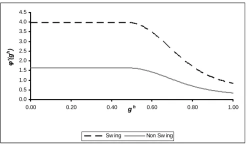
pthat φ0₁g1t

−φ0₂g2t

takes a given high value H, and a probability(1−p) that it takes a low valueL (H > L) . Suppose also thatφ0

1 g1 t −φ0 2 g2 t

is actually high (note that here we are evaluating φ0

h(·) at the current spending

level). Denote asEF R_lng1 t+1|g1t andEN F R_lng1 t+1|g1t

the expected value assigned by voters to their post-electoral utility under the incumbent in, respectively, the Fully Revealing equilibrium and the Non-Fully Revealing equilibrium. Equation (13a) implies that EF R_lng1

t+1|gt1

and EN F R_lng1

t+1|gt1

in the asymmetric case relate to one another according to EF Rlng1t+1|g 1 t = EN F Rlngt1+1|g 1 t + (1−p) ln1−Λg 2 tH 1−Λg2 tL < EN F Rlngt1+1 whereΛ=βρ0(·)EtL ΩINt+1−ΩOU Tt+1

expense of K. This result does not depend on voters assigning no value to K, only that there are some types of expenditure that voters as a whole value less than others, and these may be cut in an election year. The characterization ofKas total waste in the eyes of voters is simply an extreme way to capture those differences in the value assigned by voters to different goods and services provided by the government.

The government’s budget constraint now becomes

T =g_s1+g2_s+Ks s=t, t+ 1, . . . (24)

The voter’s problem is as described in section 3.2, except that here we assume, for simplicity, that voters in each region observe only their own g_th, but not that of the other region. The politician’s objective function is obviously different than in section 3.1. The incumbentL’s objective in a non-election yeart+ 1parallels (4) but with the addition of rents:

ΩIN_t+1(gL_t+1, L) =Z_tL₊₁¡gL_t+1¢+χ(Kt+1) +βEtL+1 ¡

ΩELE_t+2 (_·, L)¢ (25)

where rents χ are an increasing, weakly concave function ofK.19 _{The incumbent’s objective in the}

election yeart can then be written

ΩELE_t ¡gL_t, L¢=Z_tL¡g_tL¢+χ(Kt) +β ¡ ρ¡NL¢E_tLΩIN_t+1¡gL_t+1, L¢+¡1₋ρ¡NL¢¢E_tLΩOU T_t+1 ¢ (26) The differenceEt ¡ ΩIN_t+1−ΩOU T_t+1 ¢is (1 +β)¡πL₋πR¢2+E_tL¡Z_tL₊₁¡gL_t+1¢−Z_tL₊₁¡gR_t+1¢¢+ (1 +β)E_tLχ(Kt+1) +β2EtLΠt+3 (27)

but where the value inEtΠt+3 to being in office after t+ 2 includes the expected present discounted

value of future office rents in addition to ideology. Equation (27) represents four components in this model which make reelection valuable, three of which were present in (8): the ability to implement one’s preferred ideology; the ability to target expenditures to preferred regions; the rents from office; and the possibility that reelection attgives to win future reelection and hence gain future advantage of being in office.

With rents from holding office, the first-order condition in a non-election year for each region h

1 9_{Although politicians could differ in the value they place on rents relative to voters, we assume that all politicians}

assign the same value to such expenditures. Drazen and Eslava (2005) consider politicians who differ in the weight they put on voters relative to “rents”, where this weight is unobserved and all voters are homogeneous.