T
AINTED
M
ONEY
? C
ONTRIBUTION
L
IMITS AND
THE
E
FFECTIVENESS OF
C
AMPAIGN
S
PENDING
T
HOMAS
S
TRATMANN
CES
IFO
W
ORKING
P
APER
N
O
. 1044
C
ATEGORY2: P
UBLICC
HOICES
EPTEMBER2003
An electronic version of the paper may be downloaded • from the SSRN website: www.SSRN.com
CESifo Working Paper No. 1044
T
AINTED
M
ONEY
? C
ONTRIBUTION
L
IMITS AND THE
E
FFECTIVENESS OF
C
AMPAIGN
S
PENDING
Abstract
Campaign expenditures are not effective in increasing candidates’ vote shares if voters do not respond to the advertisement when they believe that campaign expenditures are financed with “tainted money.” In this situation, limiting contributions may reduce the number of policy favors that candidates promise to contributors, and thereby increase the effectiveness of campaign spending. Exploiting cross-state variation in campaign finance laws, this paper tests whether campaign expenditures by state House candidates are more productive in increasing vote shares when candidates run in states that limit contributions. The results show that campaign expenditures by incumbents, challengers, and open seat candidates are more productive when candidates run in states with campaign contribution limits, as opposed to in states without limits. Controlling for the endogeneity of incumbent spending, the study shows that in states with contribution limits, incumbent spending and challenger spending are equally productive, and that spending by both candidates is quantitatively important in increasing their vote shares.
JEL Code: D72.
Thomas Stratmann University of Chicago
Department of Economics, 1D3 Carow Hall 4400 University Drive
Fairfax, VA 22030-4400 U.S.A.
I would like to thank the National Science Foundation for financial support and participants of the brown bag lunch group at George Mason University, Cornell University, and the University of Maryland as well as Steve Coate, Dennis Coates, Dan Houser, and John Samples for helpful comments and suggestions. Stephen Daley provided excellent research assistance.
1
The other central issue is whether limits on contributions curtail free speech.
2
For example, in 2000 in Nixon v. Shrink the U.S. Supreme Court agreed with a district court that “large contributions raise suspicions of influence peddling tending to undermine citizens’ confidence "in the integrity of … government"” and that contribution limits are one way of upholding citizens’ confidence. This ruling was based on the 1976 Buckley v. Valeo decision which upheld contribution limits with the expressed hope that this would uphold or improve citizens trust in the integrity of government.
I. Introduction
At the center of the campaign finance reform debate is the concern that campaign contributions from private interests give rise to corruption and the appearance of corruption.1
This concern has motivated the U.S. Supreme Court to uphold contribution limits at the federal and state level. If contribution limits reduce the influence of contributors over policies or the perception of corruption, then contribution limits may change voters’ perception of the integrity of the political process – an explicit “hope” expressed by the courts upholding contribution limits.2
To date, there is scant evidence on whether contribution limits result in outcomes that are consistent with the hypothesis that contribution limits reduce voters’ perceptions of
corruption. This paper attempts to fill this void.
One of the central and somewhat puzzling findings in the academic literature on the effects of campaign advertisements on vote shares is that campaign expenditures have either no effect on the vote shares of challengers and incumbents (Levitt 1994, Palda and Palda 1998), or that challenger expenditures, and sometimes incumbent expenditures, have only a small effect on vote shares (Jacobson 1978, Green and Krasno 1988, Grier 1989, Coates 1998, Gerber 1998). (I will use the terms campaign contributions and campaign expenditures interchangeably,
3
http://www.cfinst.org/studies/vital/commentary.html
4
A separate empirical literature that examines whether contributions influence legislators decisions, correlates contributions with legislators’ voting behavior or time allocation (Chappel 1981, Kau et al. 1982, Hall and Wayman 1990, Durden et al. 1991, Evans 1986, Snyder 1992, Bronars and Lott 1997, Stratmann 1991, 1995, 2002, Ansolabehere, de Figueiredo, and Snyder 2003). This second strand of literature has produced mixed results. To date there is no
consensus to the extent that contributions result in quid-pro-quos, and thus changes in legislator behavior.
effective in increasing candidates’ vote shares is puzzling, given the apparent importance of spending large sums of money in electoral races. For example, in the 2000 elections candidates for the U.S. House of Representatives in competitive races spent between $2 million and $2.5 million and the average winner in Senate races spent $7.4 million.3
Recent theoretical models show that the productivity of campaign spending may be low when politicians trade policy favors for campaign contributions, because voters do not respond to campaign messages when they believe that the messages are financed with “tainted” money (Ashworth 2003, Coate 2003, Prat 2002a). Thus, small marginal effects of spending may have been found because voters do not respond to the advertisement when they believe that candidates trade policy favors for contributions.4
In this situation, contribution limits that lead to a reduction in policy favors make a candidate’s campaign advertisement more productive because voters attach more credence advertisements financed with “clean” money.
Previous empirical work may have found a low effectiveness of campaign spending because it did not account for the possibility that voters are less likely to vote for candidates who they believe to have promised policy favors to their contributors. This paper allows for the effectiveness of campaign spending to differ, depending on whether campaign spending is
puzzle regarding the effectiveness of campaign expenditures for incumbents’ and challengers’ vote shares.
To test the hypothesis that the effectiveness of contributions depends on whether campaign contributions are limited, federal U.S. data are not useful, as contribution limits to federal candidates are uniform for all candidates and have remain unchanged in nominal terms from 1976 until the recent federal 2002 legislation. This, however, is not the case with state campaign finance laws, which vary across states. State-level regulations provide the variation that allows one the hypothesis that campaign expenditures’ effectiveness depends on whether contributions are limited or not. This study therefore analyses the vote shares of candidates for state lower House races in states with and without contribution limits.
Any work on campaign expenditures has to address the issue that campaign expenditures are endogenous in the vote share equation because variables, such as unobserved district
partisanship or unobserved candidate quality are determining both the level of campaign
advertisements and the votes shares candidates receive. Much of the literature on this issue has focused on the likelihood that incumbent campaign expenditures are endogenous while
challenger expenditures are taken as exogenous. This study takes the same approach, but introduces a new instrument that identifies the effect of incumbent spending on his or her vote share. This instrument is the cost of advertising in the House district in which the incumbent runs for reelection. Advertising cost for media, such as television and radio advertisements determine campaign expenses, and if advertising cost are uncorrelated with district partisanship or incumbent quality, advertising cost is a valid instrument for campaign expenditures.
higher for all candidates when they run in states with campaign finance limits. This is the case for candidates in open seat races as well as for incumbents and challengers. The findings suggest that voter’s discount campaign advertising when they anticipate that candidates promised favors to interest groups in exchange for campaign contributions, and thus are consistent with the hypothesis that contribution limits reduce the perception of corruption.
In summary, this paper provides three contributions to the literature on the role of money in elections. It examines whether the results on the productivity of spending are consistent with the hypothesis that voters are less easily swayed by a campaign message when they believe that the candidate promised favors to interest groups in order to raise contributions. Further, it develops a new instrument for campaign spending which provides estimates for the productivity of incumbent spending, and using this instrument, the results show that in states with limits, the marginal product of spending is equated across incumbents and challengers. Finally, it examines this issue using state level data, which allow for a test of the proposed hypotheses using cross-state variation in campaign finance regimes.
Section II contains the theoretical framework that will guide the empirical analysis. The empirical research design is described in section III, and the data in section IV. I report results in section V, and section VI contains conclusions.
II. Conceptual Framework
A number of theoretical models predict that campaign contribution limits influence electoral outcomes. The results in these models depend on assumptions regarding the objective of candidates, the rationality of voters, the type of electoral competition, the goal of contributors,
5
This prediction that voters believe that politicians implement favors to contributors is consistent with less formal work by law scholars, who claim that campaign contributions have a corrupting influence on the political process (Lowenstein 1998). This corrupting influence in turn is thought to have a negative influence on voters perception of politics, and is thought to have a negative influence on their participation in the political process. Thus, even though legislators are not necessarily for sale, voters will perceive that legislators have a conflict of interest when they receive money from special interest groups (Lowenstein 1989).
6
Some empirical work finds that challenger spending sometimes reduces voters accuracy in correctly placing an incumbent on an ideological scale (Coleman and Manna 2000)
and the role of advertising in inducing voters to change their voting behavior. This section describes the main features of models (Pratt 2002a, Coate 2003, Ashford 2003) that predict that voters are less responsive to the campaign message, when they believe that candidates have obtained campaign funds by promising policy favors to contributors.5
A common strand in formal campaign advertising models is that candidates’
advertisements convey information to voters or that advertising provides a signal about candidate quality. It is assumed that the candidates do not disseminate lies about their qualities, and this assumption is probably a good first approximation, as if it were not, the opposing candidate would readily point out the lacking truth, and thus no candidate would have an incentive to disseminate lies.6
Voters are assumed to have priors about candidates’ positions or qualities, and campaign advertising allows voters to update their beliefs about candidate attributes. Thus, advertising provides a useful function in the political competition. It informs voters about candidate quality and about candidates’ characteristics.
In many of these candidate advertisement models, interest groups contribute because they expect policy favors from the candidate when elected, while candidates ideological position is assumed to be fixed (Coate 2003) or interest groups contribute because they want to move a
7
If the voter would automatically vote for the candidate who does not advertise, no candidate would advertise in equilibrium (Wittman 2002).
candidate’s platform closer to their own position (Prat 2002). While the empirical support for the assumption that interest groups and candidates engage in quid-pro-quos is mixed, this
assumption appears to be reasonable since contributors may have a stronger incentive to donate money to obtain a private good - a policy favor - as opposed to a public good - wanting the preferred candidate elected.
Voters know that candidates who do not advertise, do not advertise because they have no good information to disseminate about themselves, and thus are low quality candidates.
However, if a voter sees a campaign message from candidate A and no campaign message from candidate B, he does not automatically vote for candidate A, because he knows that candidate A promised at least some favors to the interest group in exchange for obtaining campaign funds.7
Thus, promising favors to contributors has a cost to candidates because voters are less likely to switch their vote to the advertising candidate because voters know that policy favors have been promised. Had fewer favors been sold, the campaign message would have been more
convincing, and the probability that the voter would switch his vote to the advertising candidate would have been higher.
Dollar limits on contributions can reduce the number of policy favors candidates promise to interest groups. While campaign contribution limits result in less campaign spending and reduce voters’ information about their voting options, limits also effect voters’ evaluation of candidates’ campaign messages because limits may decrease the number of favors candidates promise to contributors. Assuming that one candidate advertises and the other does not, the
probability that a voter will switch his vote to the advertising candidate will increase with limits if the beneficial effects of limits, i.e. fewer policy favor promises, outweigh their negative effects, i.e. the information loss (Coate 2003).
In light of the described theoretical model, the finding that campaign spending has little, if any, effect on vote shares at the national level (Levitt 1994, Palda and Palda 1998), may reflect that "the informational benefit of spending is offset by the policy bias needed to raise
contributions" (Prat 2002a, p. 182).
While the theory points to the possibility that campaign advertising may be more
productive when contributions are limited, the theory also shows that contribution limits may not have this effect if candidates are not inclined to promise many favors for votes, or when the loss of information about who is the “better” candidate, due to reduced advertisements, is sufficiently large (Coate 2003). Thus, the extent to which limits increase the productivity of campaign spending depends on how likely it is that candidates promise favors to contributors. If candidates tend to promise favors to contributors, then the empirical work is predicted to show that
campaign expenditures are more effective when limits are in place.
III. Research Design and Methods
Given that contribution limits do not vary across federal races, an analysis of expenditures by federal candidates will not reveal whether contribution limits can make campaign
expenditures more effective. Thus, this study examines the effectiveness of campaign advertising using state level data. Contribution limits differ among the states and this paper studies expenditure by candidates for state lower houses.
To analyze whether campaign contribution limits determine the effectiveness of campaign expenditures with respect to electoral outcomes, I will use the state House single member district as the unit of analysis. The empirical model is
VSijt =$0 + $1Ispendijt *Nolimitit + $2Ispendijt*Limitit + $3Cspendijt *Nolimitit +
$4Cspendijt*Limitit + $5Limitit + $6Partyijt + $7PevVSijt + (Xit + vt + ,ijt , (1)
where VSijt is the incumbent’s vote share in state i, and election year t and district j. The
variables Ispend and Cspend are incumbent and challenger campaign expenditures.
Limit is an indicator variable which equals one when the campaign finance law restricts individual contributions to candidates running in state House elections and zero otherwise.
Nolimit equals one if there are no restrictions on individual contributions and zero otherwise. Equation (1) differs from the campaign spending models in the earlier literature, because it interacts campaign expenditures with an contribution limit indicator. If incumbent spending is productive, then $1 is positive, and if challenger spending is productive, $3 is negative. The
theoretical model in section II predicts that $2 is positive and larger than $1 and that $4 is
negative and larger in absolute value than $3.
An alternative, but equivalent specification is to run the regression explaining incumbent votes shares with the levels of incumbent and challenger spending, and to interact spending by both candidates with the limit indicator (and no interactions with the nolimit indicator). This specification allows for the testing of whether there is a significant difference in the productivity of spending in limit versus non-limit states. The chosen specification (1) has the advantage of
readily showing the productivity of spending by challengers and incumbents in limit and no-limit states, and I will report whether $1 and $2 (as well as $3 and $4) are significantly different from
each other.
To be consistent with the previous literature on the effects of expenditures on vote shares, I include the variable PevVSijt which measures the historical electoral strength of the incumbent (the so-called normal vote). This variable serves as a measure of a district’s partisanship. I also include the Partyijt variable, which indicates the incumbent’s party affiliation (Jabcobson 1978, Green and Krasno 1988). I control for changes in national laws and national events that effect local elections via year fixed effects vt.
To control the for possibility that states with limits have a different political culture than those without limits, we include an indicator variable which measures whether a state has a limit on individual campaign contributions. Since this study is examining vote shares at the state level, the vector Xit includes state characteristics, which previous studies have found to be of
importance in explaining vote shares in state elections. The vector includes state per capita income, because voters tend to reward incumbents when they believe that they have helped them financially (Lowry, Alt and Ferree 1999). The vector of controls includes legislators’ salary, which is a measure of the professionalism of the legislature (for example Fiorina 1994, Moncrief 1999, Berry et al. 2000). In more professional legislatures incumbents have more resources to help them get reelected. The vector of state controls also includes an indicator for those states that implemented term limits for state House legislators, since term limits reduce the duration an individual can be a legislator, making public office less valuable (Grofman 1996). Another reason for including term limits is that the same political culture that led to the adoption of term
limits may have also led to the adoption of contribution limits. Thus, controlling for term limits is an additional control for variables that may simultaneously determine campaign contributions and election outcomes. Another control variable is an indicator variable measuring whether the state has an open primary election or not. I also include in the regression equation the share of the state popular vote received by the gubernatorial candidate and the presidential candidate who has the same party affiliation as the incumbent (or, in an alternative specification, the same party affiliation as the open seat candidate whose vote share is explained by the regression). These variables capture the political leanings of the constituency and also capture political tides (Berry et al. 2000). Previous studies have also included measures for redistricting but this is not
required here as no redistricting occurred between the elections (1996, 1998, and 2000) analyzed in this paper.
To control for the possibility that the effect of contributions is declining at the margin, I will employ the log of campaign spending as well as the square root of spending in addition to the linear functional form.
Suppose that the production function for vote shares has diminishing marginal returns (Mueller 1989), that states with contribution limits have lower levels of campaign spending than those without limits, and that the production function is the same across states. In this case, the regression analysis would detect different levels of campaign spending productivity because the marginal product of spending is higher in low campaign spending states with contribution limit than in high campaign spending states with no contribution limits, and not because voters are more responsive to the campaign message in states with contribution limits.
8
Examining the ratio of challenger spending to incumbent spending the difference in limit an non-limit state is not statistically significant at the 5 percent level or less.
marginal product of the percent increases is the same, regardless of the level of spending. This specification recognizes that a candidate’s marginal product of advertising is the same if he or she increases spending by ten percent starting from a base of $1,000, or by ten percent starting from a base of $100,000.
Another way of addressing the aforementioned issue is to examine the relative spending of incumbent and challengers. Suppose for a given election cycle the production function for an incumbent’s vote share is
, (2)
were vsin is the incumbent’s i vote share in state n and Pn is an indicator equaling one if the state
n has contribution limits and zero otherwise and assume that both incumbent and challenger
spending are productive, thus and . When "I equals "C and the 2s take
the assumed signs, then the first two terms of the production function collapse to ,
indicating that relative spending matters. A similar result holds for the last two terms of the production function. Expression the equation in logs we get
. (3)
In this formulation, relative spending matters for vote shares. This amounts to a log transformation of vote shares and contributions in equation (1).8
The hypothesis that campaign expenditures are most effective when limits are in place is easiest to test with expenditures in open seat races. In those races no incumbency advantage
9
Many unobserved variables determine vote shares. For example, vote shares are
influenced by whether political parties recruit more challengers, by independent expenditures, by party soft money, by leadership funds, and by incumbents’ war chests (Gierzynski and Breaux 1991, Epstein and Zemsky 1995, Milyo 1997, Milyo and Groseclose 1999, Hogan 2000, Gross, Goidel and Shields 2002). Unfortunately, much of this activity is not reported for candidates to state lower houses.
exists, thus the omitted variable bias, due to a lack of data on candidate quality is less severe. If candidate quality is randomly distributed among Democrats and Republicans, the coefficients on Republican and Democrat spending are not systematically biased.
For races with incumbents and challengers ordinary least square estimates from equation (1) and equation (3) may be biased without good measures of district partisanship and of
incumbent and challenger quality. Much of district partisanship as well as incumbent and
challenger quality are unobserved. This omitted variable bias may lead to an underestimation the effects of incumbent spending (see, for example, Jacobson 1978, Levitt 1994).9
The two-stage least square (2SLS) method provides unbiased estimates if the instruments used are exogenous. A valid instrument has to be correlated with the endogenous variable and uncorrelated with the error term in the second stage. Consistent with the previous literature, I will allow for the endogeneity of incumbent spending while assuming that challenger spending is exogenous.
Our instrument is the cost of media advertisement. Specifically, the instrument is the cost of radio advertisement. Candidates for state Houses use radio as one means of getting out their campaign message. The cost of this advertisement is one determinant of how much money candidates have to raise in order go to get out their campaign message. Our measure of
Quotations and Data, Inc. (SQAD), who collects radio advertising cost data for each of the Arbitron radio markets in the Untied States. The advertising cost data is “cost per point,” which is an estimate of the dollar amount required to deliver one rating point (or one percent of the audience) of any designated population within a spot market area. The radio advertising cost per point is from the 3rd quarter and measures the costs for 60 second units, for population aged 18 and above. In 2000, there were 267 Arbitron radio markets. The Arbitron markets are generally composed of metropolitan areas as defined by the federal government. I mapped state House congressional districts into these radio markets. The number of radio markets per state vary from one in the state of Alaska to twenty-one in the state of California. In 2000, the highest average cost is New York with a cost of $578 per rating point, while the lowest is in Montana with an average cost of $7.64 per rating point. With respect to single markets, in the year 2000 the highest cost of radio advertisement is in Los Angeles, California with $767 per rating point, while the lowest cost markets are in Billings, Montana, and Bismarck, North Dakota, with $5 per rating point.
For advertising cost to be a valid instrument, the cost measure has to be correlated with campaign expenditures. Some anecdotal and some systematic evidence suggests that political TV and advertising is a significant component of all campaign expenditures. At the federal level, for example, a headline the Washington Post claims that “In Presidential Race TV Ads were biggest ‘96 Cost By Far” (March 31, 1997, page A19). Systematic evidence is provides in Herrnson (2000) showing that TV and radio advertisements are a significant component of total campaign spending. Finally, PaineWebber analyst Leland Westerfield estimated that in 2000 TV broadcast advertisements reached $1 dollars and that radio, print and TV combined
10
http://www.bettercampaigns.org/freeairtime/monograph.pdf
11
I know of no data measuring TV and radio advertising expenditures as a fraction of total campaign expenditures for state Houses separately.
contribute to 80 percent of campaign expenses.10
This estimate includes presidential, federal, and state races.11
The results section will show that this instrument is positively correlated with advertising cost, thus meeting one requirement for a valid instrument. The other requirement is met if cost of radio advertisement is uncorrelated with candidate quality. This requirement if fulfilled if low quality incumbents do not tend to run for reelection in, for example, low advertising cost
districts.
IV. Data
Data on vote shares in general elections for state House single member districts in 1996, 1998 and 2000 come from each state’s Elections Division, or its State Board of Elections (Stratmann and Aparicio-Castillo 2002). I focus on single member districts since over 80 percent of all state legislators are elected to these districts, and because the theoretical models apply to these district types. Since at the federal level all House districts are single member districts, the focus on single member districts also makes it easier to transfer knowledge from the state to the federal level. Campaign contribution data to candidates in the 1996, 1998 and 2000 elections to state lower Houses come from the National Institute on Money in State Politics. Data on state characteristics were obtained from various issues of the Statistical Abstract of the United States. Since no systematic data are available on campaign expenditure at the state level,
12
That campaign expenditures closely track campaign contributions is also suggested by the statistic that only one percent of total campaign expenditures are self financed (Herrnson 2000).
13
Only four states (Colorado, Missouri, Oregon, and Idaho) moved from unrestricted contribution limits to contribution limits or vice versa between 1996 and 2000.
14
All categories of contribution limits tend to move together. That is, states that have strict contribution limits for individuals also have strict limits for unions and corporations.
we measure campaign expenditures by campaign contributions. Data at the federal level show that campaign contributions closely track campaign expenditures
(http://www.fec.gov/press/canye98.htm).12
The source for the campaign finance laws is the biannual publication, Campaign Finance Laws. States vary greatly in whether they have legal limits on campaign contributions by
individuals, PACs, corporations, unions, and parties (Stratmann and Aparicio-Castillo 2002). In this study I focus on individual limits, as they provide the largest source contributions to state candidates (Malbin and Gais, 1998).13
Another reason not to examine union or corporate contribution limits is that in some states union and corporate contributions are prohibited, and therefore prohibitions allow one to examine the effects of banning contributions, but not to study the effect of limiting but still allowing contributions, as is the goal of this paper.14
This data set includes thirty-seven of the fifty states. Since the empirical analysis focuses on single member districts, Arizona, New Jersey, and North Dakota are omitted from this data set. State legislators from these states run in multi-member districts. Similarly, Maryland and Vermont are excluded because their legislators run primarily in multi member districts. Nebraska is omitted because its elections are staggered. Louisiana is omitted as its relevant competition occurs in primaries, and sometimes there is no general election depending on the
outcome of the primary. No data or limited data were available for Alabama, Delaware, Iowa and South Dakota. Mississippi and Virginia are excluded because I focus on elections in 1996, 1998, and 2000 while the races in these states were in off election years.
V. Results
Table 1A reports means and standard deviation of variables used in the regressions with open seat candidates, and Table 1B does the same for regressions involving races with
incumbents. As with previous work, I do not include races where there was only one uncontested candidate. The open seat elections analyzed in the regression involve races that have two major party candidates, and the same holds for races with incumbents. Tables 1A and 1B show that approximately seventy percent of all races take place in states that have individual contribution limits. Democrats win open seat races with approximately fifty percent of the vote (Table 1A), while incumbents win contested races by obtaining on average sixty-six percent of the vote share (Table 1B). This shows that open seat races are more competitive than races with contested incumbents. Campaign spending by open seat candidates is roughly equal at $80,000. Spending in races with incumbents is uneven. Incumbents spent on average $87,900 in a race while their challengers spent $22,300.
Table 2 reports the results for open seat races when the dependent variable is the
Democrat’s vote share. The first three columns show the results when one does not account for the fact that the effectiveness of spending differs across races. The columns differ in that the first column uses linear spending to explain vote shares, the second column log spending, and the third column uses the square root of spending. The last three columns have the same three
Table 1A
Summary Statistics for Open Seat Races Mean (Standard Deviation) Percent of popular vote obtained
by Democrat 50.50 (13.49) Spending by Democratic Candidate 7.935 (20.374) Spending by Republican Candidate 7.891 (17.461) Percent of popular vote received
by a Democrat in the previous election
44.65 (30.14)
Contribution limit for individuals=1, 0 otherwise
0.702 (0.458) Professionalism in legislature
(Legislator salary per days in session), in hundreds of dollars
2.762 (2.055)
Open primary=1, 0 otherwise 0.511
(0.500) Percent of popular vote of
presidential candidate with the same party affiliation as the incumbent - if presidential election
46.24 (7.156)
Percent of popular of
gubernatorial candidate with the same party affiliation as the incumbent - if gubernatorial election
43.53 (13.24)
State per capita income, in thousands of dollars
15.777 (2.118)
Term limit=1, 0 otherwise 0.604
(0.496)
N 1,246
Notes: Campaign expenditures in real 2000 dollars. Measured in 10,000 of dollars. Data are for races to state lower Houses, 1996-2000.
Table 1B
Summary Statistics for Races with Incumbents Mean (Standard Deviation)
Percent of popular vote obtained by the Incumbent 65.60 (11.19) Incumbent spending 8.785 (30.72) Challenger spending 2.231 (6.480)
Incumbent is Democrat=1, 0 ow. 0.515
(0.500)
Percent of popular vote in previous election 69.72
(16.67) Contribution limit for individuals=1, 0
otherwise
0.714 (0.452) Professionalism in legislature (Legislator
salary per days in session), in hundreds of dollars
2.926 (2.082)
Open primary=1, 0 otherwise 0.547
(0.498) Percent of popular vote of presidential
candidate with the same party affiliation as the incumbent - if presidential election
47.11 (8.169)
Percent of popular of gubernatorial candidate with the same party affiliation as the
incumbent - if gubernatorial election
45.42 (14.71)
State per capita income, in thousands of dollars 16.063
(2.288)
Term limit=1, 0 otherwise 0.438
(0.496) Cost of radio advertising, in thousands of
dollars
83.46 (116.6)
N 3,962
Notes: Campaign expenditures measured in 10,000 of dollars in real 2000 dollars. Data are for races to state lower Houses, 1996-2000.
Table 2
Explaining Vote Shares of Open Seat Candidates
Robust Standard Errors in Parentheses below Coefficient Estimates
Dependent variable vote
share ln(vote share) vote share vote share ln(vote share) vote share (i) linear spending (ii) log spending (iii) square root spending (iv) linear spending (v) log spending (vi) square root spending Constant 15.65 (3.485) 3.384 (0.072) 19.13 (3.326) 17.07 (3.073) 3.275 (0.076) 20.19 (3.105) Spending by Democrat 0.176 (0.041) 0.133 (0.019) 2.849 (0.700) Spending by Republican -0.256 (0.068) -0.131 (0.022) -3.712 (0.882) Democrat spending in
states without limits ($1)
0.134 (0.011) 0.119 (0.018) 2.160 (0.308) Democrat spending in
states with limits ($2)
0.606 (0.168) 0.155 (0.013) 5.206 (0.763) p-value that $2 $1 0.001 0.001 0.001 Republican spending in states without limits ($3)
-0.201 (0.024) -0.105 (0.020) -2.862 (0.426) Republican spending in
states with limits ($4)
-0.693 (0.166) -0.163 (0.014) -6.103 (0.882) p-value that |$4| |$3| 0.001 0.001 0.001
Vote share of Democrat in previous election 0.239 (0.021) 0.003 (0.0004) 0.205 (0.019) 0.227 (0.020) 0.003 (0.0003) 0.194 (0.018) Contribution limit for
individuals=1, 0 otherwise -0.760 (0.558) 0.019 (0.014) -0.530 (0.653) -0.010 (0.761) 0.054 (0.032) 0.429 (1.446) Professionalism in legislature (Legislator salary per days in session) 0.198 (0.218) -0.005 (0.004) 0.285 (0.264) 0.399 (0.224) -0.004 (0.005) 0.460 (0.269) Open primary=1, 0 0.423 0.010 0.620 0.550 0.014 0.739
otherwise (0.704) (0.012) (0.660) (0.640) (0.013) (0.740) Vote share of gubernatorial election -if gubernatorial election -0.005 (0.018) -0.0005 (0.0003) -0.015 (0.017) -0.018 (0.016) -0.0006 (0.0003) -0.027 (0.014) Vote share of presidential candidate -if presidential election 0.379 (0.058) 0.007 (0.001) 0.365 (0.051) 0.363 (0.051) 0.007 (0.001) 0.350 (0.048)
State per capita income 0.477
(0.168) 0.009 (0.003) 0.446 (0.175) 0.386 (0.141) 0.009 (0.004) 0.365 (0.166) Term limit=1, 0 otherwise -0.036 (0.601) 0.004 (0.009) -0.022 (0.583) 0.456 (0.519) 0.008 (0.009) 0.379 (0.532) Indicators for election
cycles YES YES YES YES YES YES
R-squared 0.46 0.59 0.53 0.48 0.60 0.56
Notes: N=1,266. The dependent variable is the Democrat’s vote share in a race to a state lower House in the 1996, 1998, and 2000 general elections. Expenditures are measured in 100,000 of (real 2000) dollars.
alternative specifications, but allow for the effectiveness of spending to differ, depending on whether candidates face contribution limits or not. Whenever the regression includes log spending, the dependent variable is the log of the vote share (Table 2, columns 2 and 5) instead of the vote share itself. As shown in equation (3), this specification implies estimating the effect of relative spending on vote shares. In the other specifications the dependent variable is the untransformed vote share.
The first three columns of Table 2 indicate that the marginal product of spending is larger Republicans than for Democrats. A $10,000 increase in spending increases the popular vote by
0.18 percentage points for Democrats and by 0.26 percentage points for Republicans, and this difference in the marginal product of spending is statistically significant at the five percent level (Table 2, column 1). When estimating the regression with the square root of spending, campaign spending remains productive for both Democrats and Republicans and the difference in the productivity of spending between Republicans and Democrats remains statistically significant (Table 2, column 3). When evaluated at the mean spending levels, the point estimates associated with the square root of spending imply that a $10,000 increase in spending increases
Republicans’ percent at the polls by 0.7 percentage points and Democrats’ percent by 0.5
percentage pints. However, the log-log specification shows that the elasticity of spending is equal for both party members. Here, a one percent increase in spending results in a 0.13 percentage increase in the popular vote. Evaluated at the mean, a one percent increase in spending equals almost $800, and a percentage change by 0.12 percent implies an increase of 0.065 percentage points in the popular vote. Thus, open seat candidates must spent about $12,000 to increase their vote share by one percent.
While the regression explains forty-six percent of the variation when linear spending is employed, the R-square increases to fifty percent in the square root specification and to fifty-one percent in the log-log specification. The fact that regression produces a better fit in the non-linear specifications suggests that campaign spending is subject to diminishing marginal returns.
For consistency, the regression with open seat races uses all of the control variables that will be used in the regression with incumbents. Among the control variables, the vote share of the Democratic candidate in the previous vote share has the anticipated positive sign and is statistically significant. Among the remaining control variables, only the vote share of the
15
That some of the covariates are not statistically significant is perhaps not surprising because these variables were hypothesized to be important in determining incumbents’ vote shares, not vote shares of open seat candidates. However, I included these covariates in the open seat regressions to allow for comparability between open seat regressions and regressions with incumbents.
democratic presidential candidate and state per capita income have consistently the same sign regardless of specification and are statistically significant.15
Those results show the existence of coattail effects and that Democrats in open seat races do better in elections when state per capita income is high. Vote shares in open seat races are not affected by term limits, the gubernatorial vote share, whether the primary is open, whether the state has contribution limits, and by the professionalism of the legislature. The point estimates on the campaign expenditure variable are robust to alterative specifications. For example, the coefficients on the campaign expenditures by Democrats and Republicans do not change by much, either quantitatively or qualitatively, when we exclude the state control variables.
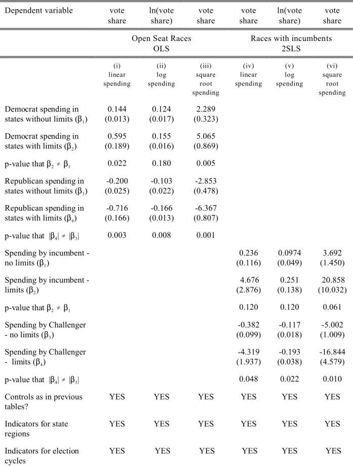
The last three columns of Table 2 tests the hypothesis that campaign spending is more productive in increasing votes in states with contributions limits. For states without contribution limits, the effectiveness of linear spending is estimated as 0.13 percentage points per $10,000 campaign expenditure for Democrats and as 0.20 percentage points for Republicans. Limits increase the productivity of spending to 0.6 percent for Democrats and 0.7 percent for
Republicans. Thus, spending is over three times as productive in states with contribution limits than in states without these limits, and this difference in the productivity is statistically
significant for both Democrats and Republicans. Using log-log specification, the elasticity point estimate indicates that a one percent increase in campaign expenditures increases the vote shares by approximately 0.11 percent in states without limits and approximately 0.16 in states with
16
When adding state fixed effects to the regression in Table 2, many of the standard errors approximately double in size. However, the point estimates remain statistically significant, and their magnitudes are similar to the magnitudes of the coefficients wen no fixed effects are added to the regression. Thus the inclusion of state fixed effects leaves the conclusions unaltered. contribution limits. Relative to the linear specification, we find qualitatively similar but quantitatively larger effects when we run the regression using the square root transformation of campaign contributions. In the square root specification candidates in limit-states receive between 0.9 and 1.0 extra percentage points for an additional increase of $10,000 in spending, when evaluated at the mean spending level. The first three columns of table A2 in the appendix report open seat regression results when nine regional indicators are added to the regression equation. The point estimates and t-statistics are similar to those reported in Table 2.16
The results from the open seat regressions lend support to the hypothesis that voters are less likely to respond to advertising when contribution limits curtail the amount of money a candidate can seek from contributors. The productivity of contributions is significantly higher in states with limits than in states without limits. Next, I will examine the effect of campaign spending in races with incumbents.
The OLS results in the first three columns of Table 3 show that the coefficients on incumbent and challenger spending are quantitatively and qualitatively similar to those in
previous literature: the effect of incumbent spending is negative and not different from zero, and challenger spending is productive in reducing the incumbents’ vote shares. For challengers a 10,000 increase in spending increases vote shares by 0.4 percentage points (Table 4, column 1). The log-spending and the square root of spending specifications also show that incumbent spending is ineffective in increasing incumbents’ vote shares but that challenger spending is
Table 3
Explaining Vote Shares Incumbents Ordinary Least Square Estimates
Robust Standard Errors in Parentheses below Coefficient Estimates
Dependent variable vote
share ln(vote share) vote share vote share ln(vote share) vote share (i) linear spending (ii) log spending (iii) square root spending (iv) linear spending (v) log spending (vi) square root spending Spending by Incumbent -0.004 (0.004) 0.0096 (0.0058) 0.002 (0.141) Spending by Challenger -0.435 (0.012) -0.107 (0.009) -4.762 (0.783) Spending by incumbent - no limits ($1) -0.007 (0.006) -0.009 (0.005) -0.249 (0.134) Spending by incumbent - limits ($2) 0.070 (0.039) 0.025 (0.007) 1.021 (0.353) p-value that $2 $1 0.051 0.001 0.001 Spending by Challenger - no limits ($3) -0.315 (0.077) -0.088 (0.011) -3.526 (0.594) Spending by Challenger - limits ($4) -1.202 (0.159) -0.125 (0.007) -7.493 (0.644) p-value that |$4| |$3| 0.001 0.005 0.001 Incumbent is Democrat=1, 0 ow. 1.920 (0.504) 0.026 (0.007) 1.897 (0.477) 1.918 (0.521) 0.026 (0.007) 1.893 (0.501) Vote share in previous
election 0.269 (0.026) 0.003 (0.0003) 0.230 (0.024) 0.255 (0.025) 0.003 (0.0003) 0.222 (0.023) Contribution limit for
individuals=1, 0 otherwise -2.319 (0.915) -0.032 (0.011) -2.586 (0.844) -1.057 (0.909) -0.065 (0.017) 0.421 (1.538) Professionalism in legislature (Legislator salary per days in session) 0.836 (0.298) 0.011 (0.003) 0.912 (0.279) 0.828 (0.287) 0.012 (0.003) 0.856 (0.266)
Open primary=1, 0 otherwise -0.565 (0.805) 0.011 (0.010) -0.045 (0.767) -0.295 (0.804) 0.009 (0.009) -0.086 (0.690) Vote share of presidential candidate -if presidential election 0.217 (0.033) 0.003 (0.0004) 0.200 (0.031) 0.208 (0.030) 0.003 (0.0004) 0.195 (0.028) Vote share of gubernatorial election -if gubernatorial election 0.004 (0.008) 0.0001 (0.0002) -0.001 (0.008) 0.0009 (0.008) 0.0002 (0.0002) -0.005 (0.009)
State per capita income 0.667
(0.222) 0.010 (0.003) 0.660 (0.235) 0.663 (0.223) 0.010 (0.003) 0.653 (0.223) Term limit=1, 0 otherwise 0.532 (0.702) 0.009 (0.010) -0.007 (0.679) 0.648 (0.706) 0.010 (0.009) 0.018 (0.631) Indicators for election
cycles YES YES YES YES YES YES
R-squared 0.36 0.49 0.40 0.39 0.49 0.38
Notes: N=3,962. All standard errors are adjusted to allow for non-independence of observations within a state. The unit of observation is a race to a state lower House in the 1996, 1998, and 2000 general elections. Expenditures are measured in 10,000 of (real 2000) dollars.
effective to increase challengers’ vote shares. For example, the square root specification indicates that a challenger’s vote share rises by 1.6 percentage points when he or she spends an extra $10,000.
Comparing the state-level OLS results for incumbent and challenger spending (Table 3, columns 1 to 3) with the federal-level OLS results in previous studies, one notices that the federal studies report somewhat similar effects of incumbent and challenger campaign
expenditures on vote shares. For example, Jacobson (1980) reports that $100,000 in spending increases challengers vote share by 2.7 percentage points using OLS estimation, while incumbent
expenditures are ineffective in increasing incumbents’ vote shares. Green and Krasno’s (1988) OLS results imply that $100,000 spending translates into a 0.1 percent vote share increase for incumbents and 1.6 percentage point increase for challengers. The first three columns of Table 3 show that spending by incumbents of state Houses is as unproductive as incumbents’ spending at the federal level, while spending by state challengers is somewhat more productive (a 0.4 percentage point increase for an extra $10,000 increase in spending, Table 3, column 1) than spending by U.S. House of Representative challengers (a 1.6 to 2.7 percentage point increase for a $100,000 increase in spending).
Among the control variables in Table 3, the vote share in the previous elections is statistically significant in all regressions, suggesting that partisan leanings are important in explaining election outcomes. All specifications indicate that Democrat incumbents, on average, receive about two percentage points more at the polls than Republican incumbents. The
hypothesis that a more professional legislature helps incumbents receive a larger vote share finds support in all specifications. Further, lower incumbents’ vote shares are associated with
campaign contribution limits. However, term limits have no statistically significant effect on incumbents’ vote shares. The coefficients on state per capita income are always positive and statistically significant, indicating that incumbents are doing better at the polls when voters are doing well in terms of per capita income. Whether incumbents run for reelection in states with or without open primaries does not affect their vote shares. Finally, the results show that coattail effects exist with respect to votes cast in presidential races, but not with respect to votes cast in gubernatorial races. An increase in the presidential candidate’s popular vote by one percentage point results in a 0.2 percentage point increase in the incumbent’s vote share when he or she
belongs to the same party as the presidential candidate.
The last three columns of Table 3 show the OLS estimation results when one allows for the productivity of incumbent and challenger spending to differ according to whether contribution limits curtail their fundraising ability or not. In all three specifications, incumbent spending is
ineffective in increasing their vote shares when they run for reelection in states without
contribution limits; the coefficients are negative and statistically insignificant. However, in all specifications incumbent spending is productive in helping them get reelected when they run in states with contribution limits. The difference in the productivity of incumbent spending in states with and without limits is statistically significant in all three specifications. The result from the linear specification shows that a $10,000 increase in incumbent spending leads to an almost 0.1 percentage point increase in the popular vote, while the square root specifications indicates an increase by 0.17 percentage points, when evaluated at the mean incumbent spending.
Challenger spending remains more productive than incumbent spending (Table 3,
columns 4 to 6). Similar as incumbent spending, challenger spending is more productive in states with contribution limits. The difference in the productivity of spending is statistically significant regardless of whether the contribution variable is measured in linear form, as the log, or as the square root. While the magnitude of the point estimates on incumbent spending in states with contribution limits remains small, the result for challenger spending in states with limits implies that a $10,000 increase in spending increases vote shares between 1.2 percentage points (Table 3, column 4) and 2.5 percentage points (Table 3, column 6). The log-log specification results show that a one percent increase in challenger spending in contribution limit states increases their vote shares by 0.13 percent. Challengers’ vote shares increase by 0.09 percent in states without
contribution limits.
Consistent with the theoretical models, incumbent contributions and challenger contributions are more effective in increasing vote shares when they face contribution limits. Similar as some of the previous literature, these regression results suggest that the marginal effect of incumbent spending is significantly lower than that of the challenger. To further investigate this issue I estimate the regression in Table 3 with 2SLS.
Table 4 reports the 2SLS estimates, controlling for the endogeneity of incumbent campaign spending. The corresponding first stage estimates show that advertising costs are a statistically significant determinant of campaign spending. A one-thousand dollar rise in the cost per rating point increases incumbent spending by eighteen percent (Table A1). Thus, the
instrument is valid with respect to being able to explain variation in the endogenous incumbent campaign spending variable.
The first three columns of Table 4 show the 2SLS estimates when no distinction is made between candidates running in states with and without contribution limits. Incumbent spending has now a positive sign in all three specifications and the productivity of spending increases more than ten fold relative to the corresponding regressions in Table 3, however the point estimates remain statistically insignificant. Challenger spending remains statistically significant and the magnitudes of the 2SLS point estimates increase by approximately fifty percent. The regressions show that the advertising instrument works in the way that was anticipated: OLS underestimates the effect of incumbent campaign spending. A Republican incumbent running for reelection in a district with unobserved preferences for a Republican representative, for example, will receive a high vote share even if he or she has few campaign expenditures. This unobserved and thus
Table 4
Explaining Vote Shares Incumbents Two Stage Least Squares Estimates
Robust Standard Errors in Parentheses below Coefficient Estimates
Dependent variable vote
share ln(vote share) vote share vote share ln(vote share) vote share (i) linear spending (ii) log spending (iii) square root spending (iv) linear spending (v) log spending (vi) square root spending Spending by Incumbent 0.331 (0.319) 0.096 (0.062) 4.597 (3.749) Spending by Challenger -0.642 (0.314) -0.141 (0.030) -7.324 (2.735) Spending by incumbent - no limits ($1) 0.205 (0.111) 0.053 (0.022) 2.482 (1.054) Spending by incumbent - limits ($2) 3.418 (1.233) 0.165 (0.047) 14.578 (4.363) p-value that $2 $1 0.001 0.001 0.002 Spending by Challenger - no limits ($3) -0.397 (0.110) -0.108 (0.016) -4.787 (1.043) Spending by Challenger - limits ($4) -3.910 (0.882) -0.188 (0.019) -15.949 (2.420) p-value that |$4| |$3| 0.001 0.001 0.001 Incumbent is Democrat=1, 0 ow. 1.598 (0.607) 0.025 (0.009) 1.717 (0.627) 2.134 (1.633) 0.026 (0.010) 1.906 (1.039) Vote share in previous
election 0.276 (0.031) 0.003 (0.0003) 0.239 (0.029) 0.239 (0.035) 0.003 (0.0003) 0.208 (0.027) State controls as in Table 3?
YES YES YES YES YES YES
Indicators for election cycles
YES YES YES YES YES YES
Notes: N=3,962. All standard errors are adjusted to allow for non-independence of observations within a state. The unit of observation is a race to a state lower House in the 1996, 1998, and 2000 general elections. Expenditures are measured in 10,000 of (real 2000) dollars.
omitted variable causes downward bias on the coefficient associated with incumbent spending. The results in Table 4 are consistent with the hypothesis that OLS introduces a downward bias in incumbent spending productivity.
The first three columns of table 4 show that incumbent spending remains less productive than challenger spending. A simple comparison of the point estimates indicates that challenger spending is approximately twice as productive as incumbent spending. Next, I will examine whether this difference in productivity disappears when allowing for the effectiveness of spending to differ by whether candidates run in states with or without contribution limits.
The last three columns of table 4 report the 2SLS results when one allows the
productivity of spending to differ depending on whether candidates run in states with or without contribution limits. The results now show that spending is productive for incumbents in both types of states, although incumbents’ productivity of spending is significantly higher when they run in states that limit contributions. A $10,000 increase in spending increases incumbents’ vote share by 0.2 percentage points in states with limits and by 3.4 percentage points in states without limits (Table 4, column 4). The corresponding percentage point changes for the square root specification are 0.4 and 2.5 percentage points. In all specifications the difference in spending productivity between both incumbent types is statistically significant.
As in Table 3, the results show that challenger spending is more productive in states with limits than without limits. Relative to the OLS estimates, Table 4, columns 4 to 5 show that all point estimates are larger when estimating the regression equation with 2SLS. In the linear specification the estimates show that challenger spending is almost ten times more productive in garnering votes in states with limits than in states without limits, while the square root
17
Related to this finding is the study by Gerber (1998) who found that challenger and incumbent spending in U.S. Senate races is equally productive.
specification indicates that spending is three times more productive in states with limits. The magnitudes of the 2SLS coefficients in the log-log specification also increased relative to the OLS estimates. The results show that the increasing expenditures by one percent leads to a 0.17 percent increase in the vote share for incumbents and a 0.19 percent increase for challengers when they run in states without contribution limits.
The 2SLS results show that challenger spending is approximately as productive as
incumbent spending when both candidates run in states with contribution limits. The coefficients on spending by both candidates are not statistically different from each other, and thus we can not reject the hypothesis that their spending productivity is equal in absolute value.17
Interestingly, in states without contribution limits challenger spending is almost twice as productive as
incumbent spending, and this difference is statistically significant in all three specifications (Table 4, column 4 to 6).
For comparison, Jabcobson’s (1980) 2SLS results show that challengers’ vote shares increase by 4.2 percentage points using 2SLS, while incumbent expenditures are ineffective in altering vote shares. Green and Krasno’s (1988) 2SLS estimates imply that $100,000 spending translates into a 2.4 percent vote share increase for incumbents and a 2.2 percentage point increase for challengers. The estimates for contribution limit states reported in this study are larger than the previously reported estimates, up to one order of magnitude. For example, Table 4, column 4 indicates that a $10,000 increase in incumbent spending increases their vote shares by 3.4 percentage points, and that a corresponding increase in challenger spending results in a 3.9
percent increase. However, when candidates run in states without contribution limits, a $10,000 increase in spending results in a 0.2 percent increase in vote shares for incumbents and a 0.4 percent increase for challengers, which is similar to the findings in the previously mentioned studies at the federal level.
VI. Conclusions
This paper shows that campaign advertising is more productive when contributions are limited, as opposed to unlimited. In races that are subject to contribution limits, an extra $10,000 in challenger spending increases his or her vote share by up to 4 percent, and the same increase in incumbent spending raises the incumbent’s vote share by 3.4 percent. However, in races not subject to contribution limits, the same increase in spending raises challengers’ vote shares by 0.4 percent and incumbents’ vote shares by 0.2 percent. While incumbents’ and challengers’ campaign spending is equally productive when they run in states that limit
contributions, challengers’ spending is more productive than incumbents’ spending when they run in states without contribution limits. In open seat races that are subject to contribution limits, a $10,000 spending increase raises vote shares by up to 1 percentage point, while the same
increase in spending raises their votes shares only between 0.4 and 0.5 percentage points when the candidates are not subject to contribution limits. These results demonstrate that campaign advertising is more productive when contributions are limited, as opposed to unlimited.
That the results in this paper show that campaign spending is productive helps resolve the long standing question of why candidates spend money on advertising when it appears that this is not effective in garnering votes. These results suggest that previous work found low productivity
of campaign spending because its research design did not allow for productivity of spending to differ across campaign finance regulations.
The results are consistent with the theoretical models that voters are less responsive to campaign advertisements when contributions are unlimited because they believe that candidates who run in states where contributions are unlimited have promised many favors to contributors. Thus the findings are consistent with the hypothesis that contribution limits reduce the perception of corruption. The regression results document a smaller marginal impact of political advertising when campaign contributions are unlimited than when contributions are limited, which suggests that voters believe that more policy favors are promised when contributions are unlimited. However, the nature of the data employed does not allow one to obtain direct evidence that candidates trade contributions for policy favors.
The marginal product of incumbent and challenger spending is equal in states with
contribution limits and in these states campaign spending is an effective means of increasing vote shares. Productivity of spending is significantly smaller in states with contribution limits for both incumbents and challengers. Interestingly, we find that even at this lower level of productivity in states without contribution limits incumbent spending is less effective in increasing vote shares than challenger spending.
References
Ansolabehere, Stephen ,John M. de Figueiredo and James M. Snyder Jr. “Why is There so Little Money in U.S. Politics?” Journal of Economic Perspectives, 17, 1, Winter 2003 pp.???
Ashworth, Scott, “Campaign Finance and Voter Welfare with Entrench ed Incumbents,” mimeo, 2002, Harvard University.
Austen-Smith, David, “Interest Groups, Campaign Contributions and Probabilistic Voting, ” Public Choice, 1987, 54, 123-39.
Bailey, Michael, Money and Representation: An Exploration in Multiple Dimensions with Informative Campaigns,” mimeo, Georgetown University, 2002.
Berry, William D., Michael B. Berkman and Stuart Schneiderman, “Legislative Professionalism and Incumbent Reelection: The Development of Institutional Boundaries, American Political Science Review, 94, 4, December 2000, p.859–74.
Coate, Stephen, “Political Competition with Campaign Contributions and Informative Advertising,” 2003,” mimeo, Cornell University.
Coate, Stephen, “Power-hungry Candidates, Policy Favors, and Pareto Improving Campaign Finance Policy,” mimeo, Cornell University, 2003.
Coates, Dennis “Additional Incumbent Spending Really Can Harm (at Least Some) Incumbents: An Analysis of Vote Share Maximization” Public Choice, v95, n1-2, April 1998, 63-87. Coleman, John and Paul Manna, “Congressional Campaign Spending and the Quality of
Democracy,” Journal of Politics, 62, 3, 2000, pp.757-789.
Daniel, Kermit and John R. Lott, "Term Limits and Electoral Competitiveness: Evidence from California's State Legislative Races," Public Choice 90, 1997, 165-84.
Evans, Diana M. (1986). PAC contributions and roll-call voting: Conditional power, in A.J. Cigler and B.A. Loomis (eds.), Interest Group Politics, 2nd ed., Washington, D.C.: Congressional Quarterly.
Epstein, David and Peter Zemsky, “Money Talks: Deterring Quality Challengers in Congressional Elections,” American Political Science Review, 89, 1995, 295-308.
Feigenbaum, Edward D. and James A. Palmer, Campaign Finance Law, Federal Election Commission, bi-annual issues, 1980-2000.
Fiorina, Morris “Divided Government in the American States: A Byproduct of Legislative Professionalism,” American Journal of Political Science, June 1994, 88, pp.304-16.
Garand, James C. “Electoral Marginality in State Legislative Elections, 1968-1986,” Legislative Studies Quarterly, February 1991, pp. 7-28.
Gerber, Alan "Estimating the Effect of Campaign Spending on Senate Election Outcomes Using Instrumental Variables", American Political Science Review, 1998, 92, pp.401-11. Gierzynski, Anthony, and David Breaux, “Money and Votes in State Legislative Election,”
Legislative Studies Quarterly, 1991, 16, 203-17.
Green, D. and Krasno, J. “Salvation of the Spendthrift Incumbent: Reestimating the effects of campaign spending in House elections,” American Journal of Political Science, 32, 1988, 884-907.
Grier, Kevin B. “Campaign Spending and Senate Elections, 1978-84” Public Choice, 63(3), 1989, 201-220.
Gross, Donald A., Robert K. Goidel, and Todd G. Shields, “State campaign finance regulations and electoral competition, March 2002, American Politics Research, 30, 2, 143-65.
Grossman Gene M. and Elhanan Helpman, "Electoral Competition and Special Interest Politics, "
Review of Economic Studies, 63: 265-286, 1996.
Hall, Richard and Wayman, Frank. “Buying Time: Moneyed Interests and the Mobilization of Bias in Congressional Committees.” American Political Science Review 84 (1990): 797-820. Herrnson, Paul, Congressional Elections: Campaigning at Home and in Washington, Washington,
D.C.: CQ Press, 3rd ed. 2000.
Hogan, Robert, “The Costs of Representation in State Legislatures: Explaining Variations in Campaign Spending,” Social Science Quarterly, December 2000.
Jacobson, Gary C., “The Effects of Campaign Spending on Congressional Elections,” American Political Science Review, 72, 1978, 469-91.
Jacobson, Gary C. “The Marginals Never Vanished: Incumbency and Competition in Elections to the U.S. House of Representatives, 1952-1982,” American Journal of Political Science, February 1987, 31, pp. 126-41.
Jacobson, Gary C., The Politics of Congressional Elections, 4th
Edition, New York: Longman, 1997. Kau, James B., Donald Keenan, and Paul H. Rubin, “A general equilibrium model of congressional
voting.” Quarterly Journal of Economics, 97, 1982, 271-293.
Krasno, Jonathan and Donald Philip Green, “Preempting Quality Challengers in House Elections,”
Levitt, Steven. “Using Repeat Challengers to Estimate the Effect of Campaign Spending on Election Outcomes in the U.S. House.” Journal of Political Economy 103, August 1994, 777-98.
Lowenstein, Daniel H. “On Campaign Finance Reform: The Root of All Evil is Deeply Rooted (Frameworks of Analysis and Proposals for Reform: A Symposium on Campaign Finance), 1989, 18, Hofstra Law Review, 301-67.
Lowry Robert C., James E. Alt and Karen E. Ferree, “Fiscal Policy Outcomes and Electoral
Accountability in the American States,” American Political Science Review, December 1999, 92, pp.759-74.
Malbin, Michael J. and Gais, Thomas L., The Day After Reform: sobering campaign finance lessons from the American states. Rockefeller Institute Press, 1998.
Milyo, Jeffrey The Economics of Campaign Finance: FECA and the Puzzle of the Not Very Greedy Grandfathers, Public Choice, 1997, 93, 245-270.
Milyo, Jeffery and Timothy Groseclose, "The Electoral Effects of Incumbent Wealth," Journal of Law and Economics, 42(2), October 1999, 699-722.
Moncrief, Gary F. Recruitment and Retention in U.S. Legislatures,” Legislative Studies Quarterly, May 1999, 24, pp. 173-208.
Ortuno-Ortin, Ignacio and Christian Schultz,“Public Funding for Political Parties,” CESifo Working Paper No. 368, 2000.
Osbourne, Martin J. and Al Slivinski, "A Model of Political Competition with Citizen Candidates",
Quarterly Journal of Economics, 1996, 111(1), 65-96.
Palda Filip and Kristian Palda, “The Impact of Campaign Expenditures on Political Competition in the French Legislative Elections of 1993, Public Choice, 94, 1998, pp.157-174.
Potters, Jan, Randolph Sloof and Frans van Winden, “Campaign Expenditures, Contributions, and Direct Endorsements: The Strategic Use of Information and Money to Influence Voter Behavior,” European Journal of Political Economy, 1997, 13, 1-31.
Prat, Andrea,, “Campaign Spending with Office-Seeking Politicians, Rational Voters, and Multiple Lobbies,” Journal of Economic Theory, 2002a, 103(1), 162-189.
Prat, Andrea, “Campaign Advertising and Voter Welfare,” Review of Economic Studies, 2002b 69(4), 999-1018.
Smith, Bradley A. "Campaign Finance Regulation: Faulty Assumptions and Undemocratic Consequences" Cato Policy Analysis no. 238, September 13, 1995.
Sorauf, Frank J., Inside Campaign Finance, Myths and Realities. Yale University Press, 1992
SQAD Media Market Guide, Spring 1996, Spring 1998, and Spring 2000.
Stratmann, Thomas, “What Do Campaign Contributions Buy? Deciphering Causal Effects of Money and Votes.” Southern Economic Journal, 57, 1991, 606-64.
Stratmann, Thomas, "Campaign Contributions and Congressional Voting: Does the Timing of Contributions Matter?" Review of Economics and Statistics, February 1995, 72 (1). Stratmann, Thomas "Can Special Interests Buy Congressional Votes? Evidence from Financial
Services Legislation." Journal of Law and Economics, 45(2), October 2002, 345-74. Stratmann Thomas, and Francisco J. Aparicio-Castillo “Competition Policy for Elections: Do
Campaign Contribution Limits Matter?” mimeo, George Mason University 2002.
Thompson, Joel A. and Moncrief, Gary F., eds. Campaign Finance in State Legislative Elections.
Congressional Quarterly Books, 1998.
Wittman, Donald “Rational Voters and Political Advertising” mimeo, University of California, Santa Cruz, CA, 2002.
Appendix
Table A1 First Stage Estimates
Explaining Incumbent Expenditures
Standard Errors in Parentheses below Coefficient Estimates
(i) linear spending (ii) log spending (iii) square root spending
M edia adv ertising cost 0.035 (0.005) 0.0012 (0.0001) 0.002 (0.0002) Spending by Challenger 0.627 (0.073) 0.408 (0.015) 0.567 (0.026) Incum bent is Democrat=1, 0 ow. 0.167 (0.930) -0.012 (0.022) -0.014 (0.045) Vote share in previous
election -0.037 (0.028) -0.001 (0.0007) -0.003 (0.001) State c ontro ls as in T able
3?
YES YES YES
Indicators for election
cycles YES YES YES
R-squared 0.15 0.49 0.40
Notes: N=3,962. The dependent variable is the incumbent expenditure in a race to a state lower House in the 1996, 199 8, and 200 0 gen eral elections. E xpenditure s are m easured in 1 0,00 0 of (re al 20 00) dollars.