A Methodology for Determination of the Risk-Benefit
Ratio of an Investment Project Based on the Volatility
Rate and Integrated Indicator of the Environment
Dynamics
Margarita Doroshenko
Department of Tourism and Service, Institute of Tourism and Entrepreneurship Vladimir State University
Vladimir, Russian Federation [email protected]
Abstract—Investors have an urgent need for risk-based project management methods. This determines the relevance of developing the methodology described in the paper. The method proposed for determining the risk-benefit ratio of an investment project based on the volatility rate and integrated indicator of the environment dynamics can be considered as a scientific novelty. The subject of the paper is a methodology for determination of the risk-benefit ratio of an investment project. The purpose and the main result of this study is providing investors with practical tools for assessing the numerical values of the ratio based on the calculation of the volatility rate and the integrated indicator of the environment dynamics, which is advisable to use in determining the costs of investing in projects.
Keywords—risk-benefit ratio; the environment volatility rate, an integrated indicator of the environment dynamics, macro-environment, micro-environment
I. INTRODUCTION
To study the problem of risk assessment of an investment project, it is of interest to consider the achievements of various research laboratories, which are called, due to the importance of their projects, scientific schools.
The most famous representatives of the so-called Kiev school are considered to be Ermolyev Yu, Mikhalevich V., Yastremsky A. In their laboratory they developed improvements for the methods and models of stochastic programming, which is a practical implementation of the probabilistic approach as part of the operations research theory. (Ermolyev & Yastremsky, 1979) focused on the problems of economic planning, and (Mikhalevich & Volkovich, 1983) chose the field of research and design of complex systems as areas of practical application of models and methods of stochastic programming With some assumption, both areas of research partially overlap the area of
investment projects risk research, but neither economic planning, nor considering the project as a system take the specific nature of the question posed into account or give a comprehensive answer to it, namely, what the investor's losses are and what their probability is. The systematic approach to considering the project as an open system functioning in the external environment was reflected in the work, at determining the coefficient of the environment volatility. Yastremsky (1992) identified the conditions of risk occurrence, elements and sources. He also explained the concept of uncertainty (introduced in elementary particle physics in 1927 by Heisenberg) as the lack of complete information on the terms of economic decision making.
Representatives of the Moscow school are Hermeyer, who dealt with the Operations Research Theory and Game Theory, Moiseev (1981), who studied Systems Theory and Game Theory. Yudin (1979) proposed a number of applied models and methods for solving planning, management and design problems.
Further to the Theory of Systems by the Novosibirsk school, where methods and mathematical models of economic objects were developed taking into account their system characteristics: manoeuvrability, flexibility, adaptability, durability, reliability (Maksimova 1983; Sokolova & Smirnova, 1990) new studies appeared.
Thus, Vitlinsky V. V. (1995) proposed to consider risk modeling in terms of strategic (transformational) management. The essence of which is that system characteristics make the basis for the development of strategy for risk reduction. This direction is the development of the concept of the French scientist R. Kalari, who introduced the concept of "transformational management". Vitlinsky proposed to reduce risk by moving from strategic planning to strategic management based on system characteristics. He also
modified the analytic-hierarchical process to support decision-making processes in multi-criteria selection of one of many objects, developed by Saati (1993). The process is modified by using the Fuzzy Set Theory and Game Theory to account for both the uncertainty of goals and the uncertainty of the set of states of the economic environment and the associated risk. The developer called this approach (model) "Game, vague analytical-hierarchical process" and included 5 main steps in the algorithm. It is noteworthy that Vitlinsky (1995) noted that "risk assessment is a key problem in theory and practice when choosing an investment policy", and that "the whole wealth of probability theory and mathematical statistics, if used correctly, can serve for a system of quantitative risk assessments". These statements got their proof in this paper, where on the basis of the methods of probability theory and mathematical statistics, an attempt is made to build a practical tool for assessing risks of an investor.
Few of the above mentioned developers considered risks of the investment project as an area of their study. One exception is Antanavichus, who studied time and cost parameters in probabilistic scheduling. Another representative of the Baltic school, Ennuste (1989), devoted his research to the problems of optimal planning and coordination of stochastic economic models, but again construction field was not his focus.
Materials and methodology: Determination of the volatility rate of the investment project environment was carried out by expert evaluation methods introduced by S. Beshelev ans F. Gurvich (1980) [1]. To calculate the risk-benefit ratio caused by the environment dynamics, the method of assessing the value of the project stages by the factors of the macro environment was adopted as a basis. The method of direct estimation on the basis of an individual survey of experts in the form of a questionnaire with subsequent ranking of factors by increasing values, which is carried out by the forecaster after receiving the survey data, is used.
Findings: the main result is a method of determining the risk-benefit ratio of the investment project on the basis of the volatility rate and the integrated indicator of the environment dynamics, which is advisable to use in determining the costs of investing in projects.
II. DISCUSSION
This article provides further consideration of the problem of identifying risk impacts on the investment project. See previous works by M. N. Doroshenko (2019a, pp. 151-160), (2019b, pp. 373-375).
To explore risk business influences on the investment project the author proposes to use the approach of determining risk-benefit ratio based on the volatility rate and an integrated indicator of the environment dynamics.
Determination of the volatility rate of the investment project environment was carried out by expert evaluation methods. There are various mathematical and statistical methods of engineering forecasting and expert evaluation (Beshelev & Gurvich, 1980), which make up two groups. The first group includes methods of interviewing experts: Delphi,
individual, group, face-to-face, phone. Common survey forms include questioning, interviewing, commission, and brainstorming. The second group consists of methods of expert evaluation: ranking, paired comparisons, and direct assessment. Comparative analysis of these methods showed that to solve the problem good results are obtained by the method of direct evaluation based on an individual survey of experts in the form of a questionnaire followed by ranking factors by increasing values, which is carried out by the forecaster after receiving the survey data.
Experts (private and public investors, having at least five-year experience at the investment market) conducted assessment of the work, i.e. at the level of the microenvironment and the stages of the project, i.e. at the level of the macro environment. It is extremely difficult to study the impact at the macro-environment level. Considering each work at the micro level as a separate simple procedure, it is possible to evaluate the result of interaction between the environment and the work in terms of predictability (as well as unpredictability) of the result.
Experts were asked to assess the impact of each of the 5 factors (a, b, c, d, e) on the work so that all factors got the ranks (numbers) from 1 to 5 units. The resulting score is proposed to be called an indicator of the environment dynamics. A predictable situation is estimated by a smaller number of points, a little predictable – by a large one. Each work was evaluated for each of the five factors in the microenvironment, namely:
a – a factor of legal regulation of the project work performed;
b – a spatial factor;
c – a factor of the main aspect of initial cost formation; d – factor of the physical form of the work carrier; e – operators that manipulate when performing work. In addition, an integrated dynamics index is calculated (N). It is equal to the arithmetic average of each elementary indicator by factors (a, b, c, d, e)
Thus, we consider that the higher the rate of the environment dynamics, the greater the risk situation arises when performing this elementary work. The software for calculating of the risk-benefit ratio caused by the environment dynamics is based on the method of assessing the value characteristics of the project stages by the factors of the macro environment. A questionnaire for individual experts’ survey was developed. It includes ten stages of an investment project:
1) Collection of initial data.
2) Development of a preliminary project. 3) Approval of the location of the object. 4) Permission for the land clearing.
5) Development, approval and critical review of the project.
6) Development of tender and tendering. 7) Allocation of a land plot.
8) Obtaining a construction permit. 9) Construction.
10) Commissioning of the facility.
Each of the ten stages was evaluated by 5 factors of the macro environment (A. Imperfection of legislation of the state, B. Imperfection of structures of the management bodies, C. Imperfection of the financial and banking system, D. Lack of development of the industrial and manufacturing infrastructure, E. Impact of the human factor, features of work style of officials on their psychology and moral principles). This scheme can be represented in the form of a forecast tree (fig. 1):
Fig. 1. Forecast tree "stages-factors" (Source: prepared by the author) An example of the results of the survey of five experts to assess the values of the five factors of the first stage of the investment project is given in table I.
TABLE I. ASSESSMENT OF THE VALUES OF THE FIVE FACTORS OF THE FIRST STAGE, ACCORDING TO A SURVEY OF EXPERTS
Experts Evaluation factors of the i stage, from i1 to in n=5 m=5 i1=B i2=A i3=C i4=D i5=E 1 1.2 1.8 3.75 4.14 4.5 2 1.14 1.6 3.7 4.2 4.6 3 1.12 1.9 3.8 4.5 4.7 4 1.14 1.8 3.95 4.14 4.9 5 1.1 1.9 3.7 3.72 4.8 avg i) ( 1.14 1.8 3.78 4.14 4.7
a.Source: prepared by the author
where m is the number of experts surveyed; n is the number of factors evaluated. The last line shows the average values of the factors
(i1)1.14,...
(i5)4.7. The arrangement of these values is a sufficient reason to rank the factors as shown in tab. 2. The need for the allocation of ranks actually disappears, since the location of the arithmetic averages indicates thedistribution of ranks
(
(
i
1)
rank
1
,...
(
i
5)
rank
5
)
.However, figuring out of the degree of expert opinions consistency within each factor and at the first stage as a whole is of real interest. To do this, it is necessary to evaluate statistical and heuristic indicators.
Statistical indicators of the consistency of experts include: variance, standard deviation and variation of expert estimates for each factor. As for heuristic indicators used they are: the sum of ranks, the deviation of the sum of values ranks from the arithmetic average, the index of rank connectivity, the coefficient of concordation, the table and the actual (calculated) value of the distribution χ2, the coefficient of activity of experts.
As an example, the author gives the calculation of both types of indicators of consistency of expert opinions for the second evaluation factor i2 = A.
1) Dispersion of experts' estimates for the second factor
i2 = A: 2 2 2 2 2 2 2 1 2 2 2 [ ( ) ( )] (1.8 1.8) (1.6 1.8) 5 (1.9 1.8) (1.8 1.8) (1.9 1.8) 0.06 0.012; 5 5 k m k k i A i i m
2) Standard deviation of experts' estimates on the second factor:
i2
2i2 0.012 0.11; 3) Variation of the quadratic deviation of experts' estimates from the arithmetic average value of the second factor (coefficient of variability of experts' opinions in %):
6.085%; 8 . 1 100 11 . 0 100 ) (2 i V
Similarly, the variance, standard deviation and variation of expert estimates for other factors were calculated. Using the value of the coefficient of expert opinions consistency in % (variation) one can determine the efficiency (or deficiency) of the evaluation results, but final conclusions should be made after determining the values of heuristic indicators of consistency across the set of factors. For this purpose, it is necessary to determine the concordance coefficient. Table II shows the ranking of factor values (i1, …, i5) given by the five experts for each factor. The calculation is carried out for such reasons: if in the ranked sequence of values for a given factor j
experts showed the same rate, then the rank is defined as the average of the natural series of numbers. If the value in the ranked sequence occurs only once, then its rank (the place occupied by the value of the i factor according to the expert) corresponds to the next component of the natural series. For example, for the second factor (i2=A), the value φ (i2) = 1.8 occurs (see tab. II) twice. Hence the grade of this value is
. Value occurs once, hence its rank is ρ= 3, (the number following 2), etc. The results of the ranking calculation of the values for all factors (tab. II).
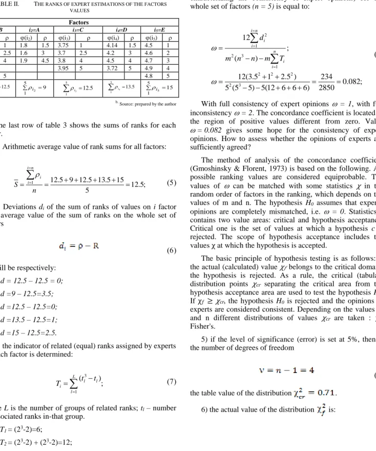
TABLE II. THE RANKS OF EXPERT ESTIMATIONS OF THE FACTORS VALUES Factors i1=B i2=A i3=C i4=D i5=E (i1) (i2) (i3) (i4) (i5) 1.2 1 1.8 1.5 3.75 1 4.14 1.5 4.5 1 1.4 2.5 1.6 3 3.7 2.5 4.2 3 4.6 2 1.12 4 1.9 4.5 3.8 4 4.5 4 4.7 3 3.95 5 3.72 5 4.9 4 1.1 5 4.8 5 5 1 5 . 12 1 i 5 1i2 9
5 1 5 . 12 3 i 5 1 5 . 13 4 i 5 1i5 15 b.Source: prepared by the author
The last row of table 3 shows the sums of ranks for each factor.
1) Arithmetic average value of rank sums for all factors:
12.5; 5 15 5 . 13 5 . 12 9 5 . 12 1
n S n i i i 2) Deviations diof the sum of ranks of values on i factor from average value of the sum of ranks on the whole set of factors will be respectively: i1,d = 12.5 – 12.5 = 0; i2,d =9 – 12.5=3.5; i3,d =12.5 – 12.5=0; i4,d =13.5 – 12.5=1; i5,d =15 – 12.5=2.5.
3) the indicator of related (equal) ranks assigned by experts for each factor is determined:
( ); 1 3
L l l l i t t T where L is the number of groups of related ranks; tl – number of associated ranks in-that group.
i1,T1 = (23-2)=6;
i2,T2 = (23-2) + (23-2)=12;
i3,T3 = (23-2)=6;
i4,T4 = (23-2)=6;
i5,T5 = 0.
The concordance coefficient (the main indicator characterizing the consistency of expert opinions) for the whole set of factors (n = 5) is equal to:
2 1 2 3 1 2 2 2 2 3 12 ; ( ) 12(3.5 1 2.5 ) 234 0.082; 5 (5 5) 5(12 6 6 6) 2850 i n i i n i i d m n n m T
With full consistency of expert opinions = 1, with full inconsistency = 2. The concordance coefficient is located in the region of positive values different from zero. Value
= 0.082 gives some hope for the consistency of expert opinions. How to assess whether the opinions of experts are sufficiently agreed?
The method of analysis of the concordance coefficient (Gmoshinsky & Florent, 1973) is based on the following. All possible ranking values are considered equiprobable. The values of can be matched with some statistics χ in the random order of factors in the ranking, which depends on the values of m and n. The hypothesis H0 assumes that experts' opinions are completely mismatched, i.e. = 0. Statistics χ contains two value areas: critical and hypothesis acceptance. Critical one is the set of values at which a hypothesis c is rejected. The scope of hypothesis acceptance includes the values χ at which the hypothesis is accepted.
The basic principle of hypothesis testing is as follows: if the actual (calculated) value χ𝑓 belongs to the critical domain,
the hypothesis is rejected. As a rule, the critical (tabular) distribution points χcr separating the critical area from the
hypothesis acceptance area are used to test the hypothesis H0. If χ𝑓≥ χcr, the hypothesis H0 is rejected and the opinions of
experts are considered consistent. Depending on the values m and n different distributions of values χcr are taken : χ2,
Fisher's.
5) if the level of significance (error) is set at 5%, then if the number of degrees of freedom
the table value of the distribution .
; 64 . 1 5 . 142 234 ) 6 6 6 12 ( 4 1 ) 1 5 ( 5 5 ) 5 . 2 1 5 . 3 ( 12 1 1 ) 1 ( 12 2 2 2 1 1 2 2
n i i i n i i i f T n n mn d Therefore, the actual value is significantly larger than the table one, i.e. 1.64>0.71. The hypothesis H0 assumes that experts’ opinions are completely mismatched, i.e. = 0 is rejected. This fact makes it possible to finally make sure that there is sufficient consistency of experts ' opinions on the totality of the factors under consideration.
7) Experts' activity coefficient cexp:
Since the experts provided their opinion for all factors without exception, their activity is high and corresponds to the maximum possible value for all factors cexp: = 1.
Similarly, statistical and heuristic indicators of experts' opinion consistency are calculated for the remaining evaluation factors for the first stage of the project and the remaining stages. To maintain the experimental integrity, the environment dynamics (N) is calculated as the arithmetic average of both integrated indicators (directly on the stage and on the works of the stage). For this example N = (3.13+3.23)/2.
The final risk-benefit ratio, determined on the basis of the environment volatility rate , is calculated by the formula:
K
(
N
)
(
K
(
R
)
/
5
)
N
where
K
(
R
)
– the maximum possible risk-benefit ratio accepted by the investor (reasonable risk) – equals 2 in this paper;N
is the volatility rate obtained as the arithmetic average as described above.III. CONCLUSION
The investment project is carried out in the external investment environment. The unpredictability of interaction between the environment and the project is a source of investor's risks. To identify it, the approach of determining the risk-benefit ratio through the volatility rate (dynamics) of the environment is proposed.
For the convenience of the study, the environment is decomposed into two spheres – macro environment and micro environment, and further study of the project is carried out in parallel at two levels.
Uniformity of classification of risk factors of microenvironment (a, b, c, d, e) and macro environment (A, B, C, D, E) grouped in five groups provides possibility for application of methods of expert survey and estimation at levels of both spheres: for work – at micro level, and on stages – at the macro level. An opportunity to compare their average estimates increases the accuracy of the study.
The method of assessing the values of risk factors for each stage of the project is used. It allows the forecaster, according to the survey, to rank the risk factors by increasing values, as well as to evaluate statistical and heuristic indicators of the degree of consistency of experts' opinions.
This approach is important and interesting as it is instrumental in calculating the costs of the investment project implementation, taking into account the risk.
References
[1] Beshelev, S. & Gurvich, F. (1980). Mathematical and statistical methods of expert assessments. M.: Statistics.
[2] Doroshenko M. (2019a). “Statistical approach to the determination of numerical values of risk-benefit ratio in investment processes.” Innovation management, entrepreneurship and sustainability (IMES 2019), 151-160.
[3] Doroshenko M. (2019b). “Determination of the environment volatility rate of the investment project.” Financial Economics, 5 Chapter. 4, 373-375.
[4] Ennuste, Yu (1989). Stochastic economic models of adaptive optimal planning and problems of their coordination. M.: Nauka.
[5] Ermolyev, Yu. & Yastremsky, A. (1979) Stochastic models and methods in economic planning. M.: Nauka.
[6] Gmoshinsky, V. & Fliorent, G. (1973). Theoretical foundations of engineering forecasting. M.: Nauka.
[7] Maksimov, Yu. (1983). “On some position of the theory of risk analysis.” Mathematical-stochastic methods in economic analysis and planning. Novosibirsk: Nauka.
[8] Mikhalevich, V. & Volkovich, V. (1983). Computational methods of research and design of complex systems. M.: Nauka.
[9] Moiseev, N. (1981). Mathematical problems of system analysis. M.: Nauka.
[10] Saati, T. (1993). Decision making. Method of analysis of hierarchies. M.: Radio and communications.
[11] Sokolov, V. & Smirnov, V. (1990). Study of flexibility and reliability of economic systems. Novosibirsk: Nauka.
[12] Vitlinsky, V. (1995). Risk is an economic category. From strategic planning to strategic management. Delovaya Ukraina, 40, 2.
[13] Vitlinsky, V. (1995). Risk modelling in transformation management. K.: KGEU.
[14] Yastremsky O. (1992). Modelling of economic risk. K.: Lybid. [15] Yudin, D. (1979). Tasks and methods of stochastic programming. M.: