Projecting input-output tables for model baselines

(1)

Projecting input-output tables for

model baselines

Temursho, U., Cardenete, M. A., Wojtowicz. K., Rey Los Santos, L., Weitzel, M., Vandyck, T., Saveyn, B.

2020

(2)

This publication is a Technical report by the Joint Research Centre (JRC), the European Commission’s science and knowledge service. It aims to provide evidence-based scientific support to the European policymaking process. The scientific output expressed does not imply a policy position of the European Commission. Neither the European Commission nor any person acting on behalf of the Commission is responsible for the use that might be made of this publication. For information on the methodology and quality underlying the data used in this publication for which the source is neither Eurostat nor other Commission services, users should contact the referenced source. The designations employed and the presentation of material on the maps do not imply the expression of any opinion whatsoever on the part of the European Union concerning the legal status of any country, territory, city or area or of its authorities, or concerning the delimitation of its frontiers or boundaries. Contact information

Name: Luis Rey Los Santos

Address: Joint Research Centre, Edificio Expo, Calle Inca Garcilaso, 3, 41092 Sevilla Email: [email protected] Tel.: +34 9544 88336 EU Science Hub https://ec.europa.eu/jrc JRC120513 EUR 30216 EN

PDF ISBN 978-92-76-18844-5 ISSN 1831-9424 doi:10.2760/5343

Luxembourg: Publications Office of the European Union, 2020 © European Union, 2020

The reuse policy of the European Commission is implemented by the Commission Decision 2011/833/EU of 12 December 2011 on the reuse of Commission documents (OJ L 330, 14.12.2011, p. 39). Except otherwise noted, the reuse of this document is authorised under the Creative Commons Attribution 4.0 International (CC BY 4.0) licence (https://creativecommons.org/licenses/by/4.0/). This means that reuse is allowed provided appropriate credit is given and any changes are indicated. For any use or reproduction of photos or other material that is not owned by the EU, permission must be sought directly from the copyright holders.

All content © European Union, 2020

How to cite this report: Temursho, U., Cardenete, M. A., Wojtowicz, K., Rey Los Santos, L., Weitzel, M., Vandyck, T. and Saveyn, B., Projecting input-output tables for model baselines, EUR 30216 EN, Publications Office of the European Union, Luxembourg, 2020, ISBN 978-92-76-18844-5, doi:10.2760/5343 JRC120513.

(3)

Acknowledgements

Authors

Umed Temursho, Manuel Alejandro Cardenete

Department of Economics, Loyola Universidad Andalucía, Campus Palmas Altas, C/ Energía Solar 1, Ed. G, 41014 Seville, Spain. E-mail: [email protected]

Krzysztof Wojtowicz, Luis Rey Los Santos, Matthias Weitzel, Toon Vandyck, Bert Saveyn European Commission - Joint Research Centre, Edificio Expo, Calle Inca Garcilaso, 3, 41092 Seville, Spain

(5)

Abstract

This technical report describes a multi-regional generalized RAS (MR-GRAS) procedure to update/project input-output tables or social accounting matrices. The method is able to incorporate a number of constraints on row and columns sums as well as specific flows between economic sectors and specific taxes in an input-output table. This feature is par-ticularly useful to reconcile information coming from different data sets. In the application described in this report, the method is tailored towards constraints with regard to the en-ergy system. Specifically, we specify constraints in the updating/projecting algorithm that are able to reproduce the economic values reflected in an energy balance from an energy system model. Here, we show that the method is able to generate input-output tables that are forward projected until 2050 and can be used as a baseline in a computable general equilibrium model like JRC-GEM-E3.

(6)

1 Introduction

Input-output tables (IOTs) or social accounting matrices (SAMs) serve as the data backbone of many economic models, in particular computable general equilibirum (CGE) models that take into account the dependencies between different sectors. In order to be used in such models, the data needs to be balanced. When building IOTs or SAMs from multiple data sources, these are usually inconsistent and require methods to balance them. In particular, this holds when IOTs or SAMs are updated to represent future years. In such way, they could be used as a baseline in CGE models (Wojtowicz et al., 2019). In this report, we describe a method that can be used to reconsile different data sources in the updating process of multi-regional IOTs or SAMs. In particular, we project tables through 2050, that can serve as input data to the JRC-GEM-E3 model.

The literature on updating, projecting, balancing and/or estimation methodologies of IOTs and/or SAMs is very extensive by now and is still growing. In fact, in general, it is impossible to considerall updating methods, because theoretically their number is infinite. To clarify this claim, consider a matrix estimation technique that is based on a linear or nonlinear programming approach with the aim of searching for the minimum distance between a given (i.e. available) original matrix and a new, to be estimated, matrix subject to certain constraints. It should not be surprising to realize that the definition of distance could be, in general, considered as a rather arbitrary or subjective concept, since poten-tially aninfinite number of functionscan be defined and adopted as a measure of distance of the two matrices. Nonetheless, there are a few updating methods that are (much) more popular among practitioners due to their certain attractive properties related to their the-oretical and practical considerations. Consequently, such updating/balancing methods are widely used by input-output economists, applied economic/environmental/energy/climate modellers who seriously consider the diverse (direct and indirect, price and quantity, etc.) mechanisms of intersectoral impacts, and by the statistical institutes around the world.

As a brief summary, the methods that were shown to be performing well in practice in-clude the so-called RAS method (see e.g. Bacharach, 1970; Leontief, 1941; Stone, 1961), the minimum sum of cross entropies (MSCE) approach (Golan et al., 1994; Golan and Vogel, 2000) and the matrix updating methods proposed by Harthoorn and van Dalen (1987) and Kuroda (1988). Other alternative approaches applied in practice are the Euro method (Beu-tel, 2002; Eurostat, 2008), the normalized squared differences method (Friedlander, 1961), the normalized absolute differences technique (Matuszewski et al., 1964), the squared dif-ferences approach (Almon, 1968), a univariate method of statistical correction (Tilanus, 1968), the so-called TAU and UAT methods of Snower (1990), maximum sum of cosine similarity indices (Cardenete and Sancho, 2004), mathematical programming approaches (see e.g. Canning and Wang, 2005; Harrigan and Buchanan, 1984) and more complex multi-objective optimization methods (see e.g. Strømman, 2009). Extensive empirical as-sessments of various (selected) matrix updating methods are carried out in Jackson and Murray (2004), Huang et al. (2008) and Temurshoev et al. (2011). The last two studies also include the improved versions of some of the above-mentioned methodologies, where improved refers to the treatment of negative elements and/or preservation of signs of the existing data points in the derived/projected tables.

The well-known RAS method arguably the most popular updating method, at least, among the practitioners from statistical agencies is a biproportional technique that is used to estimate a new matrix from an initial matrix by scaling its entries row- and column-wise so that the pre-specified, exogenously given row and column totals of the projection table are respected.1 _{However, the traditional RAS can only handle non-negative}

matri-ces, which limits its application to RASing non-negative matrices only. This is, indeed, a serious limitation in practice, in particular, when dealing with medium to large-scale IOTs, supply and use tables (SUTs) and SAMs (or, in general, any other matrix) as these often always include negative entries in such items (depending on the adopted table setting) as taxes net of subsidies, net exports, changes in inventories, trade and transportation mar-gins, and depreciation. Thus, the extension of RAS, called the generalized RAS (GRAS) method, originally proposed by Günlük-“enesen and Bates (1988), but re-discovered and more rigorously formalized by Junius and Oosterhaven (2003), is now a widely used bi-proportional technique for updating or balancing IOTs and/or SAMs with both positive and negative elements (see also Temurshoev et al., 2013). The SUT-RAS approach, proposed 1_{See Lahr and de Mesnard (2004) for details of the RAS method (including its history), which also gives an}

extensive set of references on the topic.

(7)

by Temurshoev and Timmer (2011), applies the GRAS updating idea for thejointestimation of supply and use tables for their different settings, such as the SUTs frameworks at basic prices and purchasers' prices, and a setting in which use tables are separated into domestic and imported use tables.2

In practice, as we have mentioned earlier, among the practitioners, in particular, national statistical offices, the (G)RAS approach is more popular, in our view, largely due to its simplicity and thus easier implementation (i.e. programming) requirements. Therefore, our choice here is a version of the GRAS method adopted to multi-regional IO setting. However, the MSCE approach could have been additionally adopted in certain cases when really complicated constraints needed to be imposed on the SAMs estimates that could not be easily incorporated within the GRAS setting in a transparent form. The next section, will briefly discusses the properties of these two updating methods in a comparative setting.

The rest of this report is organized as follows. In Section 2.1 the GRAS and MSCE approaches to updating IOTs/SAMs are presented and some of their properties discussed. Section 2.2 proposes the extension of the GRAS method, which we refer to as the multi-regional GRAS (MR-GRAS) approach, that additionally allows for imposition of aggregation constraints on the subsets of the IOT/SAM to be projected. The MR-GRAS technique is then used in our projections of the baseline SAMs for the years of 2015 to 2050 in five year steps. The details of these baseline projections are discussed in Section 3 and Section 4 concludes.

2_{The SUT-RAS method was/is used to construct the time-series of national SUTs, which are the building blocks}

(8)

2 Methodology for projecting/updating SAMs

2.1 Generalized RAS method vs. the minimum sum of cross

en-tropies (MSCE) approach

To fully understand the nature of the two mentioned updating methods, their mathematical formulations have to be first presented. Let x0

ij and xij be the ij-th element of the initial (available) and adjusted/projected (unknown before the projection) SAMs, respectively. Denote the known sum of row i's entries by ui = Pjxij, which, by SAM's construction, is also equal to the SAM column i's total, i.e. ui =Pkxki. Following Junius and Oosterhaven (2003), first define the ratio of the unknown (or new ) to the known (or old ) entries of SAM by zij ≡ xij/x0

ij whenever x0ij 6= 0. For x0ij = 0, this ratio should be set to unity, i.e. zij = 1(Lenzen et al., 2007). Then, the GRAS problem, used for a SAM

construction/updat-ing/projection purposes, has the following form:

min zij f(Z) =X i X j |x0ij|zijln zij e such that X j x0_ijzij =ui for alli= 1, . . . , n, X k x0_kjzkj=vj for allj= 1, . . . , n, (1) where |x0

ij| is the absolute value ofx0ij ande is the base of natural logarithm.3 Notice that for a SAM setting, it must always hold that vi = ui for all i. However, for the generality purposes here we still keep explicit the distinction between the row sumui and the column sum vi. In fact, even within the SAM setting the necessity (or possibility) of incorporating additional available information into the estimated SAMs may very well require the two sums to be entirely different, which is true for the current application.

The by now well-known solution of the GRAS problem Eq. (1) can be shown to be equal to xij = _r ix0ijsj forx0ij ≥0, r−_i 1x0 ijs −1 j forx 0 ij <0, (2) where ri > 0 and sj > 0 are, respectively, the row and column multipliers. In updating

input-output coefficients tables,ri andsj have clear economic interpretation: Stone (1961) termed the economic phenomena of uniform changes along any row as substitution ef-fects, while those of uniform changes down any column of the input coefficients matrix as fabrication effects. That is, the former refers to the substitution of one input for another throughout industrial processes, while fabrication effect refers to the changed proportion of value-added vs. intermediate inputs in a sector's total purchases.

From the GRAS optimal solution Eq. (2) it follows that ... the procedure RAS is appropri-ate for positive elements, but needs to be replaced by (1/R)A(1/S) for negative elements" (Günlük-“enesen and Bates, 1988, p. 476). The complete analytical expressions of the (unit-free) multipliers ri andsj are presented in Temurshoev et al. (2013), which are used in an iterative algorithm in order to obtain the projected (bi-proportionally adjusted) SAM. Thus, the existence of the closed-form solution makes GRASing a rather simple proce-dure to implement in practice, which moreover does not require advanced optimization and programming knowledge. Two other important (economic) structure-keeping properties of the GRAS method, as immediately seen from Eq. (2), are its sign-preservingand zero-preservingproperties. Thus, positive (negative) elements in the benchmark SAM keep their signs after projection procedure, while zero entries in the base-year SAM remain zeros in the adjusted SAM. The fourth crucial property of the GRAS method is that it doesnot make a difference for the final GRAS outcome whether the benchmark SAM (or IOT) is given in terms of absolute transactions values, input coefficients, or output coefficients (see Diet-zenbacher and Miller, 2009). This uniqueness property could be also considered as an 3_{Two notes are in place with respect to the form of the GRAS objective function. First, it is sometimes written}

without the base of the natural logarithm. This omission would not cause any problem and the two formulations would be entirely equivalent as long as the incorporated constraints fix the overall sum of the projected matrix elements, i.e. whenP

i,jxijis kept constant. Second, Huang et al. (2008) instead propose an Improved GRAS" function off1(Z) =Pi,j|x0ij|[zijln(zij/e) + 1]. However, one can easily observe that this adjustment does not play any role in determining the derived optimal solution, hence can be safely ignored.

(9)

important additional advantage of the GRAS approach, which is not shared by any other updating method.

Golan et al. (1994) use cross-entropy formulation to estimate the input coefficients of a SAM, defined as aij ≡xij/uj, such that the entropy distance between the estimated and base-year input coefficients are minimized. Thus, the minimum sum of cross entropies (MSCE) problem has the following mathematical optimization form:

min aij f(A) =X i X j aijln aij a0 ij ! such that X j

aijuj =ui for alli= 1, . . . , n, X

k

aki= 1and0≤aij≤1 for all i, j= 1, . . . , n,

(3)

where the benchmark input coefficient is defined asa0_ij ≡x0_ij/u0_j.

From the MSCE construction, it follows that the existence of negative elements in a SAM, which is to be updated or used for projection purposes, must be excluded. This is a rather serious limitation of the MSCE approach since negative transactions, as mentioned earlier, are always present in the reasonably dissaggregated real-world SAMs. An ad hoc and simple solution to dealing with this problem is to treat a negative expenditure as a positive receipt or a negative receipt as a positive expenditure. That is, if xij is negative, we simply set the entry to zero and add the value toxji. The `fipping' procedure will change row and column sums, but they will still be equal (Robinson et al., 2001, p. 49). This solution, however, is quite arbitrary as it might very well lead to an undesired significant (structural) change of the entire projected/updated SAM compared to its benchmark SAM. The solution of the MSCE problem Eq. (3) combines the information of the data and prior in an analogy to the Bayesian principle as follows:

aij = a0_ijexp (λiuj) P i P ja0ijexp (λiuj) .

That is, in Bayesian parlance, the posterior distribution (aij) equals to the product of the prior distribution (a0

ij) and the likelihood function (probability of drawing the data given parameters one is estimating), dividing by a normalization factor to convert relative prob-abilities into absolute ones. However, since the solution depends on Lagrangian multipli-ers (λi's) that cannot be determined by the problem's first-order conditions, there is no closed-form solution. Hence, it must be found numerically and often an efficient computing algorithm is used based on an unconstrained dual MSCE formulation (for details, see e.g. Golan and Vogel, 2000, pp. 451-453).4

On a theoretical note, McDougall (1999) makes a detailed comparison of RAS and other entropy-theoretic methods, including the MSCE technique, and argues that, in general, the RAS remains the preferable matrix balancing technique. In particular, he shows that compared to RAS, the MSCE revises cost structures more drastically for large industries than for small (Proposition 4, p. 9), which implies that the MSCE model tends to stay closer to the initial estimates for small industries (that is, for columns with small target totals), and to deviate from them more for large industries (large target totals) that in practice would seem rarely appropriate (p. 10). He also shows that the RAS preserves the ordering of input intensities across industries , while in general, the MSCE estimates do not preserve the intensity ordering (Proposition 5, p. 10). And it is also difficult to argue against the fact that the MSCE is less transparent than the RAS (p. 10). All and all, these and earlier mentioned properties of the GRAS method explain why this approach is chosen as our final preferred choice of the SAMs updating technique in this application.

In the literature some modifications of the traditional RAS method have been proposed that deal with the issue of accounting for additional available information on the projected 4_{Temurshoev (2012) applies minimum cross-entropy approach to the so-called} _{benchmarking problem}_{, also}

related to matrix updating, where the less precise high-frequency data are to be adjusted in order to match the more reliable low-frequency data. Morilla et al. (2005) and Cardenete and Sancho (2006) use the MSCE method to construct SAMs for Spain.

(10)

SAM. Consider a case when aset of transactions5 _{of the future SAMs are known, because,}

for example, the relevant entries need to be certain percentages higher or lower than the respective elements of the benchmark SAM or the baseline scenario's SAMs. Within the GRAS setting this is a rather straightforward modification.6 _{Let us denote by}_K _{the matrix}

of known elements of the future SAM X (thus the two have the same dimension). K has

zeros in all unknown entries of X that have to be estimated. Since the known entries do not have to be recovered, the corresponding elements in the benchmark SAM are nullified, resulting in an adjusted base-year SAM denoted asXe0. Next, the row totals ui and column totalsvi have to be modified as well, which might not be equal to each other if the changes to be made are asymmetric a more realistic picture of the available future information. In particular, the sum of all the relevant known elements has to be subtracted from the respective totals, i.e. the adjusted SAM's row totals and column totals are computed from e

ui = ui−Pjkij and evi = vi− P

jkji, respectively. Thus, the (G)RAS algorighm can now be implemented using the modified benchmark SAM Xe0, the adjusted row totalsui_e and the adjusted column totals_evi, and would give the updated SAM, denoted byXe. In the final step, the known information have to be incorporated into this matrix, i.e. the final SAM is then obtained asX=Xe+K. This modified GRAS procedure works because of its zero-preserving property.

Very often the required available information may take the form ofaggregates (sum) of

certain entries of SAM/IOT. An example of incorporating known information onaggregates

of submatrices of a larger matrix to be estimated can be considered the case of

updat-ing/projecting interregional IOT that necessarily has to be consistent with the available national IOT. Such traditional RAS extensions have been already proposed and assessed by Oosterhaven et al. (1986) and Gilchrist and St. Louis (1999, 2004). Whereas the first paper does not allow for overlapping aggregates of cells in the target table, such possibil-ity is allowed in the last two mentioned papers. Finally, the most flexible framework, the so-called KRAS (K for Konfliktfreies, i.e. free of conflicts), as proposed by Lenzen et al. (2009), generalizes the GRAS method to: (i) incorporate constraints on arbitrary subsets of matrix elements, including non-unity coefficients restrictions where the constraint co-efficients can be different from 1 or -1, (ii) include reliability of the initial estimate and the external constraints, and (iii) find a compromise solution between conflicting external information and inconsistent constraints. It is, however, not surprising that such flexibility comes at the expense of substantial programming and computational requirements, and thus the method becomes less transparent as any other complex numerical optimization technique, including the MSCE model with various extra, possibly conflicting, restrictions.

2.2 Multi-regional generalized RAS

In this section, we present an extension of the GRAS technique to a multi-regional IOT/SAM setting, which necessarily implies inclusion of additional aggregation constraints that make the disaggregated, inter- and intra-regional data consistent with the aggregated, national data. We refer to this extension as Multi-Regional Generalized RAS method, or simply as MR-GRAS approach. As mentioned in the last paragraph of Section 2.1, such extensions have been already made by Oosterhaven et al. (1986) , Gilchrist and St. Louis (1999, 2004) and Lenzen et al. (2009). However, while the first three studies focus on updating of non-negative matrices only, the last due to its generality in many respects loses the inherent transparency and simplicity properties of the GRAS approach. In particular, our contributions are as follows. First, we consider updating of a multi-regional IOT/SAM which allows for updating/projecting positive as well as negative entries. The inclusion of neg-ative entries into a multi-regional updating framework is clearly an important addition as there are more possibilities of having negative elements within a multi-regional IOT/SAM setting compared to a national one due to higher economic heterogeneity of regions (resp. countries) making up a whole economy (resp. economic area or the world). Second, we provide the complete analytical solution of the MR-GRAS approach, and derive an easy and 5_{These could be also input coefficients, not absolute values of the transactions, but as discussed earlier this}

distinction does not really matter within the GRAS framework.

6_{We do not discuss such extensions with the MSCE approach, as it is pretty clear that one will have to simply add}

any desired constraint to the basic MSCE problem Eq. (3) given that the solution will anyway have to be derived numerically. However, in order not to loose the transparency of the GRAS solution in terms of its closed-form expressions, it is always preferable that the relevant modifications are accounted for explicitly in its solution, if feasible.

(11)

simple iterative algorithm for its computation. There are several advantages of having such transparency:

No need for implementation and possessing the advanced knowledge of the more complex numerical optimization techniques.

No necessity of having access to a high-performance solvers, since the iterative ap-proach could be easily programmed/applied with such widely available software as Excel or R.

Easier control of the convergence process as compared to some built-in functions of the available optimization solvers. In particular, in cases of non-convergence one could derive the approximate solution simply by increasing only one threshold level used in the iterative approach. Then by studying the derived tables, especially the multipliers, one would be able to find the exact source of the non-convergence problem at lower threshold levels. In contrast, in solvers for such cases one usually has to change many stopping rule criteria which is often not straightforward, in particular, if the researcher has little knowledge of the complex algorithms underlying such optimization routines. And third, the adjustment multipliers used in MR-GRASing will have clear economic inter-pretations that could very well be the focus of research. These multipliers make up the MR-GRAS analytical solution and are thus directly accessible as the outputs of its itera-tive algorithm. In contrast, such information cannot be retrieved from the applications of numerical optimization techniques.

Using the notations as introduced in Section 2.1, the MR-GRAS problem for updating or projecting a benchmark multi-regional IOT/SAM, denoted by a rectangularm×nmatrixX0, is given by: min zij f(Z) =X i X j |x0_ij|zijln z_ij e such that X j x0_ijzij =ui for all i= 1, . . . , m, X k x0_kjzkj=vj for allj = 1, . . . , n, X i∈I,j∈J

x0_ijzij =wIJ for all I= 1, . . . , m0 < mandJ = 1, . . . , n0< n.

(4)

Compared to the GRAS problem Eq. (1), in the MR-GRAS problem Eq. (4) we have added the lastI×J aggregation constraints that ensure the consistency of the updated table entries with the exogenously given aggregated data. For simplicity of exposition, we have not added additional super(sub)scripts explicitly distinguishing between the disaggregated (i.e. intra- and inter-regional) variables and the aggregated (e.g. national) data.

To find the solution of Eq. (4), first, following Junius and Oosterhaven (2003), let us decompose the original matrix as X0 =P0−N0, where P0 contains the positive elements of X0, and N0 contains the absolute values of the negative elements of X0. Then the Lagrangean function of the MR-GRAS problem is

L= X (i,j)∈P0 x0_ijzijlnzij e − X (i,j)∈N0 x0_ijzijlnzij e +X i λiui−X j x0_ijzij +X j τjvj−X i x0_ijzkj+X (I,J) µIJwIJ− X i∈I,j∈J x0_ijzij,

whereλi,τj andµIJ are the Lagrange multipliers of the three respective sets of constraints in Eq. (4). The optimal solution of this function can be easily derived as:

xij = _tIJ_·_rix0 ijsj forx 0 ij ≥0, t−_IJ1·r_i−1x0 ijs −1 j forx0ij <0, (5) where ri ≡eλi _>₀, _sj _≡_eτj _>₀ and _tIJ _≡_eµIJ _>₀. Thus, as with the GRAS solution Eq. (2), the row and column multipliers are given by ri and sj, respectively. However, importantly

(12)

in contrast to the GRAS method, the MR-GRAS approach is no longer a bi-proportional technique as the aggregation multipliers tIJ's make its solution aggregation-specific for each aggregation sets of I andJ. Thus, not surprisingly with tIJ = 1 for allI and allJ, i.e. without aggregation constraints, the MR-GRAS solution boils down to that of the GRAS.

The benchmark IOT/SAM decomposition into its positive and negative parts, X0=P0−

N0, will be useful in finding the analytical expressions of the three sets of MR-GRAS multi-pliers. Given that its equivalent element-wise decomposition is x0_ij =p0_ij−n0_ij, the solution Eq. (5) can be also compactly written as:

xij =tIJ·rip0ijsj− 1 tIJ 1 rin 0 ij 1 sj. (6)

We do not provide here the mathematical details of the analytical expressions of the three multipliers and the proposed MR-GRAS iterative algorithm. For all these details, the interested reader is referred to Temursho et al. (2019).

(13)

3 Baseline projection of SAMs up to 2050

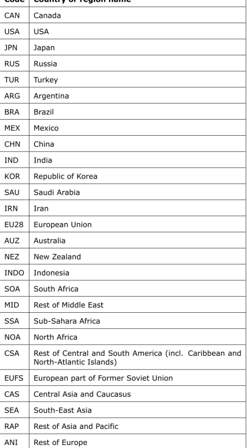
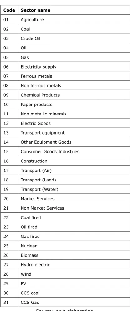
In this section, the details of SAMs projections are presented, starting with a (brief) dis-cussion of the exogenously given data that have to be imposed on the projected SAMs. The described updating steps completely match the MATLAB code structure as used for the projections purposes. The benchmark SAMs used in the projections come from the GTAP database version 9 (Aguiar et al., 2016) as employed in the JRC-GEM-E3 model (www.JRC-GEM-E3.net). The benchmark data include national SAMs for 27 regions, each covering 31 industries, and the respective bi-lateral trade data by sector, all for the year of 2011. The regional and industry classifications are given, respectively, in Table 2 and Table 3 in the Appendix. The aim is that the MR-GRAS projection produces the SAMs that are suitable as a baseline for JRC-GEM-E3, and that adhere to a number of exogenous constraints.

3.1 Baseline exogenous data

The task is projecting SAMs for eight projection years of 2015, 2020, 2025, 2030, 2035, 2040, 2045, and 2050. Hence, for all these years reasonably thought paths of exogenous variables are required that will ultimately drive the SAMs projection. The following data are exogeneously imposed on the projected SAMs, which for convenience we call thebasic overall structure constraints. In principle, all the technical work related to these pro-jections is carried out in MATLAB, but for further transparency purposes some of the data are also reported in the Excel file named Baseline .

1. Aggregate GDP values for all 27 regions and 8 projection years. These are derived by the Joint Research Centre (JRC) using the OECD's GDP growth rates and the 2011 GTAP9 relevant data.

2. Aggregate private consumption figures for all 27 regions and 8 projection years as percentages of GDP, that can for example represent an evolution of consumption shares following rising per capita income. In what follows, Con denotes (the vector of) private consumption values, disaggregated by sectors.

3. Aggregate government consumption figures for all 27 regions and 8 projection years as percentages of GDP. In what follows,Govdenotes (the vector of) government consumption values, disaggregated by sectors.

4. Sectoralinvestment(Inv) andcapital compensation(Cap) figures for all 27 regions and 8 projection years. These data are given exogenously primarily because they need to be in line with the (relevant block of the) JRC-GEM-E3 model, and as such are fully consistent with its dynamic modeling features.

5. Aggregate net exports or trade balance figures for all 27 regions and 8 projection years as percentages of GDP. In what follows, N etExp denotes (the vector of) net export values, disaggregated by sectors. Note that it must be the case that per region the following identity holds: GDPr=Ps(Con

r

s+Govrs+Invsr+N etExprs), whererrefers to a specific region andsto sectors.

6. Total demandor, equivalently,total supply(DemorSup) figuresby sectorfor all 27 regions and 8 projection years. For energy goods these figures are given exogenously (to be discussed below), while for non-energy goods the Demvalues were derived in the following three steps. First, sectoral private consumption, government consump-tion, and net exports were initially estimated by allocating their respective overall country-level values for all the projection years across sectors using their respective benchmark (2011) sectoral structures (i.e. shares by sector that sum to unity per these categories and per region). There is no need to do such preliminary estima-tions for investment vectors as another category of final demand, as these data are exogenously specified. Second, sectoral exports Exp are derived as a constant pro-portion (based on the benchmark data) of the net exports obtained in the first step. And finally, the Dem (equivalently, Sup) figures are obtained as the solution of the (single-country) open Leontief model corresponding to the vectors of thesum of the four obtained final demand categories (i.e. Con, Gov, Inv, andExp), where the 2011 input structures of all regions were used in all projections. The Leontief model allows

(14)

estimatingDem/Supfigures that fully (i.e. directly and indirectly) satisfy the total final demand figures estimated in the first two steps. Note that it would not make (much) sense to use the growth rates of the sum of the obtained final demand categories by sector in directly deriving the corresponding Dem data, since in general and also in our case there exist sectors without final products at all (e.g. Coal in many regions), hence one of the problems of applying final demand growth rates toDemseries. How-ever, what needs to be considered is that the outputs of such sectors (along with those of other sectors) are still used in the production process of the rest of sectors in the economy. Therefore, all these missing (indirect) interrelations are fully accounted for by using the Leontief model. As an outcome, the growth rates of Dem of the last 10 sectors (sectors 22 to 31), representing ten different technologies/inputs to electricity production, are exactly equal to the growth rates of the relevant Electricity supply sector (sector 06) simply because the output of these sectors is used only in the Elec-tricity supply sector. It is important to note that the separate vectors of final demand categories and net exports as obtained in the above-mentioned steps are not taken as the final projections of these variables, but are used solely for the purposes of estimatingreasonable sector-specific growth ratesof total demand/supply.

7. The sum of gross value added (GVA) and taxes less subsidies (TxS) by sector,

which for simplicity we denote asTotGVA_TxS. The projections of TotGVA_TxS were

obtained in two steps. First, the Dem growth rates were applied to the benchmark TotGVA_TxS figures in order to obtain the initialTotGVA_TxS estimates. In the second

step, per region these initial TotGVA_TxS's by sector were adjusted (often upwards)

such that their sum matches the exogenously specified GDP values (which corresponds to the income-side GDP measurement, and is generally not guaranteed in the first step). However, not all sectoral figures were allowed to be adjusted because such adjustments of small data could lead to a negative intermediate demand (i.e. the difference Dem−TotGVA_TxS should be non-negative). After many experiments, we

ended up with an admittedly somewhat ad-hoc rule of allowing adjustingT otGV A_T xS figures of only those sectors whose private consumption is at least 0.6% of the total private consumption per region.

8. Sectoral shares of high- and low-skilled labor and of crude oil reservesfor all 27 regions and 8 projection years, provided by JRC.

Besides the above basic overall structure constraints, also certain sector or product-specific constraints are imposed. In particular, additionally energy products/sectors-specific constraints are imposed, which are compactly given in an MRIO format within the MATLAB file named EnergyTab . These energy sectors are Coal (sector 02), Crude oil (sector 03), Oil (sector 04), Gas (sector 05), Electricity supply (sector 06), and sectors 22 to 31 representing different technologies of electricity production (e.g. Coal fired, Oil fired, Nuclear, Biomass, etc.). The energy-specific constraints include:

9. Domestic supply of energy goods, which is defined as total intermediate demand plus gross value added.

10. Trade data, both exports and imports, distinguished by origin and destination. 11. All items of taxes (i.e. VAT, subsidies, indirect taxes, and duties).

12. Imports' transportation margins.

13. Private consumption and government consumption.

14. Individual (cell-specific) intermediate uses: crude oil uses in the oil sector (potentially fixed), the uses of coal, oil and gas by sectors Ferrous metals and Non metallic minerals , and the uses of different technologies (sectors 22 to 31) in electricity supply sector.

All these individual energy sectors projections are based on energy balances derived from the energy model POLES-JRC.

Finally, once considering the economy-environment interactions we need to account for emissions-related constraints/data. These include:

(15)

15. The value of CO₂ tax by sector (potentially) for all 27 regions and 8 projection years. These taxes are related to CO₂ emissions from combustion of fossil fuels, and in what follows are denoted byTaxCO2.

16. The value of other greenhouse gasses related with the output (production activi-ty/level) of all sectors, (potentially) for all 27 regions and 8 projection years. These include CO2emissions from industrial processes, CH4, N2O, HFCs, etc. In what follows

the related taxes are termed GHG taxes and denoted asTaxGHG.

All the emissions-related data are again fully consistent with the projections of the POLES-JRC model.

3.2 Projection steps description

The main philosophy of our projection approach is to have the maximum possible direct control over the updating process. This implies that the practice of full automatization of the wholeSAM/IOT projection very often could lead to inferior results, as also our own ex-perience shows. Instead, all the existing information for the framework at hand has to be fully utilized (which often differ from database to database), while additional objectives/as-sumptions of the baseline or simulation projections have to be respected. An example of the last requirement in our application is the requirement of having the identical taxes and subsidies rates by sector for the baseline projections.

The fact that sectoral trade data between all 27 regions (except for energy sectors as described above) have to be also estimated, the best way to proceed is using a (sort of) multi-regional input-output framework in the process of projections of the relevant parts of SAMs/IOTs. This is especially true because of the nature of the GTAP data in that it does not represent the detailed sectoral trade of intermediates and final goods separately as is always the case within a full-fledged multi-regional input-output setting.7 _{Given the}

importance of using a multi-regional input-output (MRIO) setting in the projections, we first present this setting relevant for the current project, which additionally provides a compact, macro overview of the global SAM/IOT.

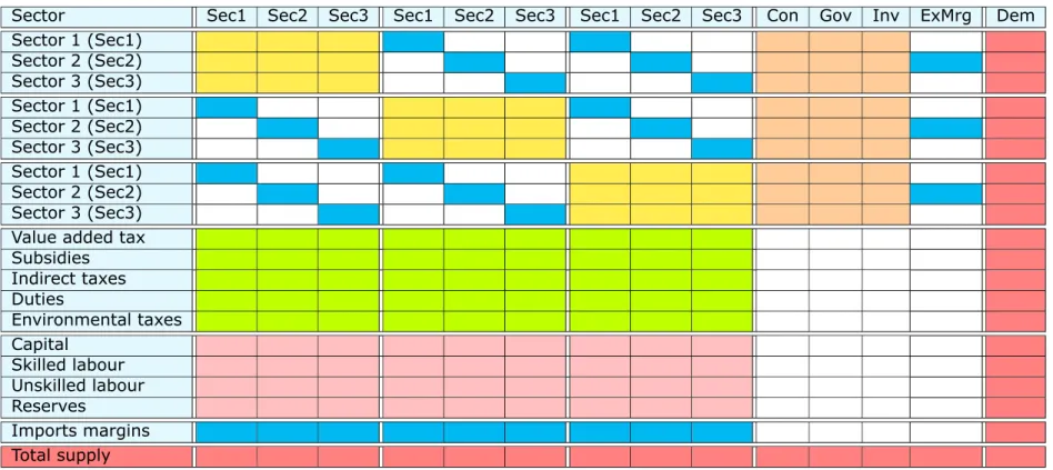
Table 1 illustrates the basic structure of an MRIO framework of the world economy, which for simplicity is assumed to consist of only 3 regions and 3 sectors. It should be noted that it is not a fully-fledged multi-regional input-output table since domestic intermediate uses are not separated from the imported uses of intermediate goods, and the trade data do not distinguish between trade in intermediates and in final goods. This feature of the GTAP database is, however, sufficient for CGE modeling purposes. Given this characteristics of the input data, the trade data have been included along the diagonal elements of the off-diagonal block-matrices of the MRIO inter-sectoral transactions table. All the trade data are illustrated in cyan in Table 1, which also includes the margins related to imports and exports (positioned, respectively, in the penultimate row and penultimate column). This again has to do with a specific way of treating international transportation margins in the GTAP model, which allows individual countries to export international transportation services to a global transport sector which subsequently satisfies demand for bilateral margins. Since only sector 2 is assumed to be a transport sector, only sector 2 can export transportation services. The sum of the imports margins exactly coincide with the total exports margins at the global level, but not (necessarily) at the levels of individual regions. Along the diagonal blocks of the MRIO table, the yellow blocks represent the total (i.e. domestic and imported) uses of intermediates by domestic sectors along the columns. Finally, the final demand categories (except for exports which are, by definition, part of the trade data) are given in orange, the gross value added (GVA) section in pink, and the taxes and subsidies (TxS) section in lime. The red margins are known exogenous data, corresponding to Dem (=Sup)figures and the global sum of GVA, TxS and final demand components. Uncolored

parts of the table refer to empty cells.

The procedure of projecting SAMs is implemented in two steps, which are described in what follows.

7_{Our expectations in this respect were confirmed during the initial stages of this project by pursing other two}

bottom-up approaches of SAMs projections, where first the national SAMs were projected for each region in two steps, and in the final stage the bilateral trade by sector were projected based on the obtained total export and total imports data from the previous steps. However, such attempts were unsuccessful (i.e. the final stage ended up to be a RAS-infeasible problem) basically due to having a sparse trade matrix.

(16)

Table 1: A hypothetical 3-region and 3-sector global (multi-regional) SAM/IOT

Sector Sec1 Sec2 Sec3 Sec1 Sec2 Sec3 Sec1 Sec2 Sec3 Con Gov Inv ExMrg Dem

Sector 1 (Sec1) Sector 2 (Sec2) Sector 3 (Sec3) Sector 1 (Sec1) Sector 2 (Sec2) Sector 3 (Sec3) Sector 1 (Sec1) Sector 2 (Sec2) Sector 3 (Sec3) Value added tax Subsidies Indirect taxes Duties Environmental taxes Capital Skilled labour Unskilled labour Reserves Imports margins Total supply

Note: The abbreviations Con, Gov, Inv, ExMrg and Dem denote, respectively, private consumption, government consumption, investment,

exports margins (i.e. exports of transportation services), and total demand. It is assumed that only sector 2 is a transport sector. Along the diagonal blocks of the multi-regional intersectoral flows table, the yellow blocks represent the total (i.e. domestic and imported) uses of intermediates by domestic sectors. The diagonal entries within the off-diagonal blocks of this matrix represent trade of both intermediate and final goods among the regions and are given in cyan; transport margins on imported goods and exported transportation services are also colored in cyan as these also make part of the trade data. Final demand categories (except for exports) are given in orange, GVA section in pink, and taxes and subsidies section in lime. The red margins are known exogenous data. Uncolored (white) cells indicate empty cells.

Source: own elaboration.

(17)

Step 1: Projection of all MRIO components, excluding those of GVA and TxS. This step is implemented using the MR-GRAS method discussed in Section 2.2, which allows for imposing aggregation constraints on private consumption and government consump-tion (corresponding to, respectively, points 2 and 3 in Secconsump-tion 3.1), and on intermediate demands of energy and non-energy sectors as certain intermediate demand components are also exogenously specified. The constraints on total intermediate demands of energy goods are derived as follows: first, total GVA of energy goods (TotGVA_energy) are obtained

as the difference between the corresponding known TotGVA_TxS figures and the relevant

energy-specific and emissions-related data on all taxes (corresponding, respectively, to points 7 and 11, 15 and 16 in Section 3.1); and, second, by subtracting TotGVA_energy

from the domestic supply of energy products (corresponding to point 10 in Section 3.1) we obtain the total value of intermediate demand to be imposed on energy sectors.

Thus, at this stage we impose 459 (= 27× 17) aggregation constraints on the

(above-mentioned) two categories of final demand and 15 total intermediate demands of energy sectors for all 27 regions, which are indicated as wIJ's in the MR-GRAS problem Eq. (4). Note that since investment vectors are exogenously given (see point 4 in Section 3.1), these are not projected within the MR-GRAS framework and are subtracted from the relevant total demand Dem figures. Additionally, the sectoral row sum restrictions (i.e. ui's in the MR-GRAS problem Eq. (4)) need to account for (i.e. subtract from the last differences Dem−

Inv) the row sums of the fixed elements representing the energy-specific constraints. This adjustment is necessary because in the projections the fixed elements are nullified within the reference structure matrix and are added later to the main MRIO structure, following themodified GRAS approachas fully explained in Section 1. On the other hand, the column sums for sectors, denoted asvj's in Eq. (4), are given by the differencesDem−TotGVA_TxS (see points 6 and 7 in Section 3.1) that are further adjusted by the column-sums of the fixed data related to the energy-specific constraints. The same adjustments need to be done with respect to all the aggregation constraints as well.

Finally, to ensure that the total transportation margins on imports and the exports trans-portation margins at the world level match each other, we: (1) add a negative element (equal to the sum of the benchmark-year exports margins which is, by definition, also equal to the global sum of imports margins in the benchmark table) in the last row and last column of the MRIO table to be projected, corresponding to the crossing-point of these international trade-related transportation margins, (2) set their corresponding row sum to zero, which will give the estimate of the global import transportation margins of non-energy sectors, and (3) set the sum of the exports margin column to the total of the exogenously given imports margins of the energy sectors (corresponding to point 12 in Section 3.1). It is not difficult to confirm that the last constraint ensures that the global export margins are equal to the sum of the global import margins of non-energy goods and those of energy goods.

Once we impose all the above-mentioned constraints, the trade balance restrictions will be automatically satisfied. That is, the net exports restrictions (point 5 in Section 3.1) are, in fact, redundant within the MRIO setting projections. This is a sort of Walras' Law, which within the MRIO setting is confirmed by the expenditure-side approach to GDP measure-ment stating that GDP equals the sum of private consumption, government consumption, investments, and net exports. As the MR-IOT/SAM is a closed system at the global level, the net exports are projected endogenously and must match the exogenously given figures as long as all the relevant imposed restrictions satisfy the expenditure-side GDP constraint and there are no exogenously imposed inconsistencies between the overall basic structure constraints and the individual sector-specific constraints. For example, the value on to-tal intermediate demand constraints on energy sectors adjusted for the sum of their fixed components cannot be negative by definition, while if there are positive cells to be en-dogenously estimated within the projection procedure along the energy sectors' columns, then the corresponding adjusted intermediate demand totals must be strictly positive. The same logical requirement applies to the adjusted totals of the final demand categories. All these checks are included in the MATLAB program as well, including the check on equality of exogenous regional net exports with their corresponding values endogenously derived within the MR-GRAS procedure.

With respect to the question of constraints consistency, we would like to emphasize the following. Given that the energy-specific and emissions-related constraints come from a completely different modeling approach (i.e. the POLES-JRC model), it is of crucial impor-tance that their consistency with the relevant national aggregation constraints be checked.

(18)

For example, given that the trade data of energy sectors are obtained from the POLES-JRC energy model, one has to make sure that per region the projections of net exports of en-ergy goods do not contradict the national net exports projections and the structure of net exports of non-energy sectors taken together.

Step 2: Projection of the components of TxS and GVA. We first discuss an allocation procedure related to the taxes on CO2 emissions from combustion of fossil fuels, TaxCO2.

From the emission-related data (see point 15 in Section 3.1), TaxCO2 is only given for fuel producers, which include three sectors of Coal (sector 01), Oil (04) and Gas (05). Although such representation is fine for the aims of the JRC-GEM-E3 model, for the purposes of presenting the final data in the format of input-output tables it is better to allocate the carbon taxes across all sectors using the mentioned fuels in the production process. The uses of fuels by all sectors are available from the MR-GRAS procedure of the previous step, whose values also include TaxCO2. For each year, each country and each fuel, we

simply allocate the corresponding total carbon tax revenues according to the shares of the used fuel in total fuel use by all sectors. Hence, the vector TaxCO2 has now values not only for fuel producers, but for all fuel users. These taxes are then subtracted from the intermediate uses of all the users of the fuel in question (which thus now do not include carbon taxes), and positioned instead as the carbon taxes component of all the taxesTxS.

It should be noted that the total demand figures for fuel-sectors should afterwards be adjusted downward equal to the size of carbon taxes of the fuel in question (not of all fuel sectors), since now TaxCO2 is allocated across all fuel users (and not concentrated only in the fuel producer sectors).

The above-mentioned procedure at first sight might seem a bit ad-hoc, but it is not. Assume that the total carbon tax on coal combustion is denoted by TaxCO2c. Further denote the carbon emission factor of coal by emf_c, the user price of coal by puc, the price of (one tonne of) CO2 emissions by pco2, and the value of the total use of coal by sectori

asuci. Given that (within the JRC-GEM-E3/POLES-JRC models) per fuel, per region and per year, the carbon prices, the user prices of fuel, and the emission factors are the same for all fuel-using sectors, then for each region and each year, sector i's carbon tax on its coal use can be more neatly determined as follows:

TaxCO2ci=pco2×emfc uci puc

(7) However, this is exactly how the sectoral carbon taxes were derived above, since the used allocation procedure boils down to Eq. (7):

uci P kuck ×TotCO2c= uci P kuck ×X k pco2×emfc uck puc =TaxCO2ci.

One of the requirements of this application is to have constant sector-specific rates of taxes and subsidies over time for the baseline projections for all non-energy sectors (recall from the energy-specific constraints that the relevant data are already exogenous for energy sectors). The components of TxS thus have to respect the relevant benchmark

rates, which imply the following formulas:

VAT = VATrate

1 +VATrate ×Con=VATcoef ×Con, (8)

Sub=SubRate×(IntDem+TotGVA), (9) InT ax=InT xRate×(IntDem+TotGVA+Imp−Exp−ExM rg), (10)

Duty=X r Dutyr= X r DutyRate_r× Impr 1 +SubRater+GHGrater , (11)

TaxGHG=GHGrate×(IntDem+TotGVA), (12) where all the overlined terms refer to the base-year constant rates, and the following ab-breviations are used: VAT = value added tax,Con= private consumption,Sub= subsidies, IntDem = total intermediate demand, TotGVA= total GVA (excluding TxS), Imp_r = total

imports from the import partner r, Imp = total imports (i.e. Imp = P

rImpr), InT ax = indirect taxes, Exp = total exports,ExM rg = exports of international transportation mar-gins, Dutyr = duties on imports obtained from the import partner (region)r, andGHGrate

(19)

is the tax rate of other GHG emissions. Notice that subsidies and GHG taxes are derived in the same way, using the same base of domestic supply. However, the difference is that while subsidies rates are kept constant, while the GHG tax rates are endogenously derived (using equation 12) in order to allow direct incorporation of the GHG tax revenuesT axGHG that are exogenously specified for all the projection years (see point in 16 in Section 3.1). Therefore, all other rates are readily computed using the 2011 benchmark data and the relevant formulas given in Eq. (8) Eq. (12). Also note from Eq. (11) that the base of duties are imports in volumes as specified in the JRC-GEM-E3 model, where the prices of imports besides domestic prices also account for subsidies and GHG emissions taxes of the exporting regions.

Eq. (8) implies that the value added tax (VAT) is straightforward to compute for all the

projection years, sinceConis already known from the first step discussed above. However, given that sectoral totals of GVA excluding taxes (TotGVA) are still unknown at this point,

one cannot use Eq. (9) Eq. (12) to obtain the values of subsidies, indirect taxes and duties. There is, however, a rather simple trick: use the input-side balance of the MRIO setting which states that for each sector the following identity should hold:

Sup=IntDem+Imp+ImM rg+TotTxS+TotGVA, (13) where ImM rg stands for imports international transportation margins, and total taxes is, by definition, given by TotTxS =VAT+Sub+IndT ax+Duty+TaxCO2+TaxGHG.

For the simplicity of the followup expressions, let us first introduce the following short-cut vector notations:

SR≡1 +SubRate, (14)

ITR≡1 +InT xRate, (15)

SITR≡1 +SubRate+InT xRate, (16)

DIM ≡DutyRate·IMP, (17)

F ≡Dem−

SITR·IntDem+ITR·Imp+ImM rg+VAT +TaxCO2+TaxGHG−InT xRate·(Exp+ExM rg)

, (18)

where IMP is the import (or trade) matrix consisting ofImp_r of all regions (thus excludes

international transportation margins) and has the MRIO setting format as described/illus-trated in Table 1 above,DutyRateis the matrix of the same structure asIMP but includes the

benchmark rates of duties, and·denotes element-wise multiplication (Hadamard product).

Then it can be easily shown that equations Eq. (9) Eq. (18) jointly imply the following system of two (vector) equations:

TotGVA=SITR\−1(F−Duty), (19)

Duty=DIM0 SRc+TaxGHG\

\

IntDem+TotGVA\ −1−1

, (20)

where x_brefers to a diagonal matrix with the elements of vector xalong its main diagonal and zero otherwise and a prime (0_{) denotes matrix transposition. Notice that equation Eq.} (20) is nothing else as the definition of duties in Eq. (11) written in a compact matrix form (using also the GHG taxes equation Eq. (12) in place of the GHG tax rates). In our MATLAB program, equations Eq. (19) and Eq. (20) are used within a loop format until the values of TotGVA converge for each projection year.8 Once TotGVA is obtained, the remaining

tax-related variables (i.e. subsidies, indirect taxes, duties, and GHG tax rates) are then straightforward to compute using their definitional equations.

Thus, for all the projection years and for all non-energy goods, the taxes and subsidy rates (except for GHG tax rates) are exactly equal to their benchmark-year counterpart rates. If there is a need to change (some of) these rates, the respective 2011 benchmark rates have to be exogenously adjusted. For transparency, the endogenously derived GHG rates are presented in Table 4 in the Appendix. It can be seen from the table that these 8_{This is the simplest (and possibly most understandable) way of solving Eq. (19) and Eq. (20) for}_TotGVA_;

furthermore, the convergence speed is very fast (for any positive initial/starting values of TotGVA) requiring

maximum up to 5 iterations for a very fine threshold level of 1.e-07. One, of course, can also substitute Eq. (20) in Eq. (19) and derive the correspondingmatrix quadratic equation. This could then be readily solved using the relevant solution involving the use of eigenvectors and eigenvalues, which is arguably a somewhat more complicated approach.

(20)

rates are rather stable over the projection years: the average annual change of the GHG rates (that are expressed in percentages) for the five countries/regions currently having positive GHG taxes (i.e. CAN, MEX, AUZ, CAS and ANI) is only -0.035%. In addition, we generally observe a negative trend in the GHG rates over time for all the regions involved, except for ANI (Rest of Europe) region where this trend is positive.

The components ofTotGVA for non-energy sectors are computed as follows. First, from TotGVA we subtract the exogenously given capital compensation (Cap) data (see point 4 in Section 3.1). The obtained difference,TotGVA−Cap, is then allocated across the remaining categories of GVA (i.e. high- and low-skilled labor and oil reserves) using their exogenously specified sectoral shares (see point 7 in Section 3.1).

The final projected SAMs/IOTs are made available in two Excel files, named Baseline projections_ MRIOs andBaseline projections_ NIOTs. The first presents the overall results within a global MRIO setting, similar in structure to that illustrated in Table 1, for each projection year. The second file presents the projections per country or region within a national input-output table (NIOT) setting. The last also includes the detailed sectoral exports and imports data by all trade partners.

3.3 Build-in checks

Part of the projections quality checks include the following:

1. the identity of the income-side GDP and the expenditure-side GDP by region, 2. aggregation constraints on private consumption by region,

3. aggregation constraints on government consumption by region, 4. aggregation constraints on investments by region,

5. aggregation constraints on each component of taxes and subsidies per region, 6. energy products/sectors-specific constraints, and

7. emissions-related constraints.

All these restrictions will be, by construction, satisfied as long as the derivation of the (modified) MR-GRAS solution is feasible at a low, acceptable convergence level. In this respect, we did not encounter any problem in projecting SAMs for the eight projection years. Moreover, additional checks on feasibility of imposing different constraints and on the correctness of the projection outcomes are already incorporated and explained within the MATLAB program, which are also (briefly) discussed in the previous section.

Zooming in further into the projection results requires an application of some sort of matrix distance" indicator that measures the closeness of one projected SAM/IOT to its benchmark structure/table or to that of another projected SAM/IOT. We use the following two closeness statistics, also widely used in the related literature (see e.g., Temurshoev et al., 2011):

1. Mean absolute percentage error, defined as:

MAPE = 1 N m X i=1 n X j=1 |xij−xbij| |xb ij| ×100,

where xb_ij is the benchmark element, xij is its estimate (or its counterpart projected element into the future), andN is the number of non-zero elements in the benchmark table. Forxb_ij = 0the corresponding difference is set to zero (as zero is preserved in all

the estimates anyhow), and note that the denominator is also taken in absolute value as this does not allow a reduction in the actual distance/error whenxb

ij <0. Therefore, MAPE shows the average percentage by which each projected element is either larger or smaller than its benchmark value, where all the relative percentage deviations are givenequal weightsof 1/N.

2. Weighted absolute percentage error, defined as:

(21)

which weights each percentage deviation of xij from xb

ij by the relative size of the cor-responding benchmark element in the overall sum of the benchmark elements (again taken in absolute values which ensures that the weights sum up to one). In other words, compared to MAPE, the WAPE statistics gives larger weight to the larger benchmark val-ues. Therefore, if WAPE is found to be smaller than the corresponding MAPE, then one can assert that, on average, the projection of larger values involves smaller errors than those of the small elements projection.

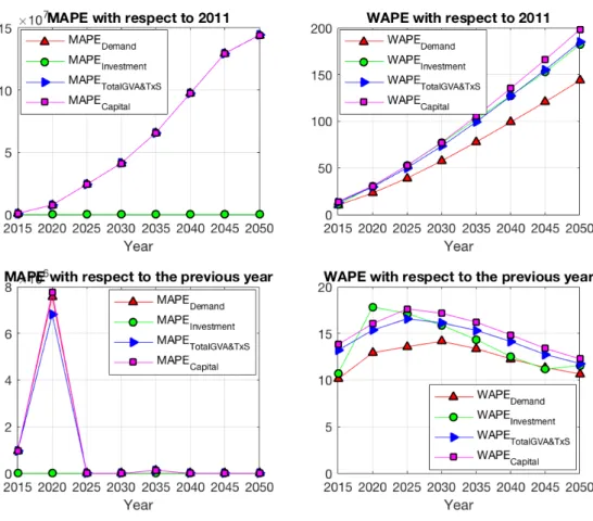
We start with the discussion of the closeness statistics of the exogenously given data points, which include total demand/supply, investment, the overall sum of GVA and TxS (TotGVA_TxS) and capital compensation data. In a sense it is clear that these data together

with the benchmark 2011 SAM/IOT structure determine the development over time and thus the overall performance/distances of our projections. Therefore, it is important to see how the MAPE and WAPE indicators behave for the exogenous data. These are illustrated in Figure 1. Not surprisingly, the MAPEs and WAPEs with the benchmark from the 2011 SAM/IOT show increasing trend over time, which fully represents the imposed exogenous (system-wide growth) assumptions. MAPEs and WAPEs with respect to the previous-period projection data as a comparison base, on the other hand, as illustrated in the bottom subplots of Figure 1, show rather stable distances (for MAPEs from 2020 and onward). Notice the very large percentage deviations for MAPEs both given with respect to the 2011 benchmark data and with respect to the previous year data. This is due to the fact that there are very small figures present in the data and their changes are individually large percentage-wise, but in general these are relatively so small numbers that could be safely disregarded. MAPE for investment is much lower than those of the rest simply because it has no such small figures. Note that these are anyway exogenously given deviations and have nothing to do with the projection procedure performance. This explanation of large MAPE deviations is exactly taken into account in WAPEs which show far much lower deviations. In particular, it shows that the system-wide exogenous period-to-period average increase in the entire MRIO data, which takes into account the size of each transaction, in the range of 10 to 15% is imposed.

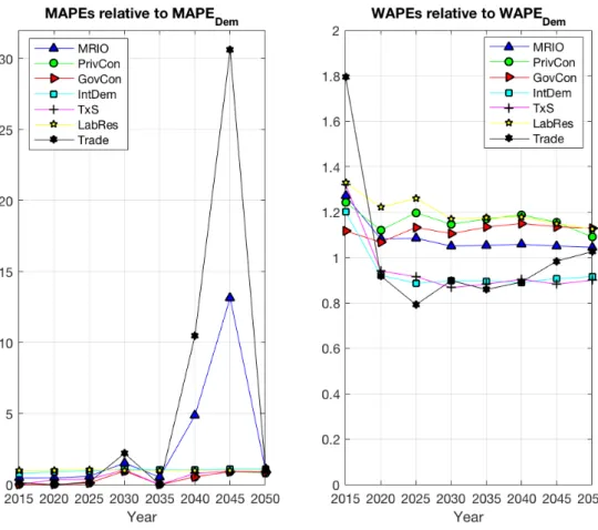
We computed the closeness statics of the seven sub-parts of the projected SAMs/IOTs: the entire MRIO table (MRIO), private consumption (Con), government consumption (Gov), intermediate demand matrices (IntDem), taxes and subsidies (TxS), high- and low-skilled

labor and oil reserves (LabRes), and the trade matrix (T rade). In Figure 2 these obtained MAPEs/WAPEs are presented relative to the corresponding MAPEs/WAPEs of total demand/-supply (Dem) for the purposes of taking explicitly into account the distances/errors intro-duced exogenously. In general, all the resulting relative MAPEs and WAPEs are satisfactory: they are close to unity, and the deviations are close to those of total demand. In fact, from Figure 1 we observe that the MAPEs/WAPEs of total demand are the lowest average ex-ogenous deviations allowed, because capital compensation data show the largest average exogenous deviations. Therefore, if we would have taken these last as the reference data for evaluating the performance of our projections, the distance indicators would have been lower. Additionally, it should be noted that some parts of the transactions related to energy sectors that were kept fixed in MR-GRAS procedure also exogenously contribute to these aggregate deviations.

We, however, observe oneunacceptabledeviation in MAPE comparing the 2045 to 2040 projections. The overall MRIO relative MAPE of 13 can be seen to be explained by the relative MAPE of the trade data which equals 30.6. That is, compared to the 2045-2040 MAPE of total demand, the relevant MAPE of trade data is 30 times larger. A closer look into the detailed deviations matrix of the corresponding trade data reveals the culprit: it is related to the imports of Electricity supply (sector 06) from all countries by New Zeland (NEZ). For example, the relevant import figure from the European part of Former Soviet Union region (EUFS) was only 0.000496 mln USD in 2040, but increased to 1.5386 mln USD by 2045 representing a dramatic increase of 310396%. Large deviations of similar magnitudes are observed for all other imports data of New Zeland. These deviations, however, have nothing to do with the MR-GRAS performance as the trade of energy goods are given exogenously in the form of energy-specific constraints (see point 10 in Section 3). In later versions of the MR-GRAS methodology, this is addressed by nulling specific trade flows for electricity that cannot be observed in the real world. This example shows the usefulness of MAPE indicators in revealing rather unrealistic changes in small transactions. This is exactly the reason why we prefer to use both MAPE and WAPE indicators in assessing

(22)

Figure 1: MAPE and WAPE of the exogenously given data matrix deviations.

3.4 Further updates to the methodology

While projecting IOTs/SAMs to build a baseline with the methodology described above, certain issues have arisen as is often the case in data-building practice, which led us to update or change the relevant parts of the procedure. Two adjustments are related to the projection of total demand (Dem) figures (hence we have updated the procedure discussed as point 6 in Section 3.1).

The first improvement in projecting total supply or total demand (Dem) series was im-posing a more reasonable assumption that all sectors (producing tradable goods) in each region contribute positively to the exogeneously imposed evolution of (i.e. change in) the aggregate net exports of the region. For example, if in region r aggregate net exports is increasing, then we add to the existing net exports figure ofeachtradable sector a compo-nent that is proportional to and consistent in sign (in the assumed case, positive) with the imposed aggregate change in net exports as follows:

N etExprs(t) =N etExprs(t−1) +ShareNX r s×

N etExpr(t)−N etExpr(t−1), (21) where N etExpr_s(t) is the net exports of sector s in region r in projection year t (note that these are not final estimates of sectoral net exports, but are only used for Dem projection purposes),N etExpr(t)is the aggregate net exports of regionrin yeart(this is exogenously specified data), and ShareNXrs is the relevant proportionality factor (or net exports "share ) for tradable sectors in regionr that is defined in terms of the benchmark-year net exports data (expressed in absolute value) as:

ShareNXr_s= |N etExp r s(t0)| P s|N etExprs(t0)| .

Next, we also use the structure of intermediate input purchases in the projection of Dem. The output-side balance states that total demand consists of intermediate and final

(23)

Figure 2: MAPEs/WAPEs relative to those of total demand/supply demands:

Dem=IntDem+Con+Gov+Inv+Exp. (22) Since we already have projections for private consumption Con, government consumption Gov and investments Inv, we need to have the preliminary projections of intermediate output IntDemand exportsExp. The last is obtained using net exports estimates from Eq. (21) asExp=N etExp+Imp, where total importsImp are defined in terms of the base-year imports coefficients, Imp =_bam×Dem. Finally, the intermediate outputs are derived using the intermediate input structure of the base year asIntDem=Aint×Dem. Thus, substituting these last variables in Eq. (22) and solving for total demand gives:

Dem= I−Aint−bam −1

Con+Gov+Inv+N etExp

. (23)

Equation Eq. (23) has been used to derive total demand (total supply) projections using the preliminary estimates of sector-specificCon, Gov,Inv andN etExpdata.

(24)

4 Conclusions

This paper describes a multi-regional generalized RAS methods designed to update/project input-output tables. In particular, the method is able to update/project tables taking into account various constraints on column and/or row sums as well as specific flows between sectors. The method is transparent in that the algorithm of computing the updated/pro-jected IOT/SAM can be derived in an explicit formulation. Furthermore, we are transparent in another dimension by making available the MATLAB code in the Appendix of this report. The underlying data structure for this particular application of the MR-GRAS methodology is tailored towards the JRC-GEM-E3 CGE model, e.g. with respect to the sectoral and regional aggregation of the tables and the structure of taxes and subsidies of the model. However, with the available code and the general formulation of the method, it could be easily adjusted towards other models or used for other purposes.

The constraints imposed on the updating/projection process are putting special emphasis on energy use and greenhouse gas emissions. The MR-GRAS method presented here is therefore capable of integrating detailed energy data (from different exogenous sources) into economic structure during the updating/projecting process. This can be of relevance to reconcile economic structure with energy statistics for a given year to derive a base year IOT/SAM, or as in this application a series of IOTs/SAMs going forward in time such that they can be readily used in a CGE model like JRC-GEM-E3. The constraint system available with the MR-GRAS methodology can for example be used to build economic tables that are fully consistent with exogenous energy balances.

In this report, several economic and energy constraints were assumed to be exogenous. The methodological framework employed at the JRC formulating these constraints and projecting IOTs/SAMs with the MR-GRAS method is referred to as PIRAMID (Platform to Integrate, Reconcile and Align Model-based Input-output Data) (Wojtowicz et al., 2019). The MR-GRAS methodology described in this report forms a crucial centrepiece of this PIRAMID framework, which has already successfully been applied in generating a baseline for model simulations with the JRC-GEM-E3 model. Further, such baseline tables generated with PIRAMID/MR-GRAS have been published (Rey Los Santos et al., 2018). This framework is continuously developed further to allow for better representation of energy flows and other aspects of projecting. The latest version of baseline generation software employed at the JRC might therefore differ from the code reproduced in the Appendix of this report.