Version December Add-on Module ALUMINIUM. Ultimate Limit State and Serviceability Limit State Design according to Eurocode 9

Add-on Module

ALUMINIUM

Ultimate Limit State and

Serviceability Limit State Design

according to Eurocode 9

Program Description

Version

December 2011

All rights, including those of the translation, are reserved. No portion of this book may be reproduced – mechanically, electronically, or by any other means, including photocopying – without written permission of ING.SOFTWARE DLUBAL.

© Ing. Software Dlubal

Am Zellweg 2 D-93464 Tiefenbach

Tel: +49 (0) 9673 9203-0 Fax: +49 (0) 9673 9203-51 E-mail: [email protected]

Contents

Contents Page Contents Page

1. Introduction 4

1.1 Add-on Module ALUMINIUM 4

1.2 ALUMINIUM Team 5

1.3 Using the Manual 5

1.4 Starting ALUMINIUM 6

2. Input Data 8

2.1 General Data 8

2.1.1 Ultimate Limit State 8

2.1.2 Serviceability Limit State 10

2.1.3 National Annex (NA) 11

2.2 Materials 12

2.3 Cross-Sections 14

2.4 Lateral Intermediate Supports 17

2.5 Effective Lengths - Members 18

2.6 Effective Lengths - Sets of Members 22

2.7 Nodal Supports - Sets of Members 23

2.8 Member Releases - Sets of Members 25

2.9 Serviceability Data 26

3. Calculation 27

3.1 Details 27

3.1.1 Ultimate Limit State 27

3.1.2 Stability 28

3.1.3 Serviceability 30

3.1.4 Other 31

3.2 Start Calculation 32

4. Results 34

4.1 Design by Load Case 34

4.2 Design by Cross-Section 35

4.3 Design by Set of Members 36

4.4 Design by Member 36

4.5 Design by x-Location 37

4.6 Governing Internal Forces by Member 38

4.7 GoverningInternalForcesbySetof

Members 39

4.8 Member Slendernesses 39

4.9 Parts List by Member 40

4.10 Parts List by Set of Members 41

5. Evaluation of Results 42 5.1 Results on RSTAB Model 43

5.2 Result Diagrams 45

5.3 Filtering Results 46

6. Printout 48

6.1 Printout Report 48

6.2 Print ALUMINIUM Graphics 48

7. General Functions 50 7.1 ALUMINIUM Design Cases 50

7.2 Cross-Section Optimization 52

7.3 Import and Export of Materials 54

7.4 Units and Decimal Places 55

7.5 Export of Results 55

8. Example 57

A Literature 69

1.

Introduction

1.1

Add-on Module ALUMINIUM

Eurocode 9 determines rules for the design, analysis and construction of aluminium struc-tures in all member states of the European Union. With the add-on module ALUMINIUM from the company ING.SOFTWARE DLUBAL all users obtain a highly efficient and universal tool to design aluminium structures according to this standard. The rules specific for particular countries are set in national annexes. In ALUMINIUM a great number of national annexes is already available. It is also possible for the user to define limit values and create new na-tional annexes in the module.

All typical designs of load capacity, stability and deformation are carried out in the module ALUMINIUM. Different actions are taken into account during the load capacity design and there is the possibility to choose some interaction designs for a given standard. The alloca-tion of designed cross-secalloca-tions into classes 1 to 4 makes an important part of the design according to Eurocode 9. The purpose of this classification is to determine the range in which the local buckling in cross-section parts limits the load capacity so that the rotational capacity of cross-sections can be verified. Further, ALUMINIUM automatically calculates the c/t ratios of compressed parts and carries out the classification automatically.

For the stability design, you can determine for every single member or set of members whether buckling is possible in the direction of y-axis and/or z-axis. Lateral supports can be added for a realistic representation of the structural model. All comparative slendernesses and critical loads are automatically determined by ALUMINIUM on the basis of the bounda-ry conditions. For the design of lateral torsional buckling, the elastic critical moment that is necessary for the design is calculated automatically. It can also be entered manually. The lo-cation where the loads are applied, which influences the elastic critical moment, can also be defined in the detailed settings.

The serviceability limit state has become important in modern civil engineering as more and more slender cross-sections are being used. In ALUMINIUM, load cases and groups and combinations of load cases can be arranged individually to cover the various design situa-tions.

Like other modules, ALUMINIUM is fully integrated into the RSTAB program. However, it is not only an optical part of the program. Results from the module can be incorporated to the central printout report. Therefore, the entire design can be easily – and uniformly – or-ganized and presented.

The program includes an automatic cross-section optimization and a possibility to export all modified profiles to RSTAB.

Individual design cases make it possible to flexibly analyze separate parts of extensive struc-tures.

We wish you much success and delight when working with our module ALUMINIUM. Your ING.SOFTWARE DLUBAL company.

1.2

ALUMINIUM Team

The following people participated in the development of the ALUMINIUM module:

Program Coordinators

Dipl.-Ing. Georg Dlubal Ing. Ph.D. Martin Čudejko

Dipl.-Ing. (FH) Younes El Frem Ing. Pavol Červeňák

Programmers

Ing. Zdeněk Kosáček

Ing. Ph.D. Martin Čudejko Zbyněk Zámečník

Dr.-Ing. Jaroslav Lain

Ing. Martin Budáč Mgr. Petr Oulehle Ing. Roman Svoboda DiS. Jiří Šmerák

Library of Cross-Sections and Materials

Ing. Ph.D. Jan Rybín Jan Brnušák

Design of Program, Dialog Boxes and Icons

Dipl.-Ing. Georg Dlubal MgA. Robert Kolouch

Ing. Jan Miléř

Testing and Technical Support

Ing. Ctirad Martinec Ing. Ph.D. Martin Čudejko Dipl.-Ing. (FH) Steffen Clauß Dipl.-Ing. (FH) Matthias Entenmann Dipl.-Ing. (FH) René Flori

Dipl.-Ing. (FH) Walter Fröhlich Dipl.-Ing. (BA) Andreas Niemeier Dipl.-Ing. (FH) Walter Rustler M. Sc. Dipl.-Ing. (FH) Frank Sonntag Dipl.-Ing. (FH) Christian Stautner

Manuals, Documentation and Translations

Ing. Ph.D. Martin Čudejko Ing. Ladislav Kábrt Ing. Mgr. Hana Macková Ing. Petr Míchal

Mgr. Michaela Kryšková Mgr. Petra Pokorná Dipl.-Ing. (FH) Robert Vogl Dipl.-Ü. Gundel Pietzcker

1.3

Using the Manual

All general topics such as installation, user interface, results evaluation and printout report are described in detail in the manual of the main program RSTAB. Hence, we omit them in this manual and will focus on typical features of the add-on module ALUMINIUM.

During the description of ALUMINIUM, we use the sequence and structure of the different input and output tables. We feature the described icons (buttons) in square brackets, e.g. [Pick]. The buttons are simultaneously displayed on the left margin. The names of dialog boxes, tables and particular menus are marked in italics in the text so that they can be easily found in the program.

1.4

Starting ALUMINIUM

It is possible to initialize the add-on module ALUMINIUM in several ways.

Main Menu

You can call up ALUMINIUM by the command from the main menu of the RSTAB program:

Additional Modules →Design - Aluminium→ALUMINIUM.

Figure 1.1: Main Menu: Additional Modules→Design - Aluminium→ALUMINIUM

Navigator

Further, it is possible to start ALUMINIUM from the Data navigator by clicking on the item

Additional Modules → ALUMINIUM.

Panel

If results of ALUMINIUM are already available in the RSTAB position, you can set the rele-vant design case of this module in the list of load cases in the menu bar. The design criteri-on criteri-on members is displayed graphically in the work window of RSTAB by using the [Results on/off] button.

The [ALUMINIUM] button that enables you to start of ALUMINIUM is available in the panel.

Figure 1.3: [ALUMINIUM] button in Panel

2.

Input Data

The data of the design cases is entered in different tables of this module. Furthermore, the graphic input using the function [Pick] is available for members and sets of members. After the initialization of the ALUMINIUM module, a new window is displayed. In its left part, a navigator is shown that enables you to access all existing tables. The roll-out list of all possibly entered design cases is located above this navigator (see chapter 7.1, page 50). If ALUMINIUM is called up for the first time in a position of RSTAB, the following important data is loaded automatically:

• Members and sets of members

• Load cases, load groups and load combinations

• Materials

• Cross-sections

• Internal forces (in the background – if calculated)

You can switch among the tables either by clicking on individual navigator items of ALU-MINIUM or by using the buttons visible on the left. The [F2] and [F3] function keys can also be used to browse the tables in both directions.

Save entered data by the [OK] button and close the module ALUMINIUM, while by the

[Cancel] button you terminate the module without saving the data.

2.1

General Data

In the table 1.1 General Data, members, sets of members and actions are to be selected for the design. You can specify load cases, groups and combinations for the ultimate limit state and the serviceability limit state design separately in the corresponding tabs.

2.1.1

Ultimate Limit State

Design of

You can select both Members and Sets of Members for the design. If only specific objects are to be designed, it is necessary to clear the check box All. By doing so, both input boxes become accessible and you can enter the numbers of the relevant members or sets of mem-bers there. With the [Pick] button, you can also select memmem-bers or sets of memmem-bers graph-ically in the RSTAB work window. To rewrite the list of default member numbers, select it by double-clicking it, and then enter the relevant numbers.

If no sets of members were defined in RSTAB yet, they can be created in ALUMINIUM via the [New Set of Members…] button. The familiar RSTAB dialog box to create a new set of members opens in which you enter the relevant data.

Designing a set of members has the advantage that the total maxima of the design ratios is determined of all members contained in the set. In this case, the results tables 2.3 Design by Sets of Members, 3.2 Governing Internal Forces by Set of Members and 4.2 Parts List by Set of Members are displayed additionally.

National Annex (NA)

This list box controls the national annex which is to be applied for the design parameters and limit deformations.

Use the [Edit] button open a dialog box in which you can check or modify the settings of the selected national annex. This dialog box is explained in chapter 2.1.3 on page 11.

Existing Load Cases / Load Groups and Load Combinations

All design-relevant load cases, load groups and load combinations that were created in RSTAB are listed in these two sections. The [] button moves the selected load cases, load groups or load combinations to the list Selected for Design on the right. Single items can be also transferred by double-clicks. The [] button moves all items to the list on the right. If an asterisk (*) is displayed at load cases or combinations, as you can see e.g. in Figure 2.1 at load cases 8 to 10, they are excluded from the design. It signifies that no loads were as-signed to these load cases or that they contain only imperfections (as in our example). Please note that only load combinations can be chosen whose minimum and maximum val-ues can be determined unambiguously (i.e. alternative combinations with the combination criterion Permanent). This restriction is necessary because the calculation of the elastic criti-cal moment at lateral buckling requires the unambiguous assignment of moment diagrams. If an invalid load combination is selected, the following warning appears:

Figure 2.2: Warning when selecting invalidLC, LG or CO

A multiple choice of load cases can be done by using the [Ctrl] key, as a routine procedure in Windows. Hence, you can select and transfer several load cases to the list on the right simultaneously.

Selected for Design

The loads selected for the design are listed in the right column. By the [] button you can remove the selected load cases, load groups or combinations from the list. As before, they can be transferred by double-clicks. The [] button removes all items from the list.

Generally, the calculation of an enveloping Or load combination is faster than the analysis of all contained load cases or groups. On the other hand, you must keep in mind the above-mentioned restriction: to determine the maximum or minimum values unambiguously, the Or load combination must only contain load cases, groups or combinations which enter the combination with the criterion Permanent. Moreover, the design of an enveloping load combination makes it a bit difficult to retrace the influence of the contained actions.

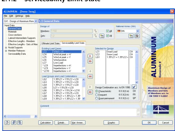
2.1.2

Serviceability Limit State

Figure 2.3: Table 1.1 General Data, Serviceability Limit State tab

Existing Load Cases / Load Groups and Load Combinations

All load cases, load groups and load combinations that were created in RSTAB are listed in these two sections.

Selected for Design

Adding load cases and their groups and combinations to the list for the design, resp. re-moving them from the list is done in the same way like in the previous tab (see chapter 2.1.1).

Design Combination acc. to EN 1990

In this dialog section, you can set different limit values that are to be applied for the deflec-tions of combined acdeflec-tions.

The relevant limit value for the selected design combination can be assigned as follows: Click the action in the list Selected for Design to select it. Then click the the blue tick [] to allocate the relevant criteria. The limit values are controlled by the National Annex. They they can be modified in the dialog box that contains the parameters of the national annex (see Figure 2.4, page 11).

The governing reference lengths for the SLS design are managed in table 2.9 (see chapter 2.9, page 26).

Comment

In this entry field you can make a comment on the current case in ALUMINIUM.

The [Nat. Annex] button enables you to open the dialog box any time to check or modify the following parameters of the current National Annex: partial safety factors, limit values for SLS design and limit ratio for general yield criterion (see chapter 2.1.3).

2.1.3

National Annex (NA)

In this list, the National Annex can be selected whose design parameters and limit defor-mation values are to be applied.

Use the [Edit] button to open the dialog box with detailed settings of the selected National Annex (see Figure 2.4). You can also modify some parameters, if necessary.

By the [New] button, it is possible to create a user-defined national annex.

The buttons located in the left bottom corner enable you to save the modified parameters as default or, by contrast, to restore the default settings of the program.

Any user-defined National Annex can be removed by using the [Delete] button.

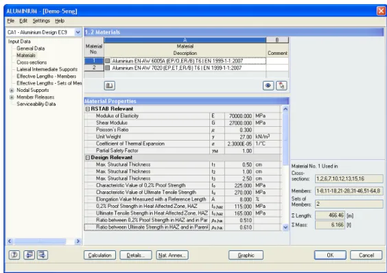
2.2

Materials

This table is divided into two parts. The materials for the design are listed in the upper part. In the lower part, the Material Properties of the current material are displayed, i.e. the ma-terial whose line is selected in the upper table.

Materials that are not used for the design are written in gray letters. Inadmissible materials are displayed with red, modified materials with blue fonts.

The material properties that are necessary to calculate the internal forces in RSTAB are de-scribed in detail in the RSTAB manual, chapter 5.2. The design-relevant material characteris-tics are stored in the global material library. Those are automatically set as default.

Units and decimal places of the material properties and stresses can be edited from the main menu Options→ Units and Decimal Places (see chapter 7.4, page 55).

Figure 2.5: Table 1.2 Materials

Material Description

The materials that have been defined in RSTAB are set by default. You can also enter mate-rials manually here. If the Material Description corresponds to an entry in the material li-brary, ALUMINIUM automatically imports the relevant material properties.

To select a material from the list, place the cursor in column A and click on the [] button or press the [F7] function key. A list is opened that you can see on the left. As soon as you have chosen the appropriate material, the material characteristics are updated in the table below.

This list of materials includes only materials from the category Aluminium. How to import materials from the library is described below.

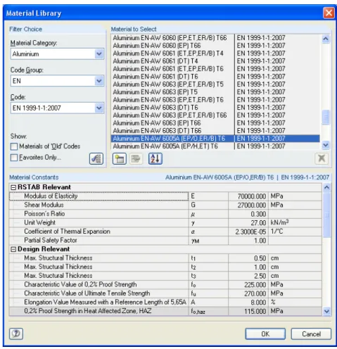
Import Material from Library

A considerable amount of materials is stored in the library. Open the library via menu

Edit → Material Library…

or by clicking on the button visible on the left.

Figure 2.6: Material Library dialog box

In the section Filter Choice, the material category Aluminium is set by default. In the list Ma-terial to Select which is located on the right, you can select a particular maMa-terial, and in the lower part of the dialog box you can check its characteristic values. After clicking on [OK] or pressing the [↵] key, the material is taken over to the table 1.2 of ALUMINIUM.

Chapter 5.2 of the RSTAB manual explains in detail how materials can be filtered, added to the library or newly classified.

Only materials included in EN 1999-1-1 (table 3.2) are supported in ALUMINIUM. Further-more, it is not possible to modify the material properties in the add-on module.

ALUMINIUM does not check the product form of the material (see [1] Table 3.2b, column Product form) and the shape of the cross-section. Thus, the appropriate material has to be selected by the user.

General cross-sections (shaded)

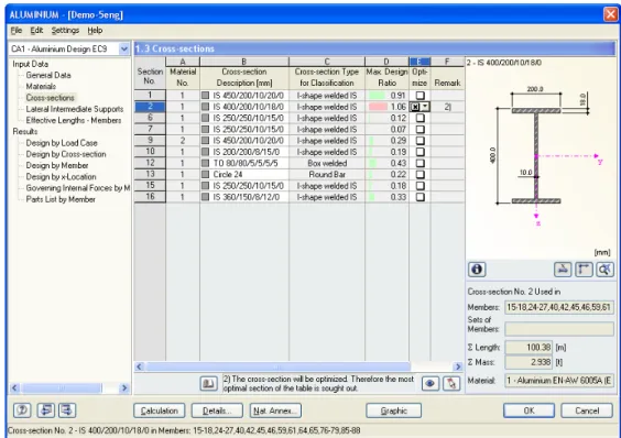
2.3

Cross-Sections

This table controls the cross-sections that are to be designed. The parameters for the opti-mization can be defined here as well.

Figure 2.7: Table 1.3 Cross-sections

Cross-Section Description

When you open this table, the sections that were defined in RSTAB are set by default, in-cluding the assigned material numbers.

The cross-sections can be changed any time for the design. The description of a modified cross-section is highlighted in blue color.

In order to edit a cross-section, enter the new description in the corresponding line or select the new section from the library. Open this library as in RSTAB by clicking on the [Import Cross-Section from Library…] button. Alternatively, place the cursor in the corresponding line and click on the [...] button or press the [F7] key. The RSTAB library resp. the dialog box with the cross-section table of the input line opens.

Chapter 5.3 of the RSTAB manual describes in detail how cross-sections can be selected from the library.

ALUMINIUM allows for the comprehensive design of the following types:

• I sections: rolled/welded, doubly symmetrical or symmetrical about z-axis only

• Hollow and box sections: rolled/welded, square or rectangular, doubly symmetrical

• Solid sections: round and flat bars

• Pipes

• Angles: rolled/welded single sections with equal or unequal legs

• T sections: rolled/welded, symmetrical about z-axis

• Channels: rolled/welded, symmetrical about y-axis

It is also possible to design other cross-sections of the RSTAB library or SHAPE-THIN which are labeled as "General". For those, some specific features of design are not available, how-ever. SHAPE-THIN sections must have straight elements exclusively in order to be designed.

Figure 2.8: Cross-Section Library

Tapered Member

It is not possible to design tapered members in ALUMINIUM. This type of combined cross-sections is not supported. There will be error 1021) after the calculation.

Info about Cross-Section

There are different display options for stress points and c/t cross-section parts: Select the cross-section in table 1.3 and open the following dialog box by clicking the [Info] button.

The currently selected cross-section is displayed in the right part of the dialog box. The vari-ous buttons below have the following functions:

Table. 2.1: Buttons for Cross-Section Graphics

Max. Design Ratio

This column is only displayed after the calculation. Due to those values, you can decide whether to carry out an optimization. It is apparent from the design ratios and colored rela-tion scales which cross-secrela-tions have a low utilizarela-tion and therefore are oversized, resp. which sections are overstrained and too weak.

Optimize

Every cross-section of the library can be optimized. During the optimization process, the cross-section within the same table of cross-sections is determined on the basis of the in-ternal forces from RSTAB which fulfills best the maximum design ratio.

The maximum allowable design ratio for the optimization is controlled in the Details dialog box (see Figure 3.4, page 31). Further information on the optimization of cross-sections can be found in chapter 7.2 on page 52.

Remark

In this column, the references to footnotes (below the list of cross-sections) are shown. If the message Incorrect cross-section data! is shown, then this is due to a cross-section that is not contained in the cross-section library. It may be a user-defined cross-section or a sec-tion that was not calculated in the module SHAPE-THIN. Via the [...] button in column B Cross-section Description, you can set a cross-section that is suitable for the design (see Figure 2.8).

There are several Welded Cross-sections in the section library. Those are parameterized sec-tions that are usually combined by welding sheets in steelwork. Please note that the design of welds (effect of HAZ) is not implemented in the current ALUMINIUM program version.

Button Function

The stress points are switched on and off.

The cross-section parts (c/t) are switched on and off.

The numbering of stress points, resp. of cross-section parts (c/t) is switched on and off.

The details of stress points, resp. of cross-section parts (c/t) are displayed. The dimensioning of the cross-section is switched on and off.

The principal axes of the cross-section are switched on and off.

2.4

Lateral Intermediate Supports

In this table, lateral intermediate supports on members can be defined. The program always assumes these supports as perpendicular to the minor axis z (see Figure 2.9) of the cross-section. Hence, it is possible to change the effective lengths of the member that are im-portant for the design of buckling and lateral torsional buckling.

Lateral intermediate supports are always considered as forked supports for the design.

Figure 2.10: Table 1.4 Lateral Intermediate Supports

In the upper part of this table, up to nine lateral intermediate supports can be created per member.The lower part of the table displays the summary of the entered data for the mem-ber that is selected in the upper table.

Lateral intermediate supports can be defined either by directly entering the distances or by specifying the support locations Relatively. For the latter, it is necessary to tick the associat-ed check box below the list. The relative distances of the supports are then calculatassociat-ed from the member lengths.

If the Member-like Input (see dialog box Details, Stability tab as displayed in Figure 3.2, page 28) is used for straight sets of members, lateral supports can be applied to the inter-mediate nodes of each set of members. If not, it is not possible to place lateral supports di-rectly in nodes.

2.5

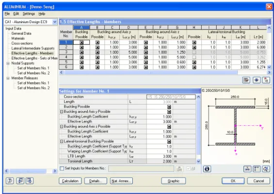
Effective Lengths - Members

The table 1.5 consists of two parts so that a good overview of the data is given. In the up-per table, the buckling length coefficients kcr,y and kcr,z, the effective lengths Lcr,y and Lcr,z, the lateral-torsional buckling coefficients kz and kw and the effective lengths Lw and LT are sum-marized for every member. In the lower part of this table, detailed information on the member that is selected in the upper table is displayed.

Figure 2.11: Table 1.5 Effective Lengths - Members

The effective lengths for the buckling about the minor principal axis are automatically aligned with the input in the previous table 1.4. If a member is divided into different lengths by lateral intermediate supports, then no values are displayed in the corresponding columns G, K and L of the table 1.5.

It is possible to change the buckling length coefficients both in the summary table in the upper part and in the detailed settings in the lower part. The data of the corrresponding part of this table is then updated automatically. The buckling length of a member can also be defined graphically by using the function [Pick].

The tree structure in the lower part of the Settings for Member table contains the following parameters:

• Cross-section

• Length (actual length of the member)

• Buckling Possible (cf. column A)

• Buckling around Axis y (buckling lengths, cf. columns B to D)

• Buckling around Axis z (buckling lengths, cf. columns E to G)

• Lateral-torsional Buckling Possible (lateral-torsional buckling length coefficient and lengths, cf. columns H to L)

It is also possible to modify the Buckling Length Coefficients in the relevant directions and decide whether the buckling design is to be executed. If the buckling length coefficient is changed, the respective effective member length is modified automatically.

If the option Lateral-torsional Buckling Possible is unchecked, there is no design of lateral torsional buckling due to bending about the major axis. Torsional buckling and torsional-flexural buckling due to axial compression are automatically disabled, too.

Buckling Possible

For the stability design of the buckling and lateral buckling, it is necessary for the member to transfer compression forces. Members that cannot transfer compression forces due to their definitions (e.g. tension members, elastic foundations, rigid couplings) are a priori ex-cluded from the stability design in ALUMINIUM. Those lines are grayed out and a corre-sponding comment is displayed in the column Comment.

The column Buckling Possible enables you to classify specific members as compression ones or, alternatively, to exclude them from the design. Hence, the check boxes in column A and also in table Settings for Member No. control whether the input options for the buckling length parameters are accessible for a member.

Buckling around Axis y / Axis z

The columns Possible control if a member is to be designed for buckling around its axes y and/or z. The axis y represents the "major" principal member axis, the axis z the "minor" principal member axis. The buckling length coefficients (effective length factors) kcr,y and kcr,z can be freely chosen for the buckling around the major and minor axes.

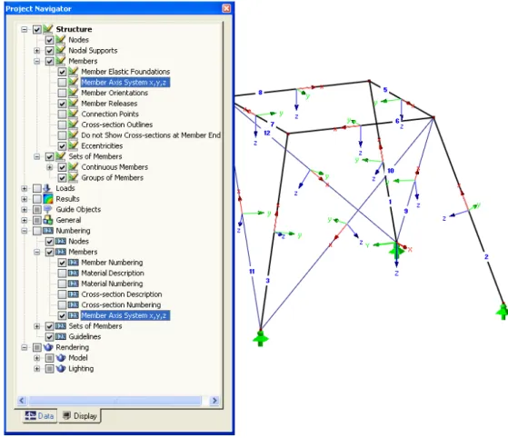
The orientation of the member axes can be checked in the cross-section graphics of the ta-ble 1.3 Cross-Sections (see Figure 2.7). In the RSTAB work window which can be opened any time via the [Graphic] button, you can display the local member axes from the Display navigator.

If buckling is possible around one or both member axes, the precise values can be entered in columns C and D respectively F and G or in table Settings for Member No. below. If you define the buckling length coefficient kcr, the buckling length Lcr is determined by multiplying the member length L with this buckling length coefficient. The input fields are interactive.

Via the [...] button at the end of the Lcr input fields, you can select two nodes in the RSTAB

work window graphically. Their distance then defines the buckling length.

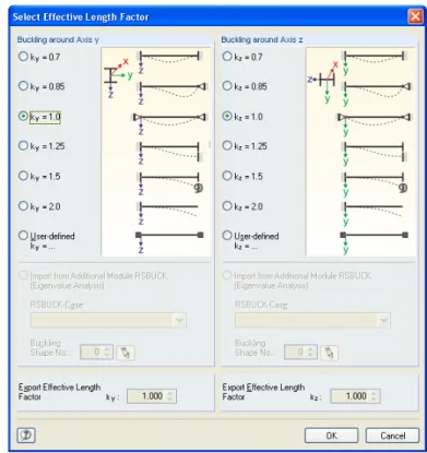
The effective length factors of the members can also be defined in a special dialog box which is called by the button [Select Effective Length Factor] below the upper table.

Figure 2.13: Dialog box Select Effective Length Factor

The predefined values of effective length factors k_cr,y and k_cr,z correspond to the following definitions in [1], Table 6.8:

k= 0.70 held in position at both ends + restrained in direction at both ends k= 0.85 held in position at both ends + restrained in direction at one end k= 1.00 held in position at both ends + not restrained in direction at either end k= 1.25 held in position at one end + restrained in direction at both ends

k= 1.50 held in position and restrained in direction at one end + not held in position and partially restrained in direction at other end

k= 2.00 held in position and restrained in direction at one end + not held in position and not restrained in direction at other end

Lateral-Torsional Buckling

Column H controls for which members a lateral torsional buckling design is to be carried out.

To calculate M_crby means of the eigenvalue method, it is necessary to create an internal member model with four degrees of freedom. The coefficients kz andkw(see below) convey the degrees of freedom on the supports of this internal model:

k_z = 1.0 forked support at both beam ends

k_z = 0.7le restrained at left end and forked support at right end k_z = 0.7ri restrained at right end and forked support at left end k_z = 0.5 restrained at both beam ends

k_z = 2.0le restrained at left end and free right end k_z = 2.0ri restrained at right end and free left end

Figure 2.14: Axis for kz and kw

The forked support with kz =1.0 corresponds to a rigid support in the y-direction and a striction of rotation around the x-axis (longitudinal axis) of the member. If there is a full re-straint, the rotation around the z-axis is restricted additionally. The abbreviations le and ri represent the left and right sides. "Left" is always related to the support conditions at the member start.

Regarding the fact that the coefficients k_zand kw are always related to the member start and end, intermediate supports have to be handled with care. Those supports split up the member into segments for the design. Thus, intermediate supports are not applicable for cantilever beams: They would imply statically underdetermined segments with fork-type supports on only one side each.

By the factor kw, the fourth degree of freedom on the support is defined. It has to be decid-ed whether warping is possible for the cross-section. Regarding the fact that the internal member model uses only four degrees of freedom, no more degrees of freedom (displace-ments in directions x and z) have to be defined.

The coefficient kw which you can define in column J controls the torsional and torsional-flexural buckling design. It has an effect on the calculation of the elastic critical moment at lateral buckling Mcr. The list contains the following options:

kw= 1.0 suppport without warping restriction at both beam ends kw= 0.7le restrained at left end and forked support at right end kw= 0.7ri restrained at right end and forked support at left end kw= 0.5 support with warping restriction at both beam ends k_w= 0.7le restrained at left end and free right end

kw= 0.7ri restrained at right end and free left end

The values in column K represent the lengths between the points that are laterally re-strained. Lw is used to determine the critical moments Mcr.

The torsional lengths LT in column L are required to calculate the torsional forces Ncr.T and the torsional-flexural buckling critical forces Ncr.TF.

The check box Set Inputs for Members No. is located beneath the Settings table. If you tick this box, the data entered consequently will become valid for selected resp. All members. You can select the members graphically via [Pick] or enter the numbers manually. This func-tion can be used to assign identical boundary condifunc-tions to several members. Please notice that this function must be activated prior to entering data. If you define the data and choose this option later, the data will not be re-assigned.

Comment

You can insert specific remarks in the last column for every member, e.g. to explain the de-fined buckling criteria of a member.

2.6

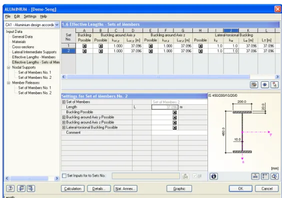
Effective Lengths - Sets of Members

The input table 1.6 controls the effective lengths for sets of members. It is only available if one or more sets of members have been selected in table 1.1 General Data.

Figure 2.15: Table 1.6 Effective Lengths - Set of Members

This table is very similar to the previous table 1.5. With regard to the effective lengths for buckling around the major and minor axes of the cross-sections, it is identical to table 1.5. There are diffenceces, however, with regard to the parameters k_z and k_w for torsional and lateral-torsional buckling. These are used only for straight sets of members if the Member-like Input option is checked in the dialog box Details, Stability tab (cf. Figure 3.2, page 28). Otherwise, the parameters can be defined by specific boundary conditions in tables 1.7 and 1.8 (cf. chapters 2.7 and 2.8) for sets of members not covered by the Member-like Input . If the Member-like Input (cf. Figure 3.2, page 28) is enabled and if the set of members is straight, tables 1.7 and 1.8 are not displayed. The lateral supports can be then defined by intermediate nodes in table 1.4.

Do not use the determination of xs acc. to [1], eq. (6.71) for the lateral-torsional stability design of non-straight sets of members: The bending moments at the start and the end of a set of members can imply misleading values of x_s, ωx and ωxLT and, thus, deviant results.

2.7

Nodal Supports - Sets of Members

The stability design of sets of members is based on the loads and boundary conditions of the selected sets of members. The value of the bifurcation factor αcr has to be determined for the entire set of members in order to obtain critical moment Mcr. The calculation of αcr also depends on the settings in the Details dialog box (cf. chapter 3.1).

To determine αcr, a planar member structure with four degrees of freedom per node is cre-ated. The specific support conditions are defined in table 1.7. This table is only available if you have selected one or more sets of members in table 1.1 General Data.

Figure 2.16: Table 1.7 Nodal Supports - Set of Members

To define the nodal supports, the orientation of the axes within a set of members is im-portant. The program internally checks the location of the relevant nodes and then deter-mines the axis system for the nodal supports that are to be defined in table 1.7 (cf. Figure 2.17 to Figure 2.20).

Figure 2.17: Auxiliary coordinate system for nodal supports – straight set of members

If all the members within the set of members lie on a straight line (Figure 2.17), the local coordinate system of the first member is applied for the entire set of members.

Figure 2.18: Auxiliary coordinate system for nodal supports – set of members in vertical plane

Even if the members within a set do not lie on a straight line, they still must lie in a plane. We can see a vertical plane in Figure 2.18. In this case the axis X’ is horizontal and in the plane direction. The axis Y’ is also horizontal, but perpendicular to the axis X’. The axis Z’ points vertically downwards.

Figure 2.19: Auxiliary coordinate system for nodal supports – set of members in horizontal plane

If the members are located in a horizontal plane (Figure 2.19), the axis X’ is parallel with the axis X of the global coordinate system. The axis Y’ then points in the opposite direction of the global axis Z. The axis Z’ is parallel with the axis Y of the global coordinate system.

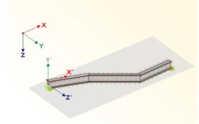
Figure 2.20: Auxiliary coordinate system for nodal supports – set of members in oblique plane

Figure 2.20 shows the most general case. The members within a set of members do not lie on a straight line but are located in an oblique plane. The orientation of the axis X’ is then determined by the intersection between the oblique and the horizontal plane. The axis Y’ is perpendicular to the axis X’ and is also perpendicular to the oblique plane. The axis Z’ is perpendicular to the axes X’ and Y’.

2.8

Member Releases - Sets of Members

This table is only available if one or more sets of members have been selected in table 1.1 General Data. If any member in a given set is not able to transfer internal forces corre-sponding to the degrees of freedom restricted in the table 1.7, then nodal releases can be inserted to a set of members in the table 1.8. There is also possibility to exactly define on which Member Side the release is to act or to place the release at both sides.

Figure 2.21: Table 1.8 Member Releases - Set of Members

If the Member-like Input is enabled (cf. Figure 3.2, page 28) and if the set of members is straight, this table is not displayed. The lateral supports can be defined by intermediate nodes in table 1.4.

2.9

Serviceability Data

The final input table includes different possibilities for the serviceability design. It is only displayed if the serviceability limit state design has been selected in table 1.1 General Data (cf. Figure 2.3).

Figure 2.22: Table 1.9: Serviceability Data

In column A, you can refer the deformation to individual members, list of members or sets of members.

In column B, the relevant members or sets of members can be selected graphically by using the function [Pick]. The reference lengths L in column D are then filled automatically. The Reference Length is set as the length of the member or the entire length of the set resp. list of members. It can be changed Manually by using the corresponding check box in column C and setting the value in column D.

In column E, you specify the governing Direction for the serviceability design. Column F controls whether Precamber wc is to be taken into account as well.

For a correct determination of the serviceability limit states, the Beam Type (beam or canti-lever) is very important. It can be entered in column G.

The settings in the dialog box Details, Serviceability tab controls whether the deformations are referred to the undeformed initial model or to the shifted ends of the members or sets of members (cf. Figure 3.3).

3.

Calculation

3.1

Details

The design is carried out with the internal forces calculated in the RSTAB program. Before the [Calculation], you should check the detailed settings for the design. The corresponding dialog box can be opened from every input or output table by clicking the [Details] button. The Details dialog box consists of four tabs: Ultimate Limit State, Stability, Serviceability and Other.

3.1.1

Ultimate Limit State

Figure 3.1: Dialog box Details, Ultimate Limit State tab

Alternative Values

This dialog section contains a list of parameters that allow for an alternative calculation of values according to EN 1999-1-1. If a box is not checked, the default value will be used. The relevant code clauses are stated for each parameter.

It is possible to choose the default or alternative calculation for each value separately or to use the button [(Un)select All] to set or to remove the check boxes of the whole list.

Options

By default, there is a plastic analysis or elastic analysis in ALUMINIUM – dependent on the class of the cross-section. If required, only the Elastic Design can be activated. Then for all cross-sections classified as 1 or 2 the elastic parameters (as class 3) are used for the design. The Elastic Design of Shear can be used if the shear design is to be based on shear stress in-stead of plastic shear resistance (default).

The Elastic Design of Angles (Based on Stresses) can be applied if the design of angles ac-cording to [1], clauses 6.2.5 to 6.2.10 is to be based on stresses instead of resistance values (default). If this option is checked, the factors ξ0, η0, γ0 and ω0 will be set to 1.00.

Optionally, the Elastic Design of General Cross-sections (Based on Stresses) can be per-formed according to [1], clauses 6.2.5 to 6.2.10 for "general" types such as some sections of the RSTAB library or SHAPE-THIN sections. The design is then based on stresses instead of resistance values (default). Additionally, the Design of General Cross-sections acc. to 6.2.1(5) can be used. This means that the VON MISES yield stresses are calculated in each stress point. The highest ratio according to [1], eq. (6.15) is then used to determine the crit-ical stress point and the final design ratio of each x-location of the member. The parameter C can be set in the National Annex dialog box (see chapter 2.1.3, page 11).

The Design of Plate Girders acc. to 6.7 can be used for cross-sections which fulfill plate girder criteria and are not marked as "general" sections. ALUMINIUM does not support the design of transverse or longitudinal stiffeners, however.

The Shear Design of Solid Cross-sections makes it possible to check shear and bending of massive sections. If this option is not active, bending moments, torsional moment and shear forces are neglected even if they were calculated in RSTAB.

Shear Buckling Design of Webs implies that the design is to be performed according to [1], clauses 6.5.5 and 6.7.4.

The partial factors γM of the materials are controlled in the National Annex dialog box (see chapter 2.1.3, page 11). Please also note that the design of welds (effect of HAZ) is not im-plemented in the current program version.

3.1.2

Stability

Stability Analysis

This section controls whether a stability analysis is to be carried out. If the check is disabled, the input tables 1.4 to 1.8 will not be active.

It can also be specified whether the stability design is to be considered for Bending around the Major and/or Minor Axis. The effects of the 2nd _{Order Theory can be accounted for}

ac-cording to [1], clause 5.2.2(4) by increasing the bending moments by a specific factor. When the check is set, the enlargement factor can be entered. This factor is suited for e.g. a frame whose governing stability failure is lateral buckling. Then, the internal forces can be calculated according to a linear static analysis and then be magnified by suitable factors.

Determination of Elastic Critical Moment for LTB

By default, the elastic critical moment is calculated Automatically by Eigenvalue Method. In this case, an internal model of finite elements is used to determine M_cr with consideration of the following aspects:

• Dimensions of gross cross-section

• Load type and location of load application point

• Real distribution of moments

• Lateral forced deformations (due to support conditions)

• Real boundary conditions

The degrees of freedom of the internal member model are defined by means of the coeffi-cients k_zand k_w (see chapter 2.5).

If the option to determine the elastic critical moment by comparing the Moment Courses is chosen, then the calculation of the coefficient C1 can be controlled in a dialog box which is

accessible via the [Info] button. The coefficients C₂ and C₃ are calculated automatically by the eigenvalue method.

For an unsymmetric section whose shear center has a considerable distance to the centroid in horizonal direction (axis y), a Manual Definition in Table 1.5 of Mcr is recommended. This value can be determined in the FE-LTB module, for example.

The Load Application of Positive Transverse Loads has to be accounted for if those loads have effect on a member. Lateral loads can have stabilizing or destabilizing effects, depend-ing on the application point. This point can be set in the final part of the dialog section. For detailed information on the theoretical background, see [1], Annex I.

Sets of Members - Member-like Input

The stability behavior of sets of members can be analyzed according to three options. It is recommended to apply the ALUMINIUM design only for straight sets of members.

If the default Do not use Member-like Input is set, a general analysis based on the multiplier

αcr is carried out. The support conditions have to be defined in table 1.7 for all sets of members. The factors kz and kw from table 1.6 will not be used.

It is possible to limit the member-like input for Use only for Straight Sets of Members with equal cross-section parameters. The factors kz and kw as defined in table 1.6 are then used to determine the support conditions β, uy, φx, φz and ω. Tables 1.7 and 1.8 will not be dis-played for straight sets. This option can be used e.g. for continuous beams. Please note that the factors kz and kw are identical for every segment or partial member of the set.

The third option applies the member-like input only to Straight Sets of Members without Intermediate Restraints modeled in RSTAB. Thus, only sets of members which have RSTAB supports/restraints at their ends will be considered for the member-like input. This option can be used to design e.g. simple beams or cantilevers. The connection of transverse beams to the intermediate nodes of the set is not accounted for, however. Tables 1.7 and 1.8 will not be displayed for straight sets that have no intermediate supports.

Determination of Distance for Studied Section

The distance xs is defined in [1], figure 6.14. It represents the distance between the studied section and a support or point of contra flexure of deflection curve for elastic buckling of axial force only. It is possible to apply Half of Buckling Length conservatively or to deter-mine xs according to [1], eq. (6.71) for members that have end moments (transverse loads are not admitted). Since the formula provides only one value for x_s, this value will be used in each section of the member.

The application of [1], eq. (6.71) is restricted to linear moment diagrams of the member. Furthermore, the right side has to return a value between –1.0 and 1.0 since the left side of the equation represents a cosine. If one of those two conditions is not fulfilled, the formula will not be applied. Instead, xs is assumed as half of the buckling length for each section. In the current program version, all buckling shapes are considered as unknown. The deter-mination of xs as for known buckling shapes, based on bending moments and rotations, is not implemented.

Limit Load for Special Cases

It is possible to neglect small moments around the major and also the minor axes in order to design unsymmetrical cross-sections of axial compression according to [1], clause 6.3.1. In a similar way, very small axial forces can be neglected so that a bending design without compression according to [1], clause 6.3.2 is possible – by defining the limit ratio N to Npl. Systematic torsion is not accounted for in EN 1999-1-1 adequately. If torsional shear stress-es exist but do not exceed the default limit of 5 %, they will be neglected for the stability design (buckling, lateral buckling).

If any of those limits is exceeded, a message is shown in the results table and the stability design is not carried out. The results of the cross-section design are nevertheless displayed.

Slenderness Determination

Annex I of EN 1999-1-1 provides alternative, simplified procedures how to calculate relative slendernesses for lateral torsional buckling (Annex I.2, clause 2) and torsional and torsional-flexural buckling (Annex I.4, clause 2). Check the appropriate option to enable an alterna-tive calculation.

The alternative calculation of relative slenderness is never used for angles with unequal legs, double angles, cruciforms, cross-sections with fillets or bulbs and general cross-sections.

Torsional and Torsional-Flexural Buckling

Clause 6.3.1.4(1) refers to certain section types that can be neglected for torsional or flex-ural-torsional design: hollow sections, doubly symmetrical I-sections and sections composed of radiating outstands (angles, tees) and classified as class 1 or 2. The check box makes it possible to ignore this type of stability design for the above-mentioned sections.

3.1.3

Serviceability

Figure 3.3: Dialog box Details, Serviceability tab

There are two options in the dialog section Deformation Related to: The selection fields control whether the maximum deformations are to be related to the undeformed, original

model or to an imaginary connecting line between the shifted start and end nodes of the member or set of members within the deformed structure.

The limit deformations can be checked and, if necessary, modified in the National Annex di-alog box (see chapter 2.1.3, page 11).

3.1.4

Other

Figure 3.4: Dialog box Details, Other tab

Cross-section Optimization

Cross-section can be optimized if the Optimize option is chosen in table 1.3 Cross-Sections (see Figure 2.7, page 14). The dialog box Details enables you to set the maximum allowable design ratio as a limit for the optimization process.

Check of Member Slendernesses

It is possible to set user-defined slenderness ratios for members with Tension or Compres-sion / Flexure. These maximum values are compared with the actual member slendernesses in table 3.3. This results table is available after the calculation (see chapter 4.8, page 39) when the corresponding check box is ticked in the Display Results Tables section to the right.

Cross-Section Database

The design of cross-sections which are primarily made of steel (rolled sections) is enabled by default. If this option is unchecked, only cross-sections of the categories Welded, Solid or User-defined will be designed.

Check of Symmetry

This option can be used to make sure whether the cross-section is symmetrical with regard to its principal axis system. Some SHAPE-THIN sections or general RSTAB sections may not be compatible with the design procedure settings of ALUMINIUM where the y-axis is always considered as the major and the z-axis as the minor axis. If, for example, Iy < Iz or the princi-pal axis rotation implies that the z-axis is the major axis, the ALUMINIUM results may be misleading. Therefore, this option can be used to check the symmetry of general sections, independently on the SHAPE-THIN definition. If the symmetry data obtained by both proce-dures are different, an error message will be displayed.

Display Results Tables

In this section, the results tables can be specified which are to be displayed, inclusive of a parts list. The results tables are described individually in chapter 4.

3.2

Start Calculation

In all input tables of ALUMINIUM, you can start the design via the [Calculation] button. At first, ALUMINIUM searches for results of the selected load cases, groups and combina-tions. If they are not found, the calculation of the governing internal forces in RSTAB is started. The calculation parameters of RSTAB are used for this analysis.

If cross-sections are to be optimized (cf. chapter 7.2, page 52), the required sections are calculated and the relevant designs are carried out.

The ALUMINIUM design can be also started from the RSTAB interface. All design cases of the add-on modules are displayed in the To Calculate dialog box, similarly to load cases or load groups. Open this dialog box in RSTAB via the main menu

Calculate →To Calculate.

Figure 3.5: Dialog box To Calculate

If the design cases of ALUMINIUM are missing in the list Not Calculated, it is necessary to tick the check box Show Additional Modules.

The [] button transfers selected design cases to the list on the right. You can then start the calculation by the [Calculate] button.

The calculation of a specific ALUMINIUM design case can also be directly started from the toolbar. Set the relevant design case in the list and then click on the [Results on/off] button.

Figure 3.6: Direct calculation of an ALUMINIUM design case in RSTAB

4.

Results

Table 2.1 Design by Load Case is displayed immediately after the design. In the upper part of this table, a summary of all designs for every load case, load group and combination is displayed. The lower part includes all details of the material properties, design internal forc-es and dforc-esign data of the load case which is selected in the upper part of the table. The results tables 2.1 to 2.5 contain the detailed design summaries according to different selection criteria. Tables 3.1 and 3.2 include the governing internal forces. The parts lists are displayed in the last two tables 4.1 and 4.2.

The results tables are accessible from the navigator in ALUMINIUM. You can also switch among the tables via the buttons as seen to the left or the functional keys [F2] and [F3]. Save the results by the [OK] button and close ALUMINIUM.

In this chapter, the particular tables are described in the given order. The following chapter 5 Evaluation of Results from page 42 onward is devoted to the evaluation and checking of results.

4.1

Design by Load Case

Figure 4.1: Table 2.1 Design by Load Case

Description

The load cases, load groups and combinations that are decisive for every relevant type of design are displayed in this column.

Member No.

The number of the member with the highest design ratio is stated for every designed load case, load group or load combination.

Location x

The location x on the member where the maximum design ratio occurs is displayed in this column. Those locations x on the member are taken into account:

• Start and end nodes

• Internal nodes according to a potential user-defined member division

• Divisions for member results according to settings in RSTAB dialog box Calculation Parameters, Options tab

• Extreme values of internal forces

Design Ratio

For every design type and for every load case, load group or load combination, the design quotients according to the standard are displayed in this column.

The colored bars illustrate the utilizations of every load case.

Design according to Formula

In this column, the equations that were followed in the design are displayed.

DS

The Design Situations which are relevant for the design are stated in the last column: ULS (Ultimate Limit State) or one of the three SLS design situations (CH, FR, QP) as specified in table 1.1 General Data (cf. Figure 2.3, page 10).

4.2

Design by Cross-Section

Figure 4.2: Table 2.2 Design by Cross-section

In this table, the maximum design ratios are displayed for all designed members and for all designed load cases, load groups and combinations. The results are listed according to cross-sections.

4.3

Design by Set of Members

Figure 4.3: Table 2.3 Design by Set of Members

This table is displayed if at least one set of members was selected for design. The maximum design ratios are listed according to sets of members. The number of the member with the highest design ratio within each set of members is shown in column A.

4.4

Design by Member

In this table, the maximum design ratios arranged according to member numbers. The Location x at which the maximum value occurs is stated for every member.

The description of the individual columns can be found in chapter 4.1 on page 34.

4.5

Design by x-Location

Figure 4.5: Table 2.5 Design by x-Location

This results table lists the maximum values of every member at the following locations x ac-cording to the division points of RSTAB:

• Start and end nodes

• Internal nodes according to a potential user-defined member division

• Divisions for member results according to settings in RSTAB dialog box Calculation Parameters, Options tab

4.6

Governing Internal Forces by Member

Figure 4.6: Table 3.1 Governing Internal Forces by Member

Location x

For every member, the location x on the member with the maximum design ratio is shown.

Load Case

In this column, the numbers of the load cases, load groups or combinations whose internal forces have the most unfavorable effects.

Forces / Moments

The decisive axial and shear forces as well as the torsional and bending moments are listed for every member.

Design according to Formula

4.7

Governing

Internal

Forces

by

Set

of

Members

Figure 4.7: Table 3.2 Governing Internal Forces by Set of Member

This results table presents the governing internal forces that lead to the maximum design ratios of every set of members.

4.8

Member Slendernesses

In table 3.3, the effective slenderness ratios of all designed members are compared to the maximum values that were set in the Details dialog box (see chapter 3.1.4, page 31). These ratios are listed with respect to the major and minor principal axes. The table provides in-formation on the maximum effective slenderness ratios only, it does not give any design re-sults.

Members of the types "Tension" or "Cable" are excluded from this table.

4.9

Parts List by Member

Figure 4.9: Table 4.1 Parts List by Member

This table represents a parts list of all cross-sections that are considered in the design case. By default, only designed members are included. If all members of the structure are to be covered, you have to change the relevant setting in the Details dialog box (cf. Figure 3.4, page 31) that can be opened via the [Details] button.

Part No.

The same part number is automatically assigned to identical members.

Cross-section

In this column, the cross-section description is displayed.

Number of Members

The number of identical members is given for each part.

Length

This column displays the unit lengths of every single member.

Total Length

Surface Area

The surface area which is related to the total length of the relevant part is calculated on the basis of the value A_Surf of each cross-section. You can check on this value by clicking on the [Info] button in tables 1.3 or 2.1 to 2.5 (cf. Figure 2.9, page 15).

Volume

The volume of every part is calculated from the surface area and the total length.

Unit Weight

The Unit Weight of the cross-section represents the weight per length of 1 m.

Weight

The value in this column is calculated as the product of values in the columns C and G.

Total Weight

The total weight of each part is displayed in the last column.

Sum

The sums of the values in the individual columns are given in the final row of the list. The cell Total Weight shows the total required amount of steel.

4.10

Parts List by Set of Members

Figure 4.10: Table 4.2 Parts List by Set of Members

The last table in ALUMINIUM is presented when at least one set of members was selected for the design. The advantage of this table is that a parts list is given for the various groups of elements (e.g. for a beam).

The table columns are described in the previous chapter. If there are different cross-sections within the set of members, the mean values of surface area, volume and unit weight are listed here.

5.

Evaluation of Results

The design results can be evaluated in different ways. For this, the buttons in the results ta-bles are very useful. They are located below the upper tata-bles.

Figure 5.1: Buttons for evaluation of results

These buttons have the following functions:

Button Name Function

Design of ultimate limit state

Switch on/off the design results of the ultimate limit state

Design of serviceability limit state

Switch on/off the design results of the servicea-bility limit state

Show color bars in table Switch on/off the color background in the re-sults tables according to the reference scale Show rows with ratio > 1 Show only rows with stress ratios greater than 1

and, accordingly, the failed design Show result diagrams of

current member

Open the diagram Result Diagram on Member  Chapter 5.2, page 45

Jump to graphics to change view

Go to the RSTAB work window in order to change the display settings

Pick member in graphics and go to member in table

Click on a specific member in the RSTAB window whose result values are to be displayed in the ALUMINIUM table

5.1

Results on RSTAB Model

You can use the RSTAB work window to evaluate the design results.

RSTAB Background Graphics and View Mode

The RSTAB graphics in the background can be useful if you want to check the location of a specific member in the model: the member that is selected in the ALUMINIUM results table is also highlighted in the selection color in the RSTAB background graphics. Additionally, an arrow marks the member location x which is stated as decisive in the selected line.

Figure 5.2: Selection of member and current Location x in RSTAB model

If you do not get a favorable view even by moving the ALUMINIUM window, you can apply the so-called View Mode by clicking on the [Change View] button: the ALUMINIUM window is switched off and you can change the view on the RSTAB model. In this mode, the func-tions from the View menu are available, e.g. zoom, move or rotate the view.

Use the [Back] button to return to the ALUMINIUM module.

RSTAB Work Window

The design ratios can be also displayed directly on the structural model. Close ALUMINIUM via the [Graphic] button. The design ratios are then shown graphically in the RSTAB work window.

Similarly to the internal forces in RSTAB, you can activate or deactivate the design results by the [Results on/off] button. The [Show Result Values] button controls the display of the nu-merical values in the graphics.

Regarding the fact that the RSTAB tables are irrelevant to evaluate any ALUMINIUM results, you can deactivate them via the button visible on the left.

A particular design case can be selected from the list of cases in the RSTAB toolbar. The display of results can also be controlled by the Display navigator, using the entry Results → Members. The design ratio is displayed Two Colored by default.

Figure 5.3: Display Navigator: Results → Members → Two Colored

If you select the Colored results display, the color tab of the Panel becomes available that offers various options for the multicolor display. Those are described in chapter 4.4.6 of the RSTAB manual.

Similarly to member internal forces, you can set a scale factor for the graphics of the design ratios in the Factors tab. If you enter the factor 0 in the Member Diagrams input field, the design ratios will be shown with an increased line thickness.

This graphic view can be incorporated to the global printout report (see chapter 6.2, page 48).

You can return to the add-on module any time by clicking on the [ALUMINIUM] button in the panel.

5.2

Result Diagrams

In order to view the detailed distribution of results of a specific member, the graph of re-sults can be used. Select the relevant member (or set of members) in the rere-sults table of ALUMINIUM by placing the cursor in the table line of the member. Then activate the dia-gram by clicking the button as seen to the left. It is located below the upper tables of results (cf. Figure 5.1, page 42).

In the RSTAB window, the result diagrams are available via the main menu

Results → Member Results

or by using the corresponding button in the toolbar.

A new window is opened in which the result diagrams on the selected member or set of members are shown.

Figure 5.5: Result Diagram on Member Dialog

A particular design case can be selected in the list in the toolbar.

The Result Diagram on Member dialog box is described in detail in chapter 9.8.4 of the RSTAB manual on page 206.

5.3

Filtering Results

The structure of the ALUMINIUM tables makes it already possible to select the results ac-cording to certain criteria. Additionally, you can use the filter functions as described in the RSTAB manual to graphically evaluate ALUMINIUM results.

Partial Views

You can use already defined partial views that group specific objects in a suitable way. This function is described in the RSTAB manual, chapter 9.8.6).

Filtering Design Ratios

Secondly, you can set the design ratios as criteria for filtering the results in the RSTAB work window. For this, the so-called control panel is to be displayed. If it is not visible, you can switch it on in the main menu

View →Control panel

or by clicking on the corresponding button in the Results toolbar.

This panel is described in chapter 4.4.6 of the RSTAB manual. The filter settings of the re-sults are defined in the Color Spectrum tab of the panel. If this tab is not available (in case of a two-colored display), it has to be switched on by selecting one of the display options Colored or Cross-sections in the Display navigator.

Figure 5.6: Filtering design ratios with adjusted color spectrum

For a colored view of the results, you can set in the panel that e.g. only design ratios great-er than 0.60 are to be displayed. Furthgreat-ermore, the color spectrum can be adjusted in a way that one color range exactly covers the design ratio 0.10 (see figure above).

By the option Display hidden result diagram (Display navigator, entry Results → Members) you can also display design results that do not satisfy the given condition. Those design di-agrams will then be drawn as dashed lines.

Filtering Members

In the Filter tab of the Panel, you can enter the numbers of the members whose result de-sign ratios are to be shown in the graphics. This function is described in chapter 9.8.6 of the RSTAB manual on page 215.

Figure 5.7: Filtering members to display design ratios of bottom chord

Contrary to the partial view function, the entire structure is displayed. The figure above shows the design ratios in the bottom chord of a footbridge. All other designed members of the structure are displayed in the model, but they are without any design ratios.

6.

Printout

6.1

Printout Report

For all data of ALUMINIUM, a printout report can be created to which you can add graphics and comments. In this printout report, it is also possible to select the input and results ta-bles of ALUMINIUM that are to be printed.

The printout report is described in detail in the manual of RSTAB. In particular, chapter 10.1.3.4 Selecting Data of Add-on Modules on page 227 is important. It deals with the se-lection of input and output data in all add-on modules.

For very large models, it is recommended to use several smaller reports instead of a single extensive one. If you create a specific report only for the ALUMINIUM data, the printout re-port will be processed fairly quickly.

6.2

Print ALUMINIUM Graphics

It is possible to print the design ratios that are displayed on the RSTAB model. All graphics can be incorporated to the printout report or sent directly to the printer. Chapter 10.2 of the RSTAB manual describes in detail how to print graphic displays.

Results on RSTAB Model

Every image of the RSTAB work window can be included in the printout report. The current ALUMINIUM graphics is printed by using the main menu

File → Print…

or by clicking on the corresponding button in the toolbar.

Figure 6.1: Print button in toolbar of main window

Result Diagram

You can also print the result diagrams of members by clicking on the [Print] button in the Result Diagram on Member window.

Figure 6.2: Print button in toolbar of Result Diagram window