Actuarial Statistics With Generalized Linear Mixed Models

Actuarial Statistics With Generalized Linear Mixed

Models

Katrien Antonio

_{Jan Beirlant}

Revision Feburary 2006

Abstract

Over the last decade the use of generalized linear models (GLMs) in actuarial statis-tics received a lot of attention, starting from the actuarial illustrations in the stan-dard text by McCullagh & Nelder (1989). Traditional GLMs however model a sample of independent random variables. Since actuaries very often have repeated measurements or longitudinal data (i.e. repeated measurements over time) at their disposal, this article considers statistical techniques to model such data within the framework of GLMs. Use is made of generalized linear mixed models (GLMMs) which model a transformation of the mean as a linear function of both fixed and random effects. The likelihood and Bayesian approaches to GLMMs are explained. The models are illustrated by considering classical credibility models and more gen-eral regression models for non-life ratemaking in the context of GLMMs. Details on computation and implementation (in SAS andWinBugs) are provided.

Keywords: non-life ratemaking, credibility, Bayesian statistics, longitudinal data, generalized linear mixed models.

∗_{Corresponding author: [email protected] (phone: +32 (0) 16 32 67 69)} †_{Ph. D. student, University Center for Statistics, W. de Croylaan 54, 3001 Heverlee, Belgium.} ‡_{University Center for Statistics, KU Leuven, W. de Croylaan 54, 3001 Heverlee, Belgium.}

1

Introduction

Over the last decade generalized linear models (GLMs) became a common statistical tool to model actuarial data. Starting from the actuarial illustrations in the standard text by McCullagh & Nelder (1989), over applications of GLMs in loss reserving, credibility and mortality forecasting, a whole scala of actuarial problems can be enumerated where these models are useful (see Haberman & Renshaw, 1996, for an overview). The main merits of GLMs are twofold. Firstly, regression is no longer restricted to normal data, but extended to distributions from the exponential family. This enables appropriate modelling of, for instance, frequency counts, skewed or binary data. Secondly, a GLM models the additive effect of explanatory variables on a transformation of the mean, instead of the mean itself. Standard GLMs require a sample of independent random variables. In many actuarial and general statistical problems however the assumption of independence is not fulfilled. Longitudinal, spatial or (more general) clustered data are examples of data structures where this assumption is doubtful. This paper puts focus on repeated measurements and, more specific, longitudinal data, which are repeated measurements on a group of ‘subjects’ over time. The interpretation of ‘subject’ depends on the context; in our illus-trations policyholders and groups of policyholders (risk classes) are considered. Since they share subject-specific characteristics, observations on the same subject over time often are substantively correlated and require an appropriate toolbox for statistical modelling.

Two popular extensions of GLMs for correlated data are the so-called marginal models based on generalized estimating equations (GEEs) on the one hand and the generalized linear mixed models (GLMMs) on the other hand. Marginal models are only mentioned indirectly and do not constitute the main topic of this paper. We focus on the character-istics and applications of GLMMs.

Since the appearance of Laird & Ware (1982) linear mixed models are widely used (e.g. in bio- and environmental statistics) to model longitudinal data. Mixed models extend classical linear regression models by including random or subject-specific effects – next to the (traditional) fixed effects – in the structure for the mean. For distributions from the exponential family, GLMMs extend GLMs by including random effects in the linear predictor. The random effects not only determine the correlation structure between observations on the same subject, they also take account of heterogeneity among subjects, due to unobserved characteristics.

In an actuarial context Frees et al. (1999, 2001) provide an excellent introduction to linear mixed models and their applications in ratemaking. We will revisit some of their illustrations in the framework of generalized linear mixed models. Using likelihood-based hierarchical generalized linear models, Nelder & Verrall (1997) give an interpretation of traditional credibility models in the framework of GLMs. Hierarchical generalized linear models are GLMMs with random effects that are not necessarily normally distributed; an

assumption that is traditionally made. Since the statistical expertise concerning GLMMs is more extensive, this paper puts focus on these models. Apart from traditional credibility models, various other applications are considered as well.

Because both are valuable, estimation and inference in a likelihood-based as well as a Bayesian framework is discussed. In a commercial software package like SAS 1_{, the results} of a likelihood-based analysis are easy to obtain with standard statistical procedures. Our Bayesian implementation relies on Markov Chain Monte Carlo (MCMC) simulations. The results of the likelihood-based analysis can be used for instance to choose starting values for the chains and to check the reasonableness of the results. In an actuarial context, an important advantage of the Bayesian approach is that it yields the posterior predictive distribution of quantities of interest.

Spatial data and generalized additive mixed models (GAMMs) are outside the scope of this paper. Recent work by Denuit & Lang (2004) and Fahrmeir et al.(2003) considers a Bayesian implementation of a generalized additive model (GAM) for insurance data with a spatial structure.

The paper is organized as follows. Section 2 introduces two motivating data sets which will be analyzed later on. In Section 3 we first recall (briefly) the basic concepts of GLMs and linear mixed models. Afterwards GLMMs are introduced and both maximum likeli-hood (i.e. pseudo-likelilikeli-hood or penalized quasi-likelilikeli-hood and (adaptive) Gauss-Hermite quadrature) and Bayesian estimation are discussed. In Section 4 we start with the formu-lation of basic credibility models as particular GLMMs. The crossed classification model of Dannenburg et al. (1996) is illustrated on a data set. Afterwards, illustrations on workers’ compensation insurance data are fully explained. Other interesting applications of GLMMs, for instance in credit risk modelling, are briefly sketched. Finally, Section 5 concludes.

2

Motivating actuarial examples

Two data sets from workers’ compensation insurance are considered. With the intro-duction of these data we want to motivate the need for an extension of GLMs that is appropriate to model correlated –here: longitudinal– data.

2.1

Workers’ Compensation Insurance: Frequencies

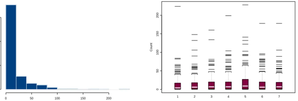
The data are taken from Klugman (1992). Here 133 occupation or risk classes are fol-lowed over a period of 7 years. Frequency counts in workers’ compensation insurance are observed on a yearly basis. Let Count denote the response variable of interest. Possible explanatory variables are Year andPayroll, a measure of exposure denoting scaled payroll

totals adjusted for inflation. Klugman (1992) and later on also Scollnik (1996) and Makov

et al. (1996) have analyzed these data in a Bayesian context (with no explicit formulation

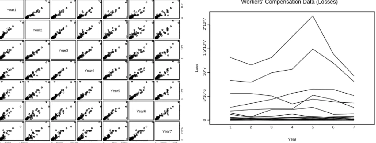
as a GLMM). Exploratory plots for the raw data (not adjusted for exposure) are given in Figure 1 and 2. A histogram of the complete data set and boxplots of the yearly data are shown in Figure 1. The right panel in Figure 2 plots selected response profiles over time and indicates the heterogeneity across the risk classes in the data set. Assuming in-dependence between observations, a Poisson regression model would be a suitable choice since the data are counts. However, the left panel in Figure 2 clearly shows substantive correlation between subsequent observations on the same risk class. Our analysis uses a Poisson GLMM, a choice that will be motivated further in Section 4.

0 50 100 150 200

0

200

400

600

Workers’ Compensation Data (Frequencies)

Count 0 50 100 150 200 1 2 3 4 5 6 7

Workers’ Compensation Data (Frequencies)

Year

Count

Figure 1: Histogram of Count (whole data set) and boxplots of Count for the 7 years in the study, workers’ compensation data (frequencies).

Year1 0 50 100 150 0 50100150200 0 50100150 0 50 150 0 50 100 150 Year2 Year3 0 50 100 0 50 150 Year4 Year5 0 50 150 0 50 150 Year6 050100 200 0 50100 150 050100 200 0 50100150 0 50 150 Year7

Workers’ Compensation Data (Frequencies)

Year Count 0 50 100 150 200 1 2 3 4 5 6 7

Figure 2: Scatterplot matrix of frequency counts (Yeari against Year j for i, j = 1, . . . ,7) (left) and selection of response profiles (right), workers’ compensation data (frequencies).

2.2

Workers’ Compensation Insurance: Losses

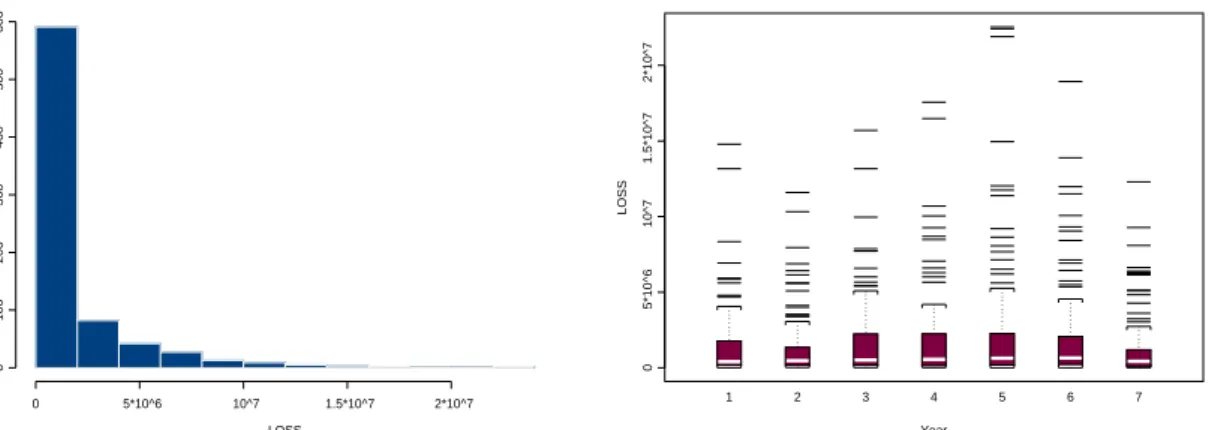
We next consider a data set from the National Council on Compensation Insurance (USA) containing losses due to permanent partial disability. As with the previous illustration, Klugman (1992) already analyzed these data to illustrate the possibilities of Bayesian statistics in non-life ratemaking. 121 occupation or risk classes are observed over a period of 7 years. The variable Loss gives the amount of money paid out (on a yearly basis). Possible explanatory variables are Year and Payroll. The data also appeared in Frees

et al. (2001) where the pure premium, PP=Loss/Payroll, was used as response variable.

Figure 3 contains exploratory plots for the variable Loss. The right-skewness of boxplot and histogram is apparent. Figure 4 reveals substantive correlation between subsequent observations on the same risk class. In Section 4 a gamma GLMM is used to model these longitudinal data in the GLM framework.

0 5*10^6 10^7 1.5*10^7 2*10^7 0 100 200 300 400 500 600

Workers’ Compensation Data (Losses)

LOSS 0 5*10^6 10^7 1.5*10^7 2*10^7 1 2 3 4 5 6 7

Workers’ Compensation Data (Losses)

Year

LOSS

Figure 3: Histogram of Loss (whole database) and boxplots of Loss for the 7 years in the study, workers’ compensation data (losses).

3

GLMMs for actuarial data

3.1

Basic concepts of GLMs and linear mixed models

For the reader’s convenience, we provide a short summary of the main characteristics of GLMs on the one hand and mixed models on the other hand, before introducing their extension to GLMMs. For a broad introduction to generalized linear models (GLMs) we refer to McCullagh & Nelder (1989). Numerous illustrations of the use of GLMs in typi-cal problems from actuarial statistics are available; see e.g. Haberman & Renshaw (1996). Full details on linear mixed models can be found in Verbeke & Molenberghs (2000) or Demidenko (2004). Frees et al. (1999) give a good introduction to the possibilities of

Year1 0 4*10^6 10^7 05*10^6 1.5*10^7 0 10^7 0 10^7 0 6*10^6 Year2 Year3 0 10^7 0 10^7 Year4 Year5 0 10^7 0 10^7 Year6 0 5*10^6 1.5*10^7 0 5*10^6 1.5*10^7 0 10^7 2*10^7 0 4*10^6 10^7 0 6*10^6 Year7

Workers’ Compensation Data (Losses)

Year Loss 0 5*10^6 10^7 1.5*10^7 2*10^7 1 2 3 4 5 6 7

Figure 4: Scatterplot matrix of losses, Year i against Year j for i, j = 1, . . . ,7 (left) and selection of response profiles (right), workers’ compensation data (losses).

linear mixed models in actuarial statistics.

Generalized Linear Models (GLMs)

A first important feature of GLMs is that they extend the framework of general (nor-mal) linear models to the class of distributions from the exponential family. A whole variety of possible outcome measures (like counts, binary and skewed data) can be mod-elled within this framework. This paper uses the canonical form specification of densities from the exponential family, namely

f(y) = exp µ yθ−ψ(θ) φ +c(y, φ) ¶ (1) where ψ(.) and c(.) are known functions, θ is the natural and φ the scale parameter. LetY1, . . . , Yn be independent random variables with a distribution from the exponential

family. The following well-known relations can easily be proven for such distributions

µi = E[Yi] =ψ

0

(θi) and Var[Yi] = φψ

00

(θi) = φV(µi) (2)

where derivatives are with respect to θ and V(.) is called the variance function. This function captures the relationship, if any exists, between the mean and variance of Y.

A second important feature of GLMs is that they provide a way around the transfor-mation of data. Instead of a transformed data vector, a transfortransfor-mation of the mean is modelled as a linear function of explanatory variables. In this way

g(µi) =ηi = (Xβ)i (3)

where β = (β1, . . . , βp)

0

contains the model parameters and X (n × p) is the design matrix. g is the link function and ηi is the ith element of the so-called linear predictor.

The unknown but fixed regression parameters inβare estimated by solving the maximum likelihood equations with an iterative numerical technique (such as Newton-Raphson). Likelihood ratio and Wald tests are used for inference purposes. If the scale parameter φ

is unknown, it can be estimated either by maximum likelihood or by dividing the deviance or Pearson’s chi-square statistic by its degrees of freedom.

GLMs are well suited to model various outcomes from cross-sectional experiments. In a cross-sectional data set a response is measured only once per subject, in contrast to longitudinal data. Longitudinal (but also clustered or spatial) data require appropriate statistical tools as it should be possible to model correlation between observations on the same subject (same cluster or adjacent regions). Since Laird & Ware (1982) mixed models became a popular and widely used tool to model repeated measurements in the framework of normal regression models. Before discussing the extension of GLMs to GLMMs, we recall the main principles of linear mixed models.

Linear Mixed Models (LMMs)

Linear mixed models extend classical linear regression models by incorporating random effects in the structure for the mean. Assume the data set at hand consists ofN subjects. Let ni denote the number of observations for the ith subject. Yi is the ni×1 vector of

observations for the ith _{subject (1≤i≤N). The general linear mixed model is given by}

Yi =Xiβ+Zibi+²i. (4)

β (p×1) contains the parameters for the p fixed effects in the model; these are fixed, but unknown, regression parameters, common to all subjects. bi (q×1) is the vector

with the random effects for the ith _{subject in the data set. The use of random effects}

reflects the belief that there is heterogeneity among subjects for a subset of the regression coefficients inβ. Xi (ni×p) andZi (ni×q) are the design matrices for thepfixed andq

random effects. ²i (ni×1) contains the residual components for subject i. Independence

between subjects is assumed. bi and ²i are also assumed to be independent and we follow

the traditional assumption that they are normally distributed with mean vector 0 and covariance matrices, say D (q×q) andΣi (ni×ni), respectively. Different structures for

these covariance matrices are possible; an overview of some frequently used ones can be found in Verbeke & Molenberghs (2000). It is easy to see that Yi then has a marginal

normal distribution with mean Xiβ and covariance matrix Vi = Var(Yi), given by

Vi =ZiDZ

0

i+Σi. (5)

In this interpretation it becomes clear that the fixed effects enter only the mean E[Yij],

whereas the inclusion of subject-specific effects specifies the structure of the covariance between observations on the same unit.

Denote the unknown parameters in the covariance matrixVi withα. Conditional on

α, a closed form expression for the maximum likelihood estimator of β exists, namely

ˆ β= ( N X i=1 X0_iV−_i 1Xi)−1 N X i=1 X0_iV−_i 1Yi. (6)

To predict the random effects the mean of the posterior distribution of the random effects given the data, bi|Yi, is used. Conditional on α, we have

ˆ

bi =DZ

0

iV−i 1(Yi−Xiβ)ˆ , (7)

which can be proven to be the Best Linear Unbiased Predictor (BLUP) ofbi (where ‘best’

is again in the sense of minimal mean squared error). For estimation ofαmaximum likeli-hood (ML) or restricted maximum likelilikeli-hood (REML) is used. The expression maximized by the ML (L1), respectively REML (L2), estimates is given by

L1(α;y1, . . . ,yN) = c1− 1 2 N X i=1 log|Vi| − 1 2 N X i=1 r0_iV−1 i ri (8) L2(α;y1, . . . ,yN) = c2− 1 2 N X i=1 log|Vi| − 1 2 N X i=1 log|X0_iV−1 i Xi| − 1 2 N X i=1 r0_iV−1 i ri,(9) where ri = yi − Xi ³P_N i=1X 0 iViXi ´_−1³P N i=1X 0 iV−i 1yi ´

and c1, c2 are appropriate constants. Equations (8) and (9) are maximized using iterative numerical techniques such as Fisher scoring or Newton-Raphson (check Demidenko, 2004, for full details). In (6) and (7) the unknownαis then replaced with ˆαM L or ˆαREM L, leading to the empirical BLUE

forβand the empirical BLUP forbi. For inference regarding the fixed and random effects

and the variance components, appropriate likelihood ratio and Wald tests are explained in Verbeke & Molenberghs (2000).

3.2

GLMMs: model specification

GLMMs extend GLMs by allowing for random, or subject-specific, effects in the linear predictor (3). These models are useful when the interest of the analyst lies in the individual response profiles rather than the marginal mean E[Yij]. The inclusion of random effects

in the linear predictor reflects the idea that there is natural heterogeneity across subjects in (some of) their regression coefficients. This is the case for the actuarial illustrations discussed in Section 4. Diggleet al.(2002), McCulloch & Searle (2001), Demidenko (2004) and Molenberghs & Verbeke (2005) are useful references for full details on GLMMs.

Say we have a data set at hand consisting ofN subjects. For each subjecti(1≤i≤N)

ni observations are available. Given the vectorbi with the random effects for subject (or

density from the exponential family f(yij|bi,β, φ) = exp µ yijθij−ψ(θij) φ +c(yij, φ) ¶ , j = 1, . . . , ni. (10)

Similar to (2), the following (conditional) relations hold

µij = E[Yij|bi] =ψ 0 (θij) and Var[Yij|bi] = φψ 00 (θij) = φV(µij) (11) where g(µij) = x 0 ijβ +z 0

ijbi. As before, g(.) is called the link and V(.) the variance

function. β (p×1) denotes the fixed effects parameter vector andbi (q×1) the random

effects vector. xij (p×1) and zij (q×1) contain subject i’s covariate information for

the fixed and random effects, respectively. The specification of the GLMM is completed by assuming that the random effects, bi (i = 1, . . . , N), are mutually independent and

identically distributed with density function f(bi|α). Hereby α denotes the unknown

parameters in the density. Traditionally, one works under the assumption of (multivariate) normally distributed random effects with zero mean and covariance matrix determined by α. Correlation between observations on the same subject arises because they share the same random effects bi.

The likelihood function for the unknown parameters β, α and φ then becomes (with y= (y0₁, . . . ,y0_n)0) L(β,α, φ;y) = N Y i=1 f(y_i|α,β, φ) = N Y i=1 Z Yni j=1 f(yij|bi,β, φ)f(bi|α)dbi, (12)

where the integral is with respect to the q dimensional vector bi. When both the data

and the random effects are normally distributed (as in the linear mixed model), the integral can be worked out analytically and closed-form expressions exist for the maximum likelihood estimator of β and the BLUP for bi (see (6) and (7)). For general GLMMs,

however, approximations to the likelihood or numerical integration techniques are required to maximize (12) with respect to the unknown parameters. These will be sketched briefly in a following subsection and discussed in more detail in Appendix A.

For illustration, we consider a Poisson GLMM with normally distributed random in-tercept. This GLMM allows explicit calculation of the marginal mean and covariance matrix. In this way one can clearly see how the inclusion of the random effect models over-dispersion and within-subject covariance in this example.

Example: a Poisson GLMM Let Yij denote the jth observation for subject i.

exp (x0_ijβ+bi) and that bi ∼N(0, σb2). Straightforward calculations lead to

Var(Yij) = Var(E(Yij|bi)) + E(Var(Yij|bi))

= E(Yij)(exp (x

0

ijβ)[exp (3σ2b/2)−exp (σb2/2)] + 1), (13)

and

Cov(Yij1, Yij2) = Cov(E(Yij1|bi),E(Yij2|bi)) + E(Cov(Yij1, Yij2|bi))

= exp (x0_ij1β) exp (x0_ij2β)(exp (2σ2

b)−exp (σ2b)). (14)

Hereby we used the expressions for the mean and variance of a lognormal distribution. We see that the expression in round parentheses in (13) is always greater than 1. Thus, although Yij|bi follows a regular Poisson distribution, the marginal distribution of Yij is

over-dispersed. According to (14), due to the random intercept, observations on the same subject are no longer independent.

GLMMs are appropriate for statistical problems where the modelling and prediction of individual response profiles is of interest. However, when interest lies only in the pop-ulation average (and the effect of explanatory variables on it), so-called marginal models (see Diggle et al., 2002 and Molenberghs & Verbeke, 2005) extend GLMs for indepen-dent data to models for clustered data. For instance, when using Generalized Estimating Equations, the effect of explanatory variables on the marginal expectation E[Yij] (instead

of the conditional expectation E[Yij|bi] as in (11)) is specified and –separately– a ‘working’

assumption for the association structure is assumed. The regression parameters inβthen give the effect of the corresponding explanatory variables on the population average. In a GLMM however these parameters represent the effect of the explanatory variables on the responsesfor a specific subject and (in general) they do not have a marginal interpretation. For, E[Yij] = E[E[Yij|bi]] = E[g−1(x 0 ijβ+z 0 ijbi)]6=g−1(x 0 ijβ).

3.3

Parameter estimation, inference and prediction

In general, the integral in (12) can not be evaluated analytically. The normal-normal case (normal distribution for the response as well as random effects) is an exception. More general situations require either model approximations or numerical integration tech-niques to obtain likelihood-based estimates for the unknown parameters. This paragraph gives a very brief introduction to restricted pseudo-likelihood ((RE)PL) (Wolfinger & O’Connell, 1993) and (adaptive) Gauss-Hermite quadrature (Liu & Pierce, 1994) to per-form the maximum likelihood estimation. Both techniques are available in the commercial software package SAS and their use will be illustrated later on. The pseudo-likelihood technique corresponds with the penalized quasi-likelihood (PQL) method of Breslow & Clayton (1993). Since maximum likelihood techniques are hindered by the integration over the q-dimensional vector of random effects, a Bayesian implementation of GLMMs

is considered as well. Hereby random numbers are drawn from the relevant posterior and predictive distributions using Markov Chain Monte Carlo (MCMC) techniques. Win-Bugs allows easy implementation of these models. To make this article self-contained a first introduction to technical details is bundled in Appendix A. Illustrative code for both SAS and WinBugs is available on the web 2_.

3.3.1 Maximum likelihood approach

(Restricted) Pseudo-likelihood ((RE)PL)

Using a Taylor series the pseudo-likelihood technique approximates the original GLMM by a linear mixed model for pseudo-data. In this linearized model the maximum likelihood estimators for the fixed effects and BLUPs for the random effects are obtained using the well-known theory for linear mixed models (as outlined in Section 3.1). The advantage of this approach is that a large number of random effects but also crossed and nested random effects can be handled. A disadvantage is that no true log-likelihood is used. Therefore likelihood-based statistics should be interpreted with great caution. Moreover the estimation process is doubly iterative; a linear mixed model is fit, which is an iterative process, and this procedure is repeated until the difference between subsequent estimates is sufficiently small. In SAS the macro %Glimmix 3 _{and procedure Proc Glimmix} 4 enable pseudo-likelihood estimation. Justifications of the approach are given by Wolfinger & O’Connell (1993) and Breslow & Clayton (1993) (via Laplace approximation) where the approach is called Penalized Quasi-Likelihood (PQL).

(Adaptive) Gauss-Hermite quadrature

Non-adaptive Gauss-Hermite quadrature is an example of a numerical integration tech-nique that approximates any integral of the form

Z _+∞

−∞

h(z) exp (−z2_{)dz (15)}

by a weighted sum, namely

Z _+∞ −∞ h(z) exp (−z2_{)dz ≈} Q X q=1 wqh(zq). (16)

Here Q denotes the order of the approximation, the zq are the zeros of the Qth order

Hermite polynomial and the wq are corresponding weights. The nodes (or quadrature 2_{see http://www.econ.kuleuven.be/katrien.antonio}

3_{available athttp://ftp.sas.com/techsup/download/stat/} 4_{experimental version available as an add-on to SAS 9.1}

points) zq and the weights wq are tabulated in Abramowitz & Stegun (1972, page 924).

By using an adaptive Gauss-Hermite quadrature rule the nodes are rescaled and shifted such that the integrand is sampled in a suitable range. Details on (adaptive) Gauss-Hermite quadrature are given in Liu & Pierce (1994) and are summarized in Appendix A.2. This numerical integration technique still enables for instance a likelihood ratio test. Moreover the estimation process is just singly iterative. On the other hand, at present, the procedure can only deal with a small number of random effects which limits its general applicability. (Adaptive) Gauss-Hermite quadrature is available in SAS via Proc Nlmixed.

3.3.2 Bayesian approach

The maximum likelihood techniques presented in the previous section are complicated by the integration over the q-dimensional vector of random effects. Therefore we also consider a Bayesian implementation of GLMMs, which enables the specification of com-plicated structures for the linear predictor (combining, for instance, a lot of random effects, or crossed and nested effects). Another advantage of the Bayesian approach is that various (other than the normal) distributions can be used for the random effects, whereas in cur-rent statistical software (like SAS) only normally distributed random effects are available, though use of the EM algorithm enables other specifications like a Student t-distribution or a mixture of normal distributions.

The Bayesian approach treats all unknown parameters in the GLMM as random vari-ables. Prior distributions are assigned to the regression parameters inβand the covariance matrix D of the normal distribution for the random effects. Since the posterior distribu-tions involved in GLMMs are typically numerically and analytically intractable, posterior and predictive inference is based on drawing random samples from the relevant posterior and predictive distributions with Markov Chain Monte Carlo (MCMC) techniques. An early reference to Gibbs sampling in GLMMs is Zeger & Karim (1991).

For the examples in Section 4, the following distributional and prior specifications are used (canonical link for ease of notation):

[Y|b] = exp{y0(Xβ+Zb)−10ψ(Xβ+Zb) +10c(y)}, (17) where Y = (Y0₁, . . . ,Y0_N)0, b = (b0₁, . . . ,b0_N)0 and X, Z are the corresponding design matrices. Further,

[b]∼N(0,blockdiag(G)), [β]∼N(0,F), [G]∼Inv-Wishartν(B), (18)

where F is a diagonal matrix with large entries and B has the same dimensions as G. These specifications result in the following full conditionals

[β|.] ∝ exp{y0Xβ−10ψ(Xβ+Zb)− 1

2β

0

[b|.] ∝ exp{y0Zb−10ψ(Xβ+Zb)− 1 2b 0 G−1_{b}, (20)} [G|.] ∝ Inv-Wishartν+N(B+ N X i=1 bib 0 i). (21)

For a single variance component, an inverse gamma prior is used, which results in an inverse gamma full conditional. In the sequel of this article, the WinBugs software is used for Gibbs sampling. Zhaoet al. (2005) give more technical details on Gibbs sampling in GLMMs.

3.3.3 Inference and Prediction

In actuarial regression problems (see Section 2) accurate prediction for individual risk classes is of major concern. Since Bayesian statistics allows simulation from the full predictive distribution of any quantity of interest, this approach is the most appealing from this point of view. In Section 4.2.2 also predictions obtained with Proc Glimmix and Proc Nlmixed are displayed. With Proc Glimmix we report g−1_(ˆη

i,ni+1) for

the predicted value and

q

Var(g−1_(ˆη

i,ni+1−z

0

i,ni+1bi)) for the prediction error. Hereby

ˆ

ηi,ni+1 =x 0

i,ni+1βˆ+z

0

i,ni+1ˆbi and the delta method is applied to Var

" ˆ β ˆ bi−bi # , obtained from the final Proc Mixed call. With Proc Nlmixed, predicted values are computed from the parameter estimates for the fixed effects and empirical Bayes predictors for the random effects. Standard errors of prediction for some function of the fixed and random effects (say, g−1_(x0

i,ni+1βˆ +z

0

i,ni+1ˆbi)) are again obtained with the delta method

and an approximate prediction variance matrix for

" ˆ β ˆ bi #

. For Var(ˆβ) the inverse of an approximation of the corresponding Fisher information matrix is used. For the variance of ˆ

bi,Proc Nlmixeduses an approximation to Booth & Hobert’s (1998) conditional mean

squared error of prediction. The predictions and prediction errors reported in Section 4.2.2, obtained with PQL and G-H respectively, are very close.

4

Applications

4.1

A GLMM interpretation of traditional credibility models

The credibility ratemaking problem is concerned with the determination of a risk premium for a group of contracts which combines the claims experience related to that specific group and the experience regarding related risk classes. This approach is justified since the risks in a certain class have characteristics in common with risks in other classes, but they also have their own risk class specific features. For a general introduction to

classical credibility theory, we refer to Dannenburg et al. (1996). Using linear mixed models Frees et al. (1999) already gave a longitudinal data analysis interpretation of the well-known credibility models of B¨uhlmann (1967,1969), B¨uhlmann-Straub (1970), Hachemeister (1975) and Jewell (1975). They explained how to specify the fixed (β) and random effects (bi) for every subject or risk classi (i= 1, . . . , N) and used βb and bbi (as

in (6) and (7)) to derive the Best Linear Unbiased Predictor for the conditional mean of a future observation (E[Yi,ni+1|bi]). For the above mentioned credibility models, this BLUP

corresponds with the classical credibility formulas (as in Dannenburg et al., 1996). However, the normal-normal model (normality for both responses and random effects) will not always be plausible for the data at hand (which can be, for instance, counts, binary or skewed data). Therefore it is useful to revisit the credibility models in the context of GLMs and to consider their specification as a GLMM. In this way estimators and predictors will be used that take the distributional features of the data into account. For GLMMs (in general) no closed-form expressions forβˆ andˆbi exist and one has to rely

on the techniques presented in Section 3.3 to derive a predictor for E[Yi,ni+1|bi].

The interpretation of actuarial credibility models as (generalized) linear mixed mod-els has several advantages over the traditional approach. For instance, the inferential tools from the theory of mixed models can be used to check the models. Moreover, the likelihood-based estimation of fixed effects and unknown parameters in the covariance structure is well-developed in the framework of (G)LMMs, which provides an alternative for the traditional moment-based estimators used in actuarial literature (see Dannenburg

et al., 1996).

Whereas this paper puts focus on statistical aspects of GLMMs and their use in the modelling of real data sets, Purcaru & Denuit (2003) studied the kind of dependence that arises from the inclusion of random effects in credibility models for frequency counts, based on GLMs.

4.1.1 Mixed model specification of well-known credibility models

Interpreting traditional credibility models in the context of GLMMs implies that the additive regression structure in terms of fixed and subject-specific (or risk class specific) effects is specified on the scale of the linear predictor, namely

g(µij) = ηij =x

0

ijβ+z

0

ijbi. (22)

Hereby i (i = 1, . . . , N) denotes the subject, for instance a policy(holder) or risk class, and j refers to its jth _{measurement, unless it is stated otherwise. The link function g(.)}

and variance function V(.) are determined by the chosen GLM. Next to the above men-tioned models of B¨uhlmann (1967, 1969), B¨uhlmann-Straub (1970), Hachemeister (1975) and Jewell (1975), we also consider the crossed classification model of Dannenburg et al.

1. B¨uhlmann’s model

Expression (22) becomes g(µij) = ηij =β +bi (for i = 1, . . . , N). Thus, on the scale of

the linear predictor, a single fixed effectβ denotes the overall mean and the random effect

bi denotes the deviation from this mean, specific for contract or policyholder i.

2. B¨uhlmann-Straub’s model

B¨uhlmann’s model is extended by introducing (known) positive weights. In the GLMM specification weights are introduced by replacing φwithφ/wij inf(yij|β,bi, φ) (see (10)).

The structure of the linear predictor from B¨uhlmann’s model remains unchanged. The importance of including weights is already discussed in Kaas et al.(1997).

3. Hachemeister’s model

Hachemeister’s model is a credibility regression model and generalizes B¨uhlmann’s model by introducing collateral data. The structure for the linear predictor is obtained by tak-ing x0_ij = z0_ij in (22). For instance, xit = zit = (1 t)

0

leads to the linear trend model considered in Frees et al. (1999).

4. Jewell’s hierarchical model

This hierarchical model classifies the original set of N policies or subjects according to a certain number of risk factors. Consider for instance the mixed model formulation for a

two-stage hierarchy. We have that g(µijt) =ηijt=β+bi+bij. Hereby i denotes the risk

factor at the highest level andj denotes the categories of the second risk factor. tindexes the repeated measurements for this (i, j) combination. bi is a random effect for the first

risk factor. The random effect bij characterizes categoryj of the second risk factor within

the ith _{category of the highest risk factor. More than two nestings can be dealt with in}

the same manner.

5. Dannenburg’s crossed classification model

Crossed classification models are an extension of the hierarchical models studied by Jewell (1975) and also allow risk factors to occur next to each other, instead of fully nested. For instance, in the two-stage hierarchy described above, there is no risk factor which char-acterizes the second stage, without interacting with the first stage. Dannenburg’s model (Dannenburget al., 1996) allows a combination of crossed and nested random effects and specifies the linear predictor for the two-way model as ηijt=β+b(1)i +b

(2)

j +b

(12)

ij , where

4.2

Data Examples

Three examples are discussed where GLMMs are used to model real data. In a first example Dannenburg’s crossed classification model is considered. Afterwards, the data introduced in Section 2 are analyzed.

4.2.1 Dannenburg’s Crossed Classification Model

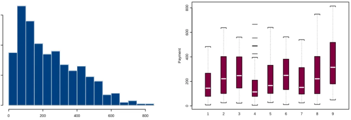
We consider the data from Dannenburg et al.(1996, page 108). The crossed classification model is illustrated on a two-way data set made available by a credit insurer. The data are payments of this credit insurer to several banks in order to cover losses caused by clients who were not able to pay off their private loans. The observations have been categorized according to marital status of the debtor and the time he worked with his current employer. On every cell (i.e. a status-experience combination) repeated measurements are available. Exploratory plots are given in Figure 5. Scollnik (2000) considered the same data set to illustrate a Bayesian implementation of the crossed classification model (under normality for the response). We believe that it is illustrative to analyze these data again, since we explicitly consider this credibility model as a GLMM and illustrate how to estimate parameters and risk premia using likelihood-based as well as Bayesian techniques.

Leti denote the marital status of the debtor (1=single, 2=divorced and 3=other) and

j the time he worked with his current employer (1=less than 2 years, 2=between 2 and 10 years and 3=more than 10 years). Dannenburg et al. (1996) modelled these data as

Yijt =β+b(1)i +b(2)j +b(12)ij +²ijt, where t refers to the tth observation in cell (i, j). The

original crossed classification model assumes all the random components to be mutually independent with zero mean and δ1 = Var(b(1)i ), δ2 = Var(b(2)j ), δ12 = Var(b(12)ij ) and

σ2 _{= Var(²}

ijt). Dannenburg et al. (1996) had to rely on typical (complicated) credibility

calculations to obtain estimates for the risk premia in terms of credibility factors and weighted averages of the observations in the different cells or levels. These are functions of the unknown variance components and overall mean (β) for which moment-based es-timators are proposed. The theory of mixed models is useful here since it provides a unified framework to perform the estimation of the regression parameter β and variance components δ1, δ2, δ12 and σ2, together with the prediction of the random effects.

As illustrated clearly by Figure 5, the data are right-skewed. In contrast to Scollnik (2000) we analyzed the data with a gamma GLMM with logarithmic link function and normality for the random effects. We initially specified the linear predictor as ηijt =

β+b(1)_i +b(2)_j +b(12)_ij , but the variance component corresponding with the interaction term was put equal to zero by the procedure. This is in line with the findings in Dannenburg et al. (1996, page 106). Thus, the model is reduced to a two-way model without interaction and a linear predictor of the form ηijt = β +b(1)i +b(2)j . We fit this model using the

via the SAS macro %Glimmix and the SAS procedure Proc Glimmix. The results are given in Table 1 and 2. Note that a test for the need of the random effects involves a boundary problem (H0 : δ1 = 0 versus H1 : δ1 > 0, for instance) and would, with our model specification, rely on Monte Carlo simulations. For prediction purposes, a Bayesian implementation of the model is extremely useful. Figure 6 shows histograms for simulations from the predictive distribution of Yij,nij+1 for every (i, j) combination.

0 200 400 600 800

0

20

40

60

Dannenburg’s Cross-Classification Model

Payment 0 200 400 600 800 1 2 3 4 5 6 7 8 9

Dannenburg’s Cross-Classification Model

Combination of Experience and Status

Payment

Figure 5: Histogram of ‘Payment’ (whole database) and boxplots of ‘Payment’ for each

(i, j) combination (1=(1,1), 2=(1,2), 3=(1,3), 4=(2,1), 5=(2,2), 6=(2,3), 7=(3,1),

8=(3,2), 9=(3,3)). i gives the marital status (1=single, 2=divorced, 3=other) and j

the time worked with current employer (1 : <2 yrs,2 : ≥2 and ≤10 yrs,3 : >10yrs).

Effect Parameter Estimate (s.e.)

Fixed-effects parameter

Intercept β 5.475 (0.146)

Variance parameters

Class i δ1 0.014 (0.018)

Class j δ2 0.046 (0.045)

Table 1: Gamma-normal mixed model with logarithmic link function: estimates for fixed effect and variance components (under REML), credit insurer data. Results obtained with

Proc Glimmix in SAS.

4.2.2 Workers’ Compensation Insurance: Frequencies

Background for this data set is given in Section 2.1 and exploratory plots are shown in Figure 1 and 2. We analyze the data using mixed models and build up suitable regression models in this context. Since the data are frequency counts and interest lies in predictions

j = 1 j = 2 j = 3

i= 1 183 239 275

i= 2 176 230 265

i= 3 215 281 323

Table 2: Gamma-normal mixed model: estimated risk premia based on the estimate for

the fixed effect and predictions for the random effects using SAS Proc Glimmix, credit

insurer data. 0 200 400 600 800 1200 0 500 1500 Premium 1 0 500 1000 1500 0 1000 2500 Premium 2 0 500 1000 1500 0 1000 2000 Premium 3 0 200 400 600 800 1000 0 500 1500 Premium 4 0 200 400 600 8001000 0 500 1500 Premium 5 0 500 1000 1500 2000 0 1000 2500 Premium 6 0 200 400600 800 1200 0 500 1500 Premium 7 0 500 1000 1500 0 1000 2000 Premium 8 0 500 1000 1500 2000 0 500 1500 Premium 9

Figure 6: Predictive distributions for different risk classes, credit insurer data. Burn-in of 50,000 simulations, followed by another 50,000 simulations.

regarding individual risk classes, our analysis uses a Poisson GLMM. Heterogeneity across risk classes and correlation between observations on the same class further motivate the inclusion of random effects in the linear predictor of the Poisson GLM.

The following models are considered

Yij|bi ∼ Poisson(µij)

where log (µij) = log (Payrollij) +β0+β1Yearij +bi,0 (23) versus log (µij) = log (Payrollij) +β0+β1Yearij +bi,0+bi,1Yearij. (24)

Hereby Yij represents the jth measurement on the ith subject of the response Count. β0 and β1 are fixed effects and bi,0, versus bi,1, is a risk class specific intercept, versus slope. It is assumed that bi = (bi,0, bi,1)

0

are independent. The results of both a maximum likelihood and a Bayesian analysis are given in Table 3. The models were fitted to the data set without the observed Counti7, to enable out-of-sample prediction later on. In Table 3, δ0 = Var(bi,0),δ1 = Var(bi,1) and

δ0,1 = δ1,0 = Cov(bi,0, bi,1). Proc Glimmix did not converge with model specification (24), together with a general structure for the covariance matrixD of the random effects. For the adaptive Gauss-Hermite quadrature 20 quadrature points were used in SASProc Nlmixed, though for example, an analysis with 5, 10 and 30 quadrature points gave practically indistinguishable results. For the prior distributions in the Bayesian analysis we used the specifications from Section 3.3.2. Four parallel chains were run and for each chain a burn-in of 20,000 simulations was followed by another 50,000 simulations. As reported by many authors (see for instance Zhao et al., 2005) centering of covariates and hierarchical centering greatly improves mixing of the chains and speed of simulation.

PQL adaptive G-H Bayesian

Est. SE Est. SE Mean 90% Cred. Int.

Model (23) β0 -3.529 0.083 -3.557 0.084 -3.565 (-3.704, -3.428) β1 0.01 0.005 0.01 0.005 0.01 (0.001, 0.018) δ0 0.790 0.110 0.807 0.114 0.825 (0.648, 1.034) Model (24) β0 -3.532 0.083 -3.565 0.084 -3.585 (-3.726, -3.445) β1 0.009 0.011 0.009 0.011 0.008 (-0.02, 0.04) δ0 0.790 0.111 0.810 0.115 0.834 (0.658, 1.047) δ1 0.006 0.002 0.006 0.002 0.024 (0.018, 0.032) δ0,1 / / 0.001 0.01 0.006 (-0.021, 0.034)

Table 3: Workers’ compensation data (frequencies): results of maximum likelihood and Bayesian analysis. REML is used in PQL.

To check whether model (24) can be reduced to (23), a likelihood ratio test for the need of random slopes was used and resulted in an observed value of 74=4394-4320 (with adaptive G-H quadrature, 20 quadrature points). Figure 7 illustrates that the fitted values obtained with the preferred model (24) are close to the real observed values. To illustrate prediction with this model, Table 4 compares the predictions for some selected risk classes with the observed values. These risk classes are the same as in Klugman (1992) and Scollnik (1996). The predicted values are calculated as exp (µci7) (i= 11,20,70,89,112). The reported prediction errors are obtained as described in Section 3.3.3. As mentioned in the same section, when focus lies on prediction, the Bayesian approach is the most useful, since it provides the full predictive distribution of Yi7. For the selected risk classes,

Workers’ Compensation Insurance: Frequencies Observed Fitted 0 50 100 150 200 0 50 100 150 200

Figure 7: Workers’ compensation data (frequencies): scatterplot of observed counts versus

fitted values for Model (24), via SAS Proc Nlmixed.

these predictive distributions are illustrated in Figure 8.

Actual Values Expected number of claims

PQL adaptive G-H Bayesian

Class Payroll_i7 Counti7 Mean s.e. Mean s.e. Mean 90% Cred. Int.

11 230 8 11.294 2.726 11.296 2.728 12.18 (5,21)

20 1,315 22 33.386 4.109 33.396 4.121 32.63 (22,45)

70 54.81 0 0.373 0.23 0.361 0.23 0.416 (0,2)

89 79.63 40 47.558 5.903 47.628 6.023 50.18 (35,67)

112 18,810 45 33.278 4.842 33.191 4.931 32.66 (21,46)

Table 4: Workers’ compensation data (frequencies): predictions for selected risk classes.

4.2.3 Workers’ Compensation Insurance: Losses

We consider the data from Section 2.2. Frees et al. (2001) focused on the longitudinal character of the data and modelled the logarithmic transformation of PP=Loss/Payroll

using linear mixed models. Our analysis as well takes the longitudinal character of the data into account and considers inference and prediction regarding individual risk classes. Use is made, however, of a gamma GLMM; in this way no transformation of the data is required. Loss is the response variable and Payroll is used as an offset. Figure 9 (left) shows a gamma QQplot for Loss, without taking into account the regression structure of

0 10 20 30 40 0 2000 4000 6000 8000 Num, Class 11 10 20 30 40 50 60 70 0 1000 3000 5000 Num, Class 20 0 2 4 6 8 10 0 10000 20000 30000 Num, Class 70 20 40 60 80 100 0 2000 4000 6000 8000 Num, Class 89 10 20 30 40 50 60 70 0 1000 2000 3000 4000 5000 Num, Class 112

Figure 8: Workers Compensation Insurance (Counts): predictive distributions for selec-tion of risk classes.

the data. The following models are considered

Yij|bi ∼ Γ(ν, µij/ν)

where log (µij) = log (Payrollij) +β0+bi,0 (25) versus log (µij) = log (Payrollij) +β0+β1Yearij +bi,0 (26) and log (µij) = log (Payrollij) +β0+β1Yearij +bi,0+bi,1Yearij. (27)

The gamma density function is specified as f(y) = 1 Γ(ν) ³ νy µ ´_ν exp ³ −νy µ ´ 1 y. The

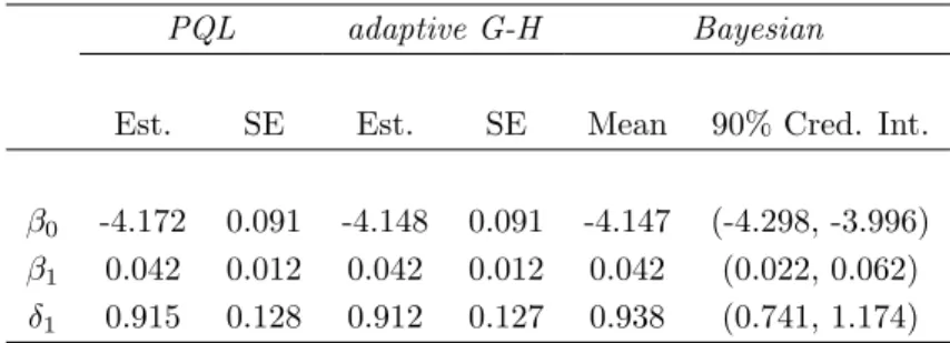
speci-fication in (27) did not lead to convergence of the SAS procedures. Structure (26) is the preferred choice for the linear predictor. Table 5 contains the results of a maximum-likelihood and Bayesian analysis. For the parameterνa uniform prior was specified, other prior specifications were as in Section 3.3.2. Fitted values against real observations are plotted in Figure 9 (right).

For this example the gamma GLMM has an important advantage over the normal mixed model. A linear mixed model is only applicable after a log-transformation of the data (as in the analysis of Frees et al., 2001). However, a correct back-transformation of predictions on the logarithmic scale to the original scale is not straightforward. When using a gamma GLMM this is not an issue, since the data are used in their original form.

Quantiles Gamma (MOM) Loss 0 5*10^6 10^7 1.5*10^7 2*10^7 2.5*10^7 0 5*10^6 10^7 1.5*10^7 2*10^7

Workers’ Compensation Insurance: Losses

Observed Fitted 0 5*10^6 10^7 1.5*10^7 2*10^7 0 5*10^6 10^7 1.5*10^7 2*10^7

Figure 9: Workers’ compensation data (Losses): gamma QQplot of loss.

PQL adaptive G-H Bayesian

Est. SE Est. SE Mean 90% Cred. Int.

β0 -4.172 0.091 -4.148 0.091 -4.147 (-4.298, -3.996)

β1 0.042 0.012 0.042 0.012 0.042 (0.022, 0.062)

δ1 0.915 0.128 0.912 0.127 0.938 (0.741, 1.174)

Table 5: Workers’ compensation data (Losses): results of maximum likelihood and Bayesian analysis. REML is used in PQL.

4.3

Additional comments

GLMMs in Claims Reserving

In Antonio et al. (2006) a mixed model for loss reserving is presented which is based on a data set containing individual claim records. In this way the authors develop an alternative for claims reserving models based on traditional run-off triangles, which are only a summary of an underlying data set containing the individual figures. A general mixed model is then applied to the logarithmic transformed data. Generalized linear mixed models are a valuable alternative, since they do not require a transformation of the data and allow to model the data using (other) distributions from the exponential family.

GLMMs in Credit Risk Modelling

McNeil & Wendin (2005) provide another interesting –financial– application of GLMMs. GLMMs with dynamic random effects are used for the modelling of portfolio credit default

risk. Details on a Bayesian implementation of the models are included.

5

Summary

This paper discusses generalized linear mixed models as a tool to model actuarial longi-tudinal and (other forms of) clustered data. In Section 3 the most important concepts on model formulation, estimation, inference and prediction are summarized. In this way it is our intention to make this literature better accessible to actuarial practitioners and researchers. Both a maximum likelihood and Bayesian approach are presented. Section 4 describes various applications of GLMMs in the domains of credibility, non-life ratemak-ing, credit risk modelling and loss reserving.

A

Maximum likelihood approach: technical details

A.1

(Restricted) Pseudo-Likelihood ((RE)PL)

Consider the response vector Yi (ni ×1) for subject or cluster i (i = 1, . . . , N). Let βˆ

and ˆbi be known estimates of β (p×1) and bi (q×1). Assume that the random effects

have mean0and covariance matrixD, and that the conditional covariance matrix for Yi

is specified as

Var[Yi|bi] =A1µ/i2RiA

1/2

µi . (28)

Hereby Aµi (ni ×ni) is a diagonal matrix with V(µij) (j = 1, . . . , ni) on the diagonal

(see (11)) and Ri (ni ×ni) has a structure to be specified by the analyst (for instance

Ri =φIni×ni). Defineei =Yi−µi and consider a first order Taylor series approximation

of ei about the known estimates ˆβ and ˆbi. We then get

ˆ

ei =Yi−µˆi−∆ˆi(ηi−ηˆi). (29)

Hereby g(µ_i) = η_i = Xiβ+Zibi and ˆ∆i (ni×ni) is a diagonal matrix with the first

order derivative of g−1_{(.) evaluated in the components of ˆη}

i as diagonal elements.

Wolfinger & O’Connell (1993) then approximate the distribution of ˆei givenβ and bi

by a normal distribution with the same first two moments as the conditional distribution of ei|β,bi. Substituting ˆµi for µi in Aµi, this approximation leads to

νi|β,bi ∼ N ³ Xiβ+Zibi,GˆiA1µˆ/i2RiA 1/2 ˆ µi ˆ Gi ´ for νi = g( ˆµi) + ˆGi(Yi−µˆi). (30)

Hereby ˆGi is a diagonal matrix with g

0

( ˆµ_i) on the diagonal. As such, the pseudo data vector νi (which is a Taylor series approximation of g(Yi) around ˆµi) follows a linear

mixed model as specified in (4) with bi ∼ N(0,D) and ²i ∼ N(0,GˆiA1_µˆ/_i2RiA_µ1_ˆ/_i2Gˆi).

Following the approach from linear mixed models, the unknown parameters in D and Ri are estimated by maximizing the log-likelihood (L1) or restricted log-likelihood (L2)

function, with respect to the pseudo-data. Once estimates for the unknown parameters in D and Ri are obtained, the (empirical) maximum likelihood estimator for β and the

Best Linear Unbiased Predictor for bi are obtained with the well-known theory from

linear mixed models. The (restricted) pseudo-likelihood procedure is repeated until the difference between subsequent estimates for ˆD and ˆRi is sufficiently small. As such,

parameter estimates are computed by iteratively applying standard theory from linear mixed models.

A.2

(Adaptive) Gauss-Hermite quadrature

Full details and references on Gauss-Hermite quadrature for mixed models are in Liu & Pierce (1994). Consider first the situation of a single random effect bi. The contribution

of subject i to the marginalized likelihood is given by

Z Yni

j=1

f(yij|bi,β, φ)f(bi|σ)dbi, (31)

where the random effect bi is assumed to follow a normal distribution with zero mean and

standard deviation σ. After a reparameterization to δi =σ−1bi, (31) can be rewritten as

Z Yni

j=1

f(yij|σδi,β, φ)φ(δi; 0,1)dδi (32)

whereφ(δi; 0,1) denotes the standard normal density andf(yij|σδi,β, φ) follows the same

GLM as before but now with g(µij) = x

0

ijβ+zijσδi.

Non-adaptive Gauss-Hermite quadrature approximates an integral of the form

R_+∞

−∞ h(z) exp (−z2)dz by a weighted sum, namely

Z _+∞ −∞ h(z) exp (−z2_{)dz ≈} Q X q=1 wqh(zq). (33)

Q denotes the order of the approximation, the zq are the zeros of theQth order Hermite

polynomial and the wq are corresponding weights. The nodes (or quadrature points) zq

and the weights wq are tabulated in Abramowitz & Stegun (1972, page 924).

The quadrature points used in (33) do not depend onh. As such, it is possible that only very few nodes lie in the region where most of the mass of h is, which would lead to poor approximations. Using an adaptive Gauss-Hermite quadrature rule the nodes are rescaled and shifted such that the integrand is sampled in a suitable range. Assume h(z)φ(z; 0,1)

to be unimodal and consider the numerical integration ofR_−∞+∞h(z)φ(z; 0,1)dz. Let ˆµand ˆ σ be ˆ µ= mode [h(z)φ(z; 0,1)] and σˆ2 ₌ · − ∂ 2 ∂z2ln (h(z)φ(z; 0,1)) ¯ ¯ ¯ z=ˆµ ¸−1 . (34)

Acting as ifh(z)φ(z; 0,1) were a Gaussian density, ˆµand ˆσwould be the mean and variance of this density. The quadrature points in the adaptive procedure, z?

q, are centered at ˆµ

with spread determined by ˆσ, namely

z?

q = ˆµ+

√

2ˆσzq (35)

with (q = 1, . . . , Q). Now rewrite R_−∞+∞h(z)φ(z; 0,1)dz as R_−∞+∞ h(_φz₍)φ_z;(_µ,σz;0₎,1)φ(z;µ, σ)dz, where φ(z;µ, σ) is the Gaussian density function with mean µ and variance σ2_{. Using} simple manipulations it is easy to see that for a suitably regular function v

Z _+∞ −∞ v(z)φ(z;µ, σ)dz = Z _+∞ −∞ v(z)(2πσ2)−1/2exp à −1 2 µ z−µ σ ¶₂! dz = Z _+∞ −∞ v(µ+√2σz) √ π exp ¡ −z2¢_{dz, (36)}

which can be approximated using (33). Applying a similar quadrature formula to

R_+∞

−∞ h(z)φ(z; 0,1)dz and replacing µand σ by ˆµ and ˆσ, we get

Z _+∞ −∞ h(z)φ(z; 0,1)dz ≈√2ˆσ Q X q=1 wqexp (zq2)φ(zq?; 0,1)h(zq?) = Q X q=1 w? qh(zq?), (37)

with the adaptive weights w?

q :=

√

2ˆσwqexp (z2q)φ(z?q; 0,1). (37) is called an adaptive

Gauss-Hermite quadrature formula and can be used to approximate (32).

When bi is a q dimensional vector of random effects, a cartesian product rule based

on (33) (non-adaptive) or (37) (adaptive) can be used to approximate (15), leading to

L(β,α, φ;y) ≈ N Y i=1    Q X i1=1 wi1 Q X i2=1 wi2. . . Q X iq=1 wiq ni Y j=1 f(yij|zi1i2...iq,β, φ)   , (38)

where Q is the order of the numerical quadrature. In this expression the (adaptive) quadrature weightswik (k = 1, . . . , q) and nodeszi1i2...iq (a vector with elements (zi1, . . . , ziq))

depend on the unknown parameters in β, α and φ. Numerical techniques (e.g. Newton-Raphson) lead to ˆα, ˆβ and φ by maximizing (38) over the unknown parameters. Ap-proximate standard errors for β and αare obtained from the inverse Hessian, evaluated at the estimates.

As with general linear mixed models, it is most natural to use Bayesian methods to obtain predictors for the random or subject-specific effects bi (i = 1, . . . , N). Under

linear mixed models the posterior distribution bi|Yi is multivariate normally distributed,

which allows a closed-form expression for the posterior mean. For general linear mixed models this is no longer true and therefore it is customary to use the posterior mode (rather than the mean) to predict bi. When using adaptive Gauss-Hermite quadrature no

extra calculations are required since the mode of f(y_i|bi)f(bi), which equals the mode of

References

[1] Abramowitz, M. & Stegun, I.A. (1972).Handbook of mathematical functions: with formulas, graphs and mathematical tables.Dover, New York.

[2] Antonio, K., Beirlant, J., Hoedemakers, T. & Verlaak, R. (2006). Lognormal mixed models for reported claims reserves.North American Actuarial Journal, 10(1), 1-19.

[3] Booth, J.G. & Hobert, J.P. (1998).Standard errors of prediction in generalized linear mixed models.

Journal of the American Statistical Association, 93(441), 262-272.

[4] B¨uhlmann, H. (1967).Experience rating and credibility I.ASTIN Bulletin, 4, 199-207. [5] B¨uhlmann, H. (1969).Experience rating and credibility II.ASTIN Bulletin, 5, 157-165.

[6] B¨uhlmann, H. & Straub, E. (1970).Glaubw¨urdigkeit f¨ur Schadens¨atze.Mitteilungen der Vereinigung schweizerischer Versicherungsmathematiker, 111-133.

[7] Breslow, N.E. & Clayton, D.G. (1993). Approximate inference in generalized linear mixed models.

Journal of the American Statistical Society, 88(421), 9-25.

[8] Dannenburg, D.R., Kaas, R. & Goovaerts, M.J. (1996).Practical actuarial credibility models. Insti-tute of actuarial science and econometrics, University of Amsterdam, Amsterdam.

[9] Demidenko, E. (2004). Mixed models: Theory and Applications. Wiley Series in Probability and Statistics, Hoboken, New Jersey.

[10] Denuit, M. & Lang, S. (2004).Non-life ratemaking with Bayesian GAMs.Insurance: Mathematics and Economics, 35(3), 627-647.

[11] Diggle, P.J., Heagerty, P., Liang, K.Y. & Zeger, S.L. (2002).Analysis of longitudinal data. Oxford University Press, Oxford.

[12] Fahrmeir, L., Lang, S. & Spies, F. (2003).Generalized geoadditive models for insurance claims data.

Bl¨atter der Deutschen Gesellschaft f¨ur Versicherungsmathematik, 26, 7-23.

[13] Frees, E.W., Young, V.R. and Luo, Y. (1999). A longitudinal data analysis interpretation of credi-bility models.Insurance: Mathematics and Economics, 24(3), 229-247.

[14] Frees, E.W., Young, V.R. and Luo Y. (2001).Case studies using panel data models.North American Actuarial Journal, 5(4), 24-42.

[15] Haberman, S. & Renshaw, A.E. (1996).Generalized linear models and actuarial science.The Statis-tician, 45(4), 407-436.

[16] Hachemeister, C.A. (1975).Credibility for regression models with application to trend.Appeared in:

Credibility, theory and application., Proceedings of the Berkeley Actuarial Research Conference on credibility, Academic Press, New York, 129-163.

[17] Jewell, W.S. (1975). The use of collateral data in credibilty theory: a hierarchical model. Giornale dell’ Instituto Italiano degli Attuari, 38, 1-16.

[18] Kaas, R., Dannenburg, D.R. & Goovaerts, M.J. (1997).Exact credibility for weighted observations.

ASTIN Bulletin, 27(2), 287-295.

[19] Klugman, S. (1992). Bayesian statistics in actuarial science with emphasis on credibility. Kluwer, Boston.

[20] Laird, N.M. & Ware, J.H. (1982). Random-effects models for longitudinal data. Biometrics, 38(4), 963-974.

[21] Liu, Q. & Pierce, D.A. (1994).A note on Gauss-Hermite quadrature. Biometrika, 81(3), 624-629. [22] Makov, U., Smith, A.F.M. & Liu, Y.H. (1996). Bayesian methods in actuarial science.The

Statis-tician, 45(4), 503-515.

[23] McCullagh, P. & Nelder, J.A. (1989). Generalized linear models. Monographs on statistics and applied probability, Chapman and Hall, New York.

[24] McCulloch, C.E. & Searle, S.R. (2001). Generalized, Linear and Mixed Models. Wiley Series in Probability and Statistics, Wiley New York.

[25] McNeil, A.J. & Wendin, J. (2005).Bayesian inference for generalized linear mixed models of portfolio credit risk.Working paper, ETH Z¨urich.

[26] Molenberghs, G. & Verbeke, G. (2005). Models for Discrete Longitudinal Data. Springer Series in Statistics, Springer, New York.

[27] Nelder, J.A. & Verrall, R.J. (1997).Credibility theory and generalized linear models.ASTIN Bulletin, 27(1), 71-82.

[28] Purcaru, O. & Denuit, M. (2003).Dependence in dynamic claim frequency credibility models.Astin Bulletin, 33(1), 23-40.

[29] Scollnik, D.P.M. (1996).An introduction to Markov Chain Monte Carlo methods and their actuarial applications. Proceedings of the Casualty Actuarial Society, LXXXIII, 114-165.

[30] Scollnik, D.P.M. (2000). Actuarial modeling with MCMC and Bugs: additional worked examples.

Actuarial Research Clearing House, 2000.2, 433-585.

[31] Verbeke, G. & Molenberghs, G. (2000).Linear mixed models for longitudinal data. Springer Series in Statistics, Springer, New York.

[32] Wolfinger, R. & O’Connell, M. (1993).Generalized linear mixed models: a pseudo-likelihood approach.

Journal of Statistical Computation and Simulation, 48, 233-243.

[33] Zeger, S.L. & Karim, M.R. (1991).Generalized linear models with random effects; A Gibbs sampling approach.Journal of the American statistical association, 86(413), 79-86.

[34] Zhao, Y., Staudenmayer, J., Coull, B.A. & Wand, M.P. 2005. General design Bayesian generalized linear mixed models. Working paper.